Automatic Construction of Parallel Portfolios via Explicit Instance Grouping

(1)

The Thirty-Third AAAI Conference on Artificial Intelligence (AAAI-19)

Automatic Construction of Parallel Portfolios via Explicit Instance Grouping

∗

Shengcai Liu,

1

_{Ke Tang,}

2†

_{Xin Yao}

2

1_{School of Computer Science and Technology, University of Science and Technology of China, Hefei 230027, China} 2_{University Key Laboratory of Evolving Intelligent Systems of Guangdong Province, Department of}

Computer Science and Engineering, Southern University of Science and Technology, Shenzhen 518055, China [email protected],{tangk3, xiny}@sustc.edu.cn

Abstract

Exploiting parallelism is becoming more and more important in designing efficient solvers for computationally hard prob-lems. However, manually building parallel solvers typically requires considerable domain knowledge and plenty of hu-man effort. As an alternative, automatic construction of paral-lel portfolios (ACPP) aims at automatically building effective parallel portfolios based on a given problem instance set and a given rich configuration space. One promising way to solve the ACPP problem is to explicitly group the instances into dif-ferent subsets and promote a component solver to handle each of them. This paper investigates solving ACPP from this per-spective, and especially studies how to obtain a good instance grouping. The experimental results on two widely studied problem domains, the boolean satisfiability problems (SAT) and the traveling salesman problems (TSP), showed that the parallel portfolios constructed by the proposed method could achieve consistently superior performances to the ones con-structed by the state-of-the-art ACPP methods, and could even rival sophisticated hand-designed parallel solvers.

Introduction

Over the last decade, due to the great development and the wide application of parallel computing architectures (e.g., multi-core CPUs and GPUs) (Asanovic et al. 2009), the available computing power has been dramatically improved. As a consequence, exploiting parallelism is now becoming more and more important in designing efficient solvers for computationally hard problems. Indeed, in some fundamen-tal problem domains such as SAT, the mixed integer lin-ear programming (MILP), and black-box continuous opti-mization, parallel solvers (Biere 2016; Ralphs et al. 2018; Tang et al. 2014) have contributed a lot to the state of the art. However, despite the notable success achieved, the man-ual design of parallel solvers still remains a laborious work.

∗

This work was supported by the National Key Re-search and Development Program of China (Grant No. 2017YFB1003102), the Natural Science Foundation of China (Grant Nos. 61672478 and 61806090), Shenzhen Peacock Plan (Grant No. KQTD2016112514355531), and the Program for University Key Laboratory of Guangdong Province(Grant No. 2017KSYS008).

†

Corresponding author

Typically, this requires almost redesign of existing sequen-tial solvers to involve new mechanisms to handle specific tasks emerged in parallel solving, such as problem decompo-sition, information sharing and cooperative solving, which is non-trivial as identified as the challenge ofstarting from scratchin (Hamadi and Wintersteiger 2013).

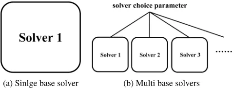
Recently, (Lindauer et al. 2017) studied generic methods for building parallel solvers from existing sequential solvers. The work adopts a simple approach to parallelize a set of se-quential solvers — running them independently in parallel on a given problem instance until the first of them solves it. Such parallel solvers are called parallel portfolios (Gomes and Selman 2001). To determine the solvers in the portfo-lio (called component solvers), a specific problem dubbed automatic construction of parallel portfolios (ACPP) needs to be addressed (Lindauer et al. 2017). More precisely, in ACPP all component solvers are selected from a configura-tion space, with the goal that the performance of the result-ing portfolio on a given problem instance set is optimized. The configuration space is induced by a set of parameterized sequential solvers (called base solvers). As illustrated in Fig-ure 1, if there is only one base solver, the configuration space is exactly the solver’s parameter space; otherwise the config-uration space takes each base solver’s parameter space as a subspace, and would include an additional top-level param-eter to decide which subspace (base solver) would be used. The problem instances in the instance set (called training set) are given by the portfolio user, and should be representative of the target use cases to which the portfolio is expected to be applied. More formally, the ACPP problem could be stated as follow. Given a set of base solvers B and a training set

I, letC denote the configuration space induced byB. The parallel portfolioP withkcomponent solvers is denoted as ak-tuple, i.e.,P = (c1, ..., ck), in whichcirepresents thei

-th component solver ofPand is an individual configuration selected fromC, i.e.,ci ∈ C. The goal of ACPP is to find

c1, ..., ck fromC, such that the performance ofP onI

ac-cording to a given performance metricm(e.g., computation time or solution quality) is optimized.

(2)

con-(a) Sinlge base solver (b) Multi base solvers

Figure 1: Configuration space in ACPP with a single base solver (s1in (a)) and multiple base solvers (s1, s2, ...in (b)).

Each rounded rectangle represents the parameter space of the corresponding base solver.

text of ACPP, the premise for obtaining such a portfolio is thatCcontains complementary configurations. In the litera-ture it has been widely reported (Rice 1976; Xu et al. 2008; Burke et al. 2013; Karafotias, Hoogendoorn, and Eiben 2015) that in many problem domains no single dominant solver exists but different solvers, or different configurations of the same solver, perform best on different problem in-stances. Thus it is suggested that the base solvers used in ACPP should be selected from those sequential solvers that are sufficiently different from each other and meanwhile are highly parameterized with rich configuration spaces. Indeed, as shown in (Lindauer et al. 2017), the performance of the output portfolio would get improved as more diverse solvers are included in the base solver setB.

However, the ACPP problem is far from being satisfac-torily solved. Currently, there are three key ACPP meth-ods, namely GLOBAL, PARHYDRA and CLUSTERING, in which GLOBAL and PARHYDRA are both proposed by (Lindauer et al. 2017) while CLUSTERING is adapted by (Lindauer et al. 2017) from ISAC (Kadioglu et al. 2010) for comparison. These methods adopt different strategies to tackle the ACPP problem. GLOBAL considers it as an algo-rithm configuration (AC) problem by treatingPas a param-eterized solver. By this means the ACPP problem could be directly solved by using the AC procedures existing in the literature. However, the key issue of this method is that its scalability is limited since the size of the configuration space ofP, i.e.,|C|k_{, increases exponentially with the number of}

the component solvers, i.e.,k.

Instead of configuring all component solvers simultane-ously (as GLOBAL does), PARHYDRA configures com-ponent solvers for P one at a time. More specifically, starting from an empty portfolio, PARHYDRA proceeds iteratively and in the i-th iteration it runs an AC pro-cedure to configure ci to add to the current portfolio,

i.e.,(c1, ..., ci−1), such that the performance of the result-ing portfolio, i.e.,(c1, ..., ci−1, ci), is optimized. The main

drawback ofPARHYDRAis that its intrinsic greedy mech-anism may cause stagnation in local optima. To alleviate this problem, a modification was made to PARHYDRA

by allowing simultaneously configuring several component solvers in each iteration. The resulting method is named

PARHYDRAb(Lindauer et al. 2017), whereb(b≥1)

rep-resents the number of the component solvers configured in

each iteration. PARHYDRA and GLOBAL could be both seen as special cases of PARHYDRAb with b = 1and

b = k, respectively. It is conceivable that the choice of b

is very important forPARHYDRAbsince the tendency to stagnate in local optima would increase as b gets smaller, while the size of the configuration space involved in each configuration task inPARHYDRAb, i.e.,|C|b, would grow

exponentially asbgets larger. However, in general the best value ofbmay vary across different scenarios, and for a spe-cific scenario it is very hard to determine a good choice ofb

in advance.

The third method CLUSTERING tackles the ACPP prob-lem via explicit instance grouping. That is, it clusters the problem instances represented in a normalized instance fea-ture space into k subsets and then independently runs an AC procedure on each subset to obtain a component solver. Similar toPARHYDRAb, CLUSTERING also has an im-portant design choice that is hard to determine in advance. Specifically, the clustering result has great influence on the performance of the final parallel portfolio. However, there exists different normalization approaches that can be used here, and different of them can result in different instance clusters. Generally the appropriate choice of the normaliza-tion approach may vary across different instance sets, and the accurate assessment of the cluster quality is not possible before the portfolio is constructed completely.

From a methodological perspective, ACPP methods based on explicit instance grouping seek to achieve the comple-mentarity among the component solvers by promoting each of them to handle different subsets of the problem instances. Thus for these methods the quality of the instance group-ing is crucial. A good instance groupgroup-ing should meet at least one requirement: Instances that are grouped together should be similar in the sense that inCthere exist same good con-figurations for them. Unfortunately, such information is un-known in advance, and thus CLUSTERING uses distances in the feature space to approximate it, which however has been experiementally shown to be ineffective (Lindauer et al. 2017). On the other hand, during the running process of an ACPP method, typically many AC procedure runs would be executed to configure the component solvers. In each AC procedure run many different configurations would be tested on different problem instances; thus a large amount of run-data would be generated, which can be used to help charac-terize the similarity between the problem instances.

(3)

methods, and these portfolios could even achieve the perfor-mance level of parallel solvers designed by human experts.

Related Work

Simultaneously utilizing several complementary solvers is a simple yet effective strategy for solving computationally hard problems. Besides parallel portfolios, this idea has been realized in other forms. Among them the notable ones include sequential portfolios (Rice 1976; Xu et al. 2008; Kotthoff 2014) which try to select the best solvers for ev-ery single problem instance before solving it, and adap-tive solvers such as adapadap-tive parameter control (Karafo-tias, Hoogendoorn, and Eiben 2015), reactive search (Bat-titi, Brunato, and Mascia 2008) and hyper-heuristics (Burke et al. 2013) which seek to dynamically determine the best solver setting while solving a problem instance. In principle, all these methods need to involve some mechanisms (e.g., selection or scheduling) to appropriately allocate computa-tional resource to different solvers, while parallel portfolios do not necessarily require any extra resource allocation since each component solver is simply assigned with the same amount of resource.

ACPP is closely related to the area of automatic algo-rithm configuration, in which the task is to automatically identify a high-quality configuration from a configuration space. In the last few years, several high-performance AC methods (which could handle considerable large configura-tion spaces) such as ParamILS (Hutter et al. 2009), GGA (Ansótegui, Sellmann, and Tierney 2009), irace (López-Ibáñez et al. 2016) and SMAC (Hutter, Hoos, and Leyton-Brown 2011) have been proposed. As a consequence, re-cently there has been research interest in utilizing these AC procedures to automatically identify useful portfolios of configurations from large configuration spaces. Such at-tempts were first done in constructing sequential portfolios. The representative methods for solving this problem are Hy-dra (Xu, Hoos, and Leyton-Brown 2010) and ISAC (Ka-dioglu et al. 2010). The basic ideas of these methods were then adapted to be used in constructing parallel portfolios (i.e., ACPP), thus resulting in PARHYDRA and CLUSTER-ING (Lindauer et al. 2017) (see the first section). The main differences between the automatic construction of sequen-tial portfolios and of parallel portfolios lie in two aspects: 1) The portfolio sizek of parallel portfolios is limited (of-ten by the number of processor cores available), while for sequential portfolios in principle it is unlimited since only some component solvers will be selected to run; 2) Both approaches are bounded by the performance of the portfo-lio’s virtual best solver (VBS). However, parallel portfolios run the whole portfolio in parallel and thus achieve nearly the same performance of the portfolio’s VBS. For sequential portfolios the performance gaps could be larger since the al-gorithm selectors could make mistakes.

Proposed Method

The basic idea of PCIT is simple. Although it is hard to ob-tain a good instance grouping at one stroke, it is possible to gradually improve an instance grouping. PCIT adopts a

random initial grouping; that is, the instances are evenly and randomly divided intoksubsets. The quality of this group-ing could be poor since there is no guidance involved in the grouping procedure. Consider a simple example where in-stance setI={ins1, ins2, ins3, ins4}, configuration space

C = {θ1, θ2}, ins1, ins2 shares the high-quality

config-uration θ1 andins3, ins4 shares the high-quality

configu-ration θ2. Obviously the appropriate grouping for this

ex-ample is {ins1, ins2}{ins3, ins4}, which would lead the

AC procedure to output θ1andθ2on the first and the

sec-ond subset respectively, thus producing the optimal portfo-lioP ={θ1, θ2}. Random grouping strategy may fail on this

example if it happens to splitIas{ins1, ins3}{ins2, ins4}

or{ins1, ins4}{ins2, ins3}, which could cause the AC

pro-cedure to output the same component solver, i.e.,(θ1, θ1)or (θ2, θ2), on both subsets.

The key point here is that if the problem instances grouped together do not share the same high-quality configurations, then the cooperation between the component solvers config-ured on these subsets would be much affected, thus limiting the quality of the final output parallel portfolio. To handle this issue, PCIT employs an instance transfer mechanism to improve the grouping during the construction process by transferring instances between different subsets. More specifically, as the configuration process of a component solver on a subset proceeds, if the AC procedure cannot manage to find a common high-performance configuration for every instance in the subset but only some of them, then it can be inferred that these intractable instances may corre-spond to different high-quality configurations (in the config-uration spaceC) from others. It is therefore better to trans-fer these instances to other subsets that are more suitable to them.

(4)

Algorithm Framework

The pseudo-code of PCIT is given in Algorithm 1. The main difference between PCIT and the existing methods (e.g., GLOBAL and CLUSTERING) is that in PCIT the portfo-lio construction process is divided inton(nis set to 4 in this paper) sequential phases (lines 3-13 in Algorithm 1). The first(n−1)phases serve as adjustment phases, in each of which the instance grouping is adjusted (line 12) once the AC procedures for all component solvers (lines 9-11) finish. The last phase is the construction phase in which the com-ponent solvers of the final portfolio are configured on the obtained subsets with a large amount of time. In fact, the time consumed for the configuration processes in the last phase amounts to the sum of the time consumed for the con-figuration processes in the first(n−1)phases (lines 4-8). One thing which is not detailed in Algorithm 1 for brevity is that, on each subset, to keep the continuity of the config-uration processes across successive phases, the incumbent configuration obtained in the previous phase is always used to initialize the AC procedure in the next phase.

Algorithm 1PCIT

Input:base solversBwith configuration spaceC; number of component solversk; instance setI; performance metric

m; algorithm configuration procedureAC; number of independent runs of portfolio constructionrpc; time budget

for configuration processtc; time budget for validation

processtv; number of stagesn; featuresFfor all instances

inI

Output:parallel portfolio(c1, .., ck) 1: fori:= 1...rpcdo

2: Randomly and evenly splitIintoI1, ..., Ik 3: forphase:= 1...ndo

4: ifphase=nthen

5: t← tc

2

6: else

7: t← tc

2(n−1) 8: end if

9: forj:= 1...kdo

10: Obtain component solvercj by runningAC on

configuration spaceConIjusingmfor timet 11: end for

12: I1, ...Ik ←InsTransfer(I1, ...Ik, c1, ...ck, F) 13: end for

14: Pi←(c1, ..., ck) 15: end for

16: Validate each ofP1, ..., PrpconIusingmfor timetv 17: LetP be the portfolio which achieved the best

valida-tion performance

18: return P

Another important difference between PCIT and the exist-ing methods lies in the way of obtainexist-ing reliable outputs. For existing methods, the uncertainty of the portfolio construc-tion results mainly comes from the randomness of the output of the AC procedure (especially when the base solvers are not deterministic). Thus for each specific algorithm

configu-ration task, typically they conduct multiple independent runs of the AC procedure (with different random seeds), and then validate the configurations produced by these runs to deter-mine the output one. For PCIT, in addition to the randomness mentioned above, a greater source of uncertainty is the ran-domness of the initial instance grouping results. One way to handle both of them is to perform multiple runs of portfolio construction (with different initial instance groupings), and in each construction process the AC procedure is also run for multiple times for each configuration task. In this paper, to keep the design simple, we only allow repeated runs of portfolio construction and rely on the validation to ensure the reliability of the final output (lines 16-18).

Similar to PARHYDRA and CLUSTERING, PCIT con-figures each component solver independently; thus the needed time for construction is linear to the number of com-ponent solvers. Moreover, PCIT can be easily performed in parallel. First, different portfolio construction runs (lines 1-15) can be executed in parallel, and second, during each con-struction run the configuration processes for different com-ponent solvers (lines 9-11) can also be executed in parallel.

Instance Transfer

As shown in Algorithm 2, the instance transfer procedure first builds an empirical performance model (EPM) based on the rundata collected from all the previous AC proce-dure runs (line 1). More specifically, the rundata is actu-ally records of runs of different solver configurations on dif-ferent instances, and each run can be represented by a 3-tuple, i.e.,(conf ig, ins, result). The exact implementation of the EPM here is the same as the one in SMAC (Hutter, Hoos, and Leyton-Brown 2011), which is a random forest that takes as input a solver configurationconf igand a prob-lem instanceins(represented by a feature vector), and pre-dicts performance of conf igonins. The performances of the incumbent configuration on the instances in each subset are obtained by querying the corresponding runs in rundata 1 _{(line 2). After collecting all of them, the median value is}

used to identify the instances that will be transferred (with-out loss of generality, we assume a smaller value is better for

m) (line 3). Then these instances are examined one by one in a random order. Specifically, after an instance is selected to be transferred (lines 7-8), first the built EPM is used to pre-dict the performance of each incumbent on it (lines 9-10); then the target subset of this instance is determined (lines 11-17) according to three rules (line 12): 1) Both the source subset and the target subset will not violate the constraints on the subset size after the instance is transferred; 2) The predicted performance on the instance is not worse on the target subset; 3) The target subset is the one with the best predicted performance among the ones satisfying 1) and 2). The subset size constraints, i.e., the lower boundLand the upper boundU in Algorithm 2, are set to prevent the

occur-1

(5)

rence of too large or too small subsets. In this paperLand

U are set as⌈(1±0.2)|I_k|⌉, respectively. When all the in-stances have been examined, this examination round (lines 6-19) is over. Since the sizes of the subsets keep changing during the instance transfer process, there is a possibility that an instance, which was examined earlier and at that time no target subset satisfying the above conditions was found, has a satisfactory target subset later. To handle this situation, instances which are not successfully transferred in previous rounds will be examined again in the next round (line 20). The whole transfer procedure will be terminated (line 21) if there is no instance that needs to be transferred, or there is no successful transfer occurred in the previous round (lines 6-19). It is thus guaranteed that the transfer procedure will perform at most |T|(i.e., the number of the instances that need to be transferred) examination rounds, in which case in each round a single instance is successfully transferred.

Computational Costs

The computational costs of ACPP methods are mainly com-posed of two parts: the costs of configuration processes and the costs of validation. Specifically, the total CPU time con-sumed isrpc·k·(tc+tv)(the small overhead introduced

by instance transfer in PCIT is ignored here). Similarly, for GLOBAL and CLUSTERING, it israc·k·(tc+tv), where

racis the number of independent runs of the AC procedure

(for each configuration task). ForPARHYDRAb, the

con-sumed CPU time israc·∑ k b

i=1[i·b·(tcb+tbv)], wheretbc

andtb

v refer in particular to the configuration time budget

and the validation time budget used inPARHYDRAb(see (Lindauer et al. 2017) for more details).

Empirical Study

We conducted experiments on two widely studied domains, SAT and TSP. Specifically, we used PCIT to build parallel portfolios based on a training set, and then compared them with the ones constructed by the existing methods, on an unseen test set.

Experimental Setup

Portfolio Size and Performance Metric We set the num-ber of component solvers to 8 (same as (Lindauer et al. 2017)), since 8-core (and 8-thread) machines are widely available now. The optimization goal considered here is to minimize the time required by a solver to solve the problem (for SAT) or to find the optimum of the problem (for TSP). In particular, we set the performance metric to Penalized Aver-age Runtime–10 (PAR-10) (Hutter et al. 2009), which counts each timeout as 10 times the given cutoff time. The optimal solutions for TSP instances were obtained using Concorde (Applegate et al. 2006), an exact TSP solver.

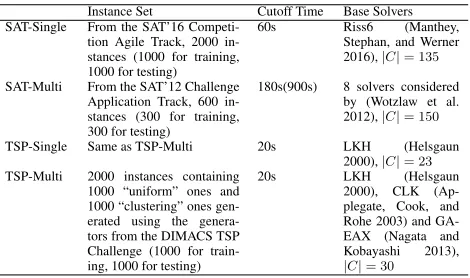
Scenarios For each problem domain we considered con-structing portfolios based on a single base solver and based on multiple base solvers, resulting in four different scenar-ios. For brevity, we use SAT/TSP-Single/Multi to denote these scenarios. Table 1 summarizes the instance sets, the

cutoff time, and the base solvers used in each scenario. Ex-cept in SAT-Multi we reused the settings from (Lindauer et al. 2017), in the other three scenarios we all used new set-tings which had never been considered before in the litera-ture of ACPP. It is especially noted that this was the first time the ACPP methods were applied to TSP. Settings in SAT-Multi are the same as the ones in (Lindauer et al. 2017): 1) Instance set obtained from the application track of the SAT’12 Challenge were randomly and evenly split into a training set and a test set, and to ensure the computational costs for portfolio construction would not be prohibitively large, the cutoff time used in training (180s) was smaller than the one used in testing (900s, same as the SAT’12 chal-lenge); 2) The base solvers in SAT-Multi were the 8 sequen-tial solvers considered by (Wotzlaw et al. 2012) when de-signing pfolioUZK, the gold medal winning solver in the parallel track of the SAT’12 Challenge. The induced config-uration spaceCcontains 150 parameters in total, including a top-level parameter used to select a base solver. In SAT-Single, we chose instances from the benchmark used in the agile track of the SAT’16 Competition for its moderate cut-off time (60s). Specifically, we randomly selected 2000 stances from the original benchmark (containing 5000 in-stances) and divided them evenly for training and testing. We chose Riss6 (Manthey, Stephan, and Werner 2016), the gold medal winning solver of this track, as the base solver. Since Riss6 exposes a large number of parameters, we selected 135 parameters from them to be tunable while leaving others as default. For TSP-Single and TSP-Multi we used the same instance sets. Specifically, we used the portgen and the

portcgengenerators from the 8th DIMACS Implementation Challenge to generate 1000 “uniform” instances (in which the cities are randomly distributed) and 1000 “clustering” instances (in which the cities are distributed around different central points). The problem sizes (the number of the cities) of all these generated instances are within [1500,2500]. Once again, we divided them evenly for training and testing. The base solver used in TSP-Single was LKH version 2.0.7 (Helsgaun 2000) (with 23 parameters), one of the state-of-the-art inexact solver for TSP. In TSP-Multi, in addition to LKH, we included another two powerful TSP solvers, GA-EAX version 1.0 (Nagata and Kobayashi 2013) (with 2 pa-rameters) and CLK (Applegate, Cook, and Rohe 2003) (with 4 parameters), as the base solvers, resulting in a configura-tion space containing 30 parameters (including a top-level parameter used to select a base solver).

Competitors and Time Budgets Besides PCIT, we im-plemented GLOBAL, PARHYDRAb (with b=1,2,4), and CLUSTERING (with normalization options including lin-ear normalization, standard normalization and no normal-ization), as described in (Lindauer et al. 2017)2for compar-ison. For all considered ACPP methods here, SMAC version 2.10.03 (Hutter, Hoos, and Leyton-Brown 2011) was used as the AC procedure. Since the performance of SMAC could be often improved when used with the instance features, we

2

(6)

Table 1: Summary of the instance sets, the cutoff time, the base solvers and the configuration space size in each sce-nario.

Instance Set Cutoff Time Base Solvers SAT-Single From the SAT’16

Competi-tion Agile Track, 2000 in-stances (1000 for training, 1000 for testing)

60s Riss6 (Manthey, Stephan, and Werner 2016),|C|= 135

SAT-Multi From the SAT’12 Challenge Application Track, 600 in-stances (300 for training, 300 for testing)

180s(900s) 8 solvers considered by (Wotzlaw et al. 2012),|C|= 150

TSP-Single Same as TSP-Multi 20s LKH (Helsgaun 2000),|C|= 23

TSP-Multi 2000 instances containing 1000 “uniform” ones and 1000 “clustering” ones gen-erated using the genera-tors from the DIMACS TSP Challenge (1000 for train-ing, 1000 for testing)

20s LKH (Helsgaun 2000), CLK (Ap-plegate, Cook, and Rohe 2003) and GA-EAX (Nagata and Kobayashi 2013), |C|= 30

Table 2: Detailed time budget (in hours) for each method in each scenario. In the experimentsrpc(for PCIT) andrac(for

GLOBAL,PARHYDRAband CLUSTERING) were both set to 10. The 3-tuple in each cell represents (configuration time budget, validation time budget, total CPU time). Given the same configuration budget, the same validation budget andrpc=rac, PCIT, GLOBAL and CLUSTERING would

consume the same amount of CPU time (see the “Computa-tional Costs” part in the last section). Thus M group is used to represent these methods for brevity. ForPARHYDRAb, the configuration budget was set to grow linearly with b, same as (Lindauer et al. 2017).

SAT-Single SAT-Multi TSP-Single TSP-Multi M group (36,4,3200) (80,4,6720) (16,2,1440) (24,2,2080)

PARHYDRA (6,4,3600) (15,4,6840) (3,2,1800) (4,2,2160)

PARHYDRA2 (12,4,3200) (30,4,6800) (6,2,1600) (8,2,2000)

PARHYDRA4 (24,4,3360) (60,4,7680) (12,2,1680) (16,2,2160)

gave SMAC access to the 126 SAT features used in (Hut-ter, Hoos, and Leyton-Brown 2011), and the 114 TSP fea-tures used in (Kotthoff et al. 2015). The same feafea-tures were also used by PCIT (for transferring instances) and CLUS-TERING (for clustering instances). To make the compar-isons fair, the total CPU time consumed by each method was kept almost the same. The detailed setting of the time bud-get for each method is given in Table 2. To validate whether the instance transfer in PCIT is useful, we included another method, named PCRS (parallel configuration with random splitting), in the comparison. PCRS differs from PCIT in that it directly configures the final portfolios on the initial random instance grouping and involves no instance transfer. The time budgets for PCRS were the same as PCIT.

Baselines For each scenario, we identified a sequential solver as the baseline by using SMAC to configure on the training set and the configuration space of the scenario.

Experimental Environment All the experiments were conducted on a cluster of 5 Intel Xeon machines with 60 GB RAM and 6 cores each (2.20 GHz, 15 MB Cache), running Centos 7.5.

Results and Analysis

We tested each obtained solver (including the ACPP port-folios and the baseline sequential solver) by running it on each test instance for 3 times, and reported the median per-formance. The obtained number of timeouts (#TOS), PAR-10 and PAR-1 are presented in Table 3. For CLUSTERING and PARHYDRAb, we always reported the best perfor-mance achieved by their different implementations. To de-termine whether the performance differences between these solvers were significant, we performed a permutation test (with 100000 permutations and significance levelp= 0.05) to the (0/1) timeout scores, the PAR-10 scores and the PAR-1 scores. Overall the portfolios constructed by PCIT achieved the best performances in Table 3. In SAT-Single, SAT-Multi and TSP-Single, it achieved significantly and substantially better performances than all the other solvers. Although in TSP-Multi, the portfolio constructed byPARHYDRAb

obtained slightly better results than the one constructed by PCIT (however the performance difference is insignif-icant), as aforementioned, the appropriate value of b in

PARHYDRAbvaried across different scenarios (as shown in Table 3) and for a specific scenario it was actually un-known in advance (in TSP-Multi it turned out to be 2). Sim-ilarly, as shown in Table 3, the best normalization approach for CLUSTERING also varied across different scenarios. Compared to the portfolios constructed by PCRS, the ones constructed by PCIT consistently obtained much better re-sults, which verified the effectiveness of the instance trans-fer mechanism of PCIT. It is worth noting that GLOBAL performed significantly worse than all the other ACPP meth-ods in TSP-Single and TSP-Multi. This may be because the configuration tasks in GLOBAL (with configuration space size of|C|k_{) are much harder than the ones (with}

(7)

Table 3: Results on the test set in the four scenarios. The name of the ACPP method is used to denote the portfolios constructed by it. The performance of a solver is shown in boldface if it was not significantly different from the best performance (according to a permutation test with 100000 permutations and significance levelp= 0.05). For CLUSTERING andPARHYDRAb, the best performance achieved by their different implementations is reported and the corresponding implementation option, i.e., the choice ofbforPARHYDRAband the normalization approach (“None” for no normalization, “Linear” for linear normalization and “Standard” for standard normalization) for CLUSTERING, is also reported.

SAT-Single SAT-Multi TSP-Single TSP-Multi

#TOS PAR-10 PAR-1 #TOS PAR-10 PAR-1 #TOS PAR-10 PAR-1 #TOS PAR-10 PAR-1

Baseline 383 238 31 71 2275 358 565 118 16 455 99 17

PCRS 234 152 26 44 1435 247 110 31 11 105 30 11

PCIT 181 119 21 35 1164 219 87 24 8 86 24 9

GLOBAL 230 149 25 46 1495 253 224 53 13 150 41 14

PARHYDRAb 235b=4 151 24 40b=1 1326 246 107b=1 29 10 85b=2 24 9 CLUSTERING 227None 146 23 43None 1415 254 121Linear 31 9 99Linear 28 10

ACPP methods here performed much better than the sequen-tial solver baselines, indicating the great benefit by combin-ing complementary configurations obtained from a rich con-figuration space.

Comparison with Hand-designed Parallel Solvers

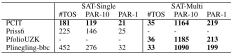
To further evaluate the portfolios constructed by PCIT, we compared them with the state-of-the-art manually designed parallel solvers. Specifically, we considered the ones con-structed for SAT. We chose Priss6 (Manthey, Stephan, and Werner 2016) to compare with the one constructed in SAT-Single, since Priss6 is the official parallel version of Riss6 (the base solver in SAT-Single). For the same reason, we chose PfolioUZK (Wotzlaw et al. 2012) (the gold medal winning solver of the parallel track of the SAT’12 Chal-lenge) to compare with the one constructed in SAT-Multi. Finally, we chose Plingeling (version bbc) (Biere 2016), the gold medal winning solver of the parallel track of the SAT’16 Competition, to compare with both. Note that all the manually designed solvers considered here have imple-mented far more advanced parallel solving strategies (e.g., clause sharing) than only independently running component solvers in parallel. In the experiments the default settings of these solvers were used and the same statistical tests as be-fore were conducted. As shown in Table 4, on SAT-Single test set, the portfolio constructed by PCIT achieved much better results than others. This may be because the parallel solvers considered here were not designed for this type of instances, which were obtained from the SAT’16 Competi-tion Agile track, a track for simple fast SAT solvers with low overhead. On the other hand, this indeed demonstrates that the ACPP methods are widely applicable to different sce-narios, as long as there are suitable base solvers and train-ing instances in the scenarios. It is impressive that, on SAT-Multi test set, the portfolio constructed by PCIT (regardless of its simple solving strategy) obtained slightly better re-sults than pfolioUZK, and could reach the performance level of the more state-of-the-art Plingeling. Such results indicate PCIT could identify powerful parallel portfolios, with little human effort involved. Thus the portfolios constructed by PCIT could conveniently provide at least two advantages. That is, they are high-quality parallel solvers, and they could be used as starting points for the development of more

ad-Table 4: Test results of parallel solvers on the test set of SAT-Single and SAT-Multi. The performance of a solver is shown in boldface if it was not significantly different from the best performance (according to a permutation test with 100000 permutations and significance levelp= 0.05).

SAT-Single SAT-Multi #TOS PAR-10 PAR-1 #TOS PAR-10 PAR-1

PCIT 181 119 21 35 1164 219

Priss6 225 146 25 - -

-PfolioUZK - - - 36 1185 213

Plinegling-bbc 452 276 32 33 1090 199

vanced parallel solvers.

Conclusion

In this paper we proposed a novel ACPP method, named PCIT, which utilized an instance transfer mechanism to im-prove the quality of the instance grouping. The experimen-tal results on two widely studied problem domains, SAT and TSP, have demonstrated the effectiveness of PCIT. Currently PCIT relies on the instance features to build the EPM. Since there are problem domains for which no instance features have yet been defined, it is thus important to investigate how to adapt PCIT to such scenarios. It is also worth investigat-ing the effect of the underlyinvestigat-ing distribution of the instances on the performance of PCIT. Besides, other directions of fu-ture work include extending PCIT to use parallel solvers as base solvers, and investigating solving ACPP from the perspective of subset selection (Qian, Yu, and Zhou 2015; Qian et al. 2017).

References

Ans´otegui, C.; Sellmann, M.; and Tierney, K. 2009. A Gender-Based Genetic Algorithm for the Automatic Configuration of Algorithms. InProceedings of the 15th International Confer-ence on Principles and Practice of Constraint Programming, CP’2009, 142–157.

Applegate, D.; Bixby, R.; Chvatal, V.; and Cook, W. 2006. Con-corde TSP Solver. http://www.math.uwaterloo.ca/tsp/conCon-corde. html.

(8)

Asanovic, K.; Bod´ık, R.; Demmel, J.; Keaveny, T.; Keutzer, K.; Kubiatowicz, J.; Morgan, N.; Patterson, D. A.; Sen, K.; Wawrzynek, J.; Wessel, D.; and Yelick, K. A. 2009. A View of the Parallel Computing Landscape. Communications of the ACM52(10):56–67.

Balyo, T.; Heule, M. J. H.; and J¨arvisalo, M., eds. 2016. Proceed-ings of SAT Competition 2016: Solver and Benchmark Descrip-tions, volume B-2016-1 ofDepartment of Computer Science Se-ries of Publications B. University of Helsinki.

Battiti, R.; Brunato, M.; and Mascia, F., eds. 2008. Reactive Search and Intelligent Optimization. Springer.

Biere, A. 2016. Splatz, Lingeling, Plingeling, Treengeling, Yal-SAT Entering the Yal-SAT Competition 2016. In Balyo et al. (2016), 44–45.

Burke, E. K.; Gendreau, M.; Hyde, M.; Kendall, G.; Ochoa, G.; ¨

Ozcan, E.; and Qu, R. 2013. Hyper-heuristics: A Survey of the State of the Art. Journal of the Operational Research Society 64(12):1695–1724.

Gomes, C. P., and Selman, B. 2001. Algorithm Portfolios. Arti-ficial Intelligence126(1-2):43–62.

Hamadi, Y., and Wintersteiger, C. M. 2013. Seven Challenges in Parallel SAT Solving.AI Magazine34(2):99–106.

Helsgaun, K. 2000. An Effective Implementation of the Lin-Kernighan Traveling Salesman Heuristic. European Journal of Operational Research126(1):106–130.

Hutter, F.; Hoos, H. H.; Leyton-Brown, K.; and St¨utzle, T. 2009. ParamILS: An Automatic Algorithm Configuration Framework. Journal of Artificial Intelligence Research36(1):267–306. Hutter, F.; Xu, L.; Hoos, H. H.; and Leyton-Brown, K. 2014. Algorithm Runtime Prediction: Methods & Evaluation.Artificial Intelligence206:79–111.

Hutter, F.; Hoos, H. H.; and Leyton-Brown, K. 2011. Sequen-tial Model-Based Optimization for General Algorithm Configu-ration. InProceedings of the 5th International Conference on Learning and Intelligent Optimization, LION’2011, 507–523. Kadioglu, S.; Malitsky, Y.; Sellmann, M.; and Tierney, K. 2010. ISAC - instance-specific algorithm configuration. In Proceed-ings of the 19th European Conference on Artificial Intelligence, ECAI’2010, 751–756.

Karafotias, G.; Hoogendoorn, M.; and Eiben, ´A. E. 2015. Param-eter Control in Evolutionary Algorithms: Trends and challenges. IEEE Transactions on Evolutionary Computation 19(2):167– 187.

Kotthoff, L.; Kerschke, P.; Hoos, H.; and Trautmann, H. 2015. Improving the State of the Art in Inexact TSP Solving Using Per-Instance Algorithm Selection. InProceedings of the 9th Inter-national Conference on Learning and Intelligent Optimization, LION’2015, 202–217.

Kotthoff, L. 2014. Algorithm Selection for Combinatorial Search Problems: A Survey.AI Magazine35(3):48–60.

Lindauer, M.; Hoos, H. H.; Leyton-Brown, K.; and Schaub, T. 2017. Automatic Construction of Parallel Portfolios via Algo-rithm Configuration.Artificial Intelligence244:272–290. López-Ibáñez, M.; Dubois-Lacoste, J.; Pérez Cáceres, L.; Stützle, T.; and Birattari, M. 2016. The irace Package: Iter-ated Racing for Automatic Algorithm Configuration.Operations Research Perspectives3:43–58.

Manthey, N.; Stephan, A.; and Werner, E. 2016. Riss 6 Solver and Derivatives. In Balyo et al. (2016), 56.

Nagata, Y., and Kobayashi, S. 2013. A Powerful Genetic Algo-rithm Using Edge Assembly Crossover for the Traveling Sales-man Problem.INFORMS Journal on Computing25(2):346–363. Qian, C.; Shi, J.; Yu, Y.; and Tang, K. 2017. On Subset Selec-tion with General Cost Constraints. InProceedings of the 26th International Joint Conference on Artificial Intelligence, IJCAI’ 2017, 2613–2619.

Qian, C.; Yu, Y.; and Zhou, Z. 2015. Subset Selection by Pareto Optimization. In Proceedings of the 28th Annual Conference on Neural Information Processing Systems, NIPS’2015, 1774– 1782.

Ralphs, T. K.; Shinano, Y.; Berthold, T.; and Koch, T. 2018. Par-allel Solvers for Mixed Integer Linear Optimization. In Hamadi, Y., and Sais, L., eds.,Handbook of Parallel Constraint Reason-ing. Springer. 283–336.

Rice, J. R. 1976. The Algorithm Selection Problem. Advances in Computers15:65–118.

Tang, K.; Peng, F.; Chen, G.; and Yao, X. 2014. Population-based Algorithm Portfolios with Automated Constituent Algo-rithms Selection.Information Sciences279:94–104.

Wotzlaw, A.; van der Grinten, A.; Speckenmeyer, E.; and Porschen, S. 2012. pfolioUZK: Solver Description. In Balint, A.; Belov, A.; Diepold, D.; Gerber, S.; and J¨arvisalo, Matti & Sinz, C., eds.,Proceedings of SAT Challenge 2012 : Solver and Benchmark Descriptions, volume B-2012-2 ofDepartment of Computer Science Series of Publications B, 45. University of Helsinki.

Xu, L.; Hutter, F.; Hoos, H. H.; and Leyton-Brown, K. 2008. SATzilla: Portfolio-based Algorithm Selection for SAT.Journal of Artificial Intelligence Research32:565–606.

(9)

Algorithm 2InsTransfer

Ris the run data collected from all the previous AC proce-dure runs.LandUare the lower bound and the upper bound of the size of a subset, respectively.

Input:instance subsetsI1, ..., Ik, incumbent configurations

c1, ..., ck, instance featuresF

Output:instance subsetsI1, ..., Ik 1: Build anEP M based onRandF

2: For each instanceinsin each subset, obtain the perfor-mance of the corresponding incumbent configuration on it fromR, denoted asP(ins)

3: Letvbe the median value of allP(ins)across all sub-sets. The instances with bigger values thanv are iden-tified as the ones need to be transferred, denoted as T

4: whiletruedo

5: Tdone←∅,Tremain←∅ 6: whileT ̸=∅do

7: Randomly select an instanceinsfromTand letIs

andcsbe the subset containinginsand the

corre-sponding incumbent configuration, respectively

8: T ←T− {ins}

9: For each ofc1, ...ck, useEP M to predict its

per-formance onins, denoted asE(c1), ..., E(ck). 10: Sort c1, ...ck according to the goodness of

E(c1), ..., E(ck), denoted ascπ(1), ..., cπ(k) 11: forj:= 1...kdo

12: ifE(cπ(j))≤E(cs) &&|Iπ(j)|< U&&|Is|>

Lthen

13: Is←Is− {ins}, Iπ(j)←Iπ(j)∪ {ins} 14: Tdone←Tdone∪ {ins}

15: break

16: end if

17: end for

18: ifins /∈TdonethenTremain←Tremain∪ {ins} 19: end while

20: T ←Tremain

21: ifTdone=∅||Tremain=∅then break 22: end while