Forthcoming inErkenntnis. Penultimate version.
Demystifying Dilation
Arthur Paul Pedersen Gregory Wheeler
Abstract
Dilation occurs when an interval probability estimate of some event E
is properly included in the interval probability estimate ofEconditional on every eventFof some partition, which means that one’s initial estimate ofE
becomes less precise no matter how an experiment turns out. Critics main-tain that dilation is a pathological feature of imprecise probability models, while others have thought the problem is with Bayesian updating. How-ever, two points are often overlooked: (i) knowing thatE is stochastically independent ofF (for allF in a partition of the underlying state space) is sufficient to avoid dilation, but (ii) stochastic independence is not the only independence concept at play within imprecise probability models. In this paper we give a simple characterization of dilation formulated in terms of deviation from stochastic independence, propose a measure of dilation, and distinguish between proper and improper dilation. Through this we revisit the most sensational examples of dilation, which play up independence be-tweendilatoranddilatee, and find the sensationalism undermined by either fallacious reasoning with imprecise probabilities or improperly constructed imprecise probability models.
1
Good Grief!
Unlike free advice, which can be a real bore to endure, accepting free information when it is available seems like a Good idea. In fact, it is: I. J. Good (1967) showed that under certain assumptions it pays you, in expectation, to acquire new infor-mation when it is free. This Good result reveals why it is rational, in the sense of maximizing expected utility, to use all freely available evidence when estimating a probability.
Another Good idea, but not merely a Good idea, is that probability estimates may be imprecise (Good 1952, p. 114).1 Sometimes total evidence is insufficient to yield numerically determinate estimates of probability, or precisecredencesas
1Other notable pioneers of imprecise probability include B. O. Koopman (Koopman 1940),
some may say, but instead only yield upper and lower constraints on probability estimates, or indeterminate credal states, as Isaac Levi likes to say (Levi 1974, 1980). The problem is that these two commitments can be set against one another by a phenomenon calleddilation.2 An interval probability estimate for a hypoth-esis is dilated by new evidence when the probability estimate for the hypothhypoth-esis is strictly contained within the interval estimate of the hypothesis given some out-come from an experiment. It is no surprise that new information can lead one to waver. But there is more. Sometimes the interval probability estimate of a hy-pothesis dilatesno matter how the experiment turns out. Here merely running the experiment, whatever the outcome, is enough to degrade your original estimate. Faced with such an experiment, should you refuse a free offer to learn the out-come? Is it rational for you to pay someone tonottell you?
Critics have found dilation beyond the pale but divide over why. For the rear-guard, the prospect of increasing one’s imprecision over a hypothesis no matter how an experiment turns out is tantamount to areductioargument against the the-ory of imprecise probabilities. Conditioning on new information should reduce your ignorance, tradition tells us, unless the information is irrelevant, in which case we should expect there to be no change to your original estimate. However, dilation describes a case where the specific outcome of the experiment is irrelevant but imprecision increases by conditioning, come what may.
The conservatives lament that the proponents of imprecise probabilities trade established distinctions and time-honored methods for confusion and ruin. Simply observing the distinction betweenobjectiveandsubjectiveprobabilities and stick-ing to Laplace’sprinciple of indifference(White 2010), or the distinction between known evidenceandbelief (Williamson 2007, pp. 176-7) and calibrating belief by theprinciple of maximum entropy(Williamson 2010,Wheeler 2012), they argue, would avoid the dilation hullabaloo. The real debate for conservatives concerns which traditions to follow—not whether to abandon numerically determinate prob-abilities. Even some who think that belief states should be indeterminate to “match the character” of the evidence despair of imprecise probability theory ever being of service to epistemology (Sturgeon 2008,2010,Wheeler 2013).
For the vanguard, imprecision is an unavoidable truth, and dilation is but an-other reason to reject Good’s first idea in favor of selective but shrewd updating. Henry Kyburg, for example, long interested in the problem of selecting the appro-priate reference class (Kyburg 1961,Kyburg and Teng 2001), avoids dilation by always selecting the most unambiguously precise estimate available.3 There is no
2The first systematic study of dilation is (Seidenfeld and Wasserman 1993), which includes
histor-ical remarks that identify Levi and Seidenfeld’s reaction to (Good 1967) as the earliest observation of dilation and Good’s reply in (1974) as the first published record. Seidenfeld and Wasserman’s study is further developed in (Herron et al. 1994) and (Herron et al. 1997). See our note 10, below, which discusses a variety of weaker dilation concepts that can be articulated and studied.
3Although evidential probability avoids strict dilation, there are cases where adding new
possibility for dilation to occur within his theory of evidential probability, but this policy is what places evidential probability in conflict with Bayesian conditional-ization (Kyburg 1974,Levi 1977). Even so, the general idea of selective updating may not be incompatible with classical Bayesian methods (Harper 1982). Indeed, one recent proposal to avoid dilation replaces Good’s first principle by a second-order principle purported to determine whether or not it pays you in expectation to update a particular hypothesis on a particular item of evidence (Grünwald and Halpern 2004). This approach faces the problem of how to interpret second-order probabilities (Savage 1972, p. 58), but that is another story.
A point often overlooked by dilation detractors—conservatives and progres-sives alike—is that dilation requires that your evidence about pairs of events in question to not rule out the possibility for some interaction between them (Sei-denfeld and Wasserman 1993). This is a crucial point, for the most sensational alleged cases of dilation—recent examples include (Sturgeon 2010,White 2010, Joyce 2011), but also consider (Seidenfeld 1994)—appear to involve stochasti-cally independent events which nevertheless admit some mysterious interaction to occur. Yet each of these recent examples rests on an equivocation concerning whether the events in question are indeed stochastically independent. If one event is completely stochastically independent of another, an implication of Seidenfeld and Wasserman’s fundamental results on dilation tells us that there is no possibility for one event to mysteriously dilate the other. Claims to the contrary are instances of mishandled imprecise probabilities—not counterexamples to a theory of impre-cise probabilities.
Another source of confusion over indeterminate probabilities is the failure to recognize that there are several distinct concepts of probabilistic independence and that they only become extensionally equivalent within a standard, numerically de-terminate probability model. This means that some sound principles of reasoning about probabilistic independence within determinate probability models are invalid within imprecise probability models. To take an example, within the class of im-precise probability models it does not follow that there must be zero correlation between two variables when the estimate of an event obtaining with respect to one of the variables is unchanged by conditioning on any outcome of the other: one event can beepistemically irrelevantto another without the two events enjoying complete stochastic independence.
The aim of this essay is to help demystify dilation by first giving necessary and sufficient conditions for dilation in terms of deviations from stochastic inde-pendence. Our simple characterization of dilation is new, improving on results of Seidenfeld, Wassermann and Heron, who have provided necessary but insuffi-cient conditions, suffiinsuffi-cient but unnecessary conditions, and characterization results which apply to some classes of models but not to all. We also propose a measure of dilation.
recent line of attack against the theory of imprecise probabilities, and to explain how the theory of imprecise probabilities is more accommodating than some of its advocates have suggested. It should be stressed that this essay offers neither an exhaustive treatment of independence within imprecise probability models,4 nor an exhaustive defense of imprecise probabilities.5 Yet, as should become clear, our characterization results and the role these three independence concepts play are fundamental to understanding imprecise probabilities and their application.
The general class of imprecise probability theories considered in this essay cover several proper extensions of familiar, numerically determinate models: the underlying structure of numerically determinate probability models drop out as a special case of the more general indeterminate theory. This means that the plu-rality of independence concepts, and therefore the underlying mechanics which govern dilation, run deeper than the particular philosophical interpretations which normally lead discussions of theories of probability. As a result, we will make a judicious effort, to the extent we can, to place the mathematics driving dilation in the foreground and the interpretations advanced for different probability models in the background. Proceeding this way is not to devalue questions concerning inter-pretations of probability models. On the contrary, since numerically determinate probability models are simply a special case of this family of imprecise probability models, a large part of the philosophical discussion over proper interpretations can and indeed should be conducted on neutral grounds. This essay may be viewed as a guide to finding that neutral ground.
2
Preliminaries
When you are asked to consider a series of fair coin tosses, what you are being in-vited to think about, in one fashion or another, is an idealized mathematical model: a sequence of independent Bernoulli trials with probability 1/2 for the outcome heads occurring on each toss.
In this section we explain each piece of this mathematical model. In the next we discuss variations of a coin toss experiment consisting of two tosses.
Probability. Aprobability functionis a real-valued functionpdefined on an al-gebraA over a set of statesΩsatisfying the following three conditions:
(P1) p(E) ≥ 0 for everyE∈A; (P2) p(Ω) = 1;
(P3) p(E ∪F) = p(E) + p(F)for all pairwise disjoint elementsEandFinA.
4See (Couso et al. 1999), (Cozman 2012), and (de Cooman and Miranda 2009).
5For instance, Adam Elga’s (2010) alleged counterexample to imprecise decision models
In plain terms, p is a single probability function assigning to each event in the algebraA a numerically determinate real number. The triple(Ω,A,p)is called a
probability space.
For arbitrary eventsE andF inA, an immediate consequence of properties (P1) – (P3) is a generalization of (P3):
(P30) p(E ∪F) = p(E) + p(F) − p(E∩F).
According to one way of understanding imprecision, even thoughpis a single, well-defined function, by strategically withholding information about(Ω,A,p), it
may be only possible to derive an interval constraint for a probability assignment rather than a numerically determinate value.
For example, suppose that numerically precise estimates have been evaluated for a subcollection E ⊆A of events including, say, E andF, but not their joint occurrence,E∩F. In particular, suppose that p(E) =1/2and p(F) =1/2, while a precise value for the binary meet of E and F, E∩F, has not been specified: Solving forβ =p(E∩F)admits any real number within[0,1/2]as a feasible value forβ. This calculation for binary meets and binary joins when only the marginal
probabilities of a pair of events have been specified conforms to the pair of rules from the following proposition.
Proposition2.1 Suppose that p(E)and p(F)are defined. Then: 1. If p(E ∩F) = β, then:
max h
0,p(E) + p(F)
−1
i
≤ β ≤ min
h
p(E), p(F) i
; 2. If p(E ∪ F) = β, then:
max h
p(E), p(F) i
≤ β ≤ min
h
p(E) + p(F),1 i
.
In view of this proposition, a first remark about imprecise probability assign-ments is that they may arise naturally when some information has not been speci-fied. Nothing exotic or heterodox need obscure them.
Affirming a range of solutionsβE for each eventE is to say that there is a set
Pof probability functions assigning real numbersβE to each such eventE. Eachp inPis defined with respect to the same set of statesΩand algebraA. Since the
(P4.1) P(E) = inf{p(E) : p∈P}.
(P5.1) P(E) = sup{p(E): p∈P}.6
If P(F)>0, then conditional lower and conditional upper probabilities are defined, respectively, as follows:
(P4.2) P(E|F) = inf{p(E|F) : p∈P}. (P5.2) P(E|F) = sup{p(E|F) : p∈P}.
Of course, ifF is the sure eventΩ, conditional lower probability and conditional
upper probability reduce to unconditional lower probability and upper probability, respectively.
When lower probability and upper probability agree for all events in the alge-braA, then the setPis a singleton set consisting of a unique precise numerical
probability function onA which realizes the upper and lower probability function: (P6) If P = P, then {p} = P and p = P = P.
Lower probabilities may be defined in terms of upper probabilities, andvice versa, through the following conjugacy relation:
(P7) P(E) = 1 − P(Ec).7
Thus, we may restrict attention to lower probabilities without loss of generality. We remark that lower probabilities aresuperadditive:
(P8) P(E∪F) ≥ P(E) + P(F) − P(E∩F).
By the conjugacy relation (P7), upper probabilities are thereforesubadditive. Given a set of probabilities over an algebraA on a set of statesΩ, let us as before call the
triple(Ω,A,P)aprobability space, and call the quadruple(Ω,A,P,P)satisfying
properties (P4) – (P5) alower probability space.
Finally, we point out that the set of lower probabilities for an eventE,P(E) = {p∈P:p(E) =p(E)}, need not be unique. This is true for the set of upper proba-bilities,P(E) ={p∈P:p(E) =p(E)}, and the corresponding sets of lower
condi-tionals probabilities,P(E|F) ={p∈P:p(E|F) =p(E|F)}, and upper conditional
probabilities,P(E|F) ={p∈P:p(E|F) =p(E|F)}, too.
Think of the conditions for lower probability this way. If we consider a single probability space, Proposition2.1tells us that a gap between lower and upper prob-ability can open only by closing off some part of the algebra from view. Properties (P4) – (P8) accordingly furnish a barebones structure governing sets of probabil-ities to incorporate this game of peekabo directly within the model itself. These properties underlie a proper extension of the standard probability model: there is
6Alternative approaches which induce lower and upper probability are discussed in (Wheeler
2006) and (Haenni et al. 2011).
7Ecis the complement
no reason to deviate from what the fully defined probability function says about events unless some information about the probability space has not been specified. Although it can be useful to imagine the basic model as codifying the conse-quences of unknown parts of the algebra, do not assume that every lower proba-bility model has precise probabilities kept out of sight in a game of peekabo. For example, imagine that a sample of eligible voters is asked whether they intend to vote for Mr. Smith or for his sole opponent in an upcoming election. The lower probability of voting for Smith is the proportion of respondents who pledge to vote for Smith, while the upper probability of voting for Smith is the proportion who have not pledged to vote for his opponent. Rare is the pre-election poll that finds these two groups to be one and the same, for some voters may be undecided, choosing neither to commit to Smith nor to commit to his opponent. The differ-ence between lower probability and upper probability in this case is not due to the pollster’s ignorance of the true strict preferences of the voters but to the presence of truly undecided voters in the sample.
To be sure, if voters must cast a ballot for one of the two candidates, then Smith and his opponent will split the votes on election day, so the proportion of votes cast for Smith will be precisely the proportion of votes not cast for his opponent. But the pre-election poll is designed to estimate voter support for Smith, not to predict the vote count for Smith on election day. The precision of the vote count is irrelevant to resolving the imprecision in a poll of pre-election attitudes. Indeed, often the very point of a pre-election poll is to identify undecided voters as part of an effort to influence how they will cast their ballots on election day.
Stochastic Independence The textbook definition of probabilistic or stochastic independence is formulated in terms of a single probability function. Thus, two eventsEandFinA are said to bestochastically independentjust in case:
(SI) p(E∩F) = p(E)p(F).
In a standard probability space for a precise probability function p, events E and F are stochastically independent just in case conditioning on F is irrelevant to estimating E, and vice versa. Formally, an event F is said to be epistemically irrelevantto an eventEprecisely when:
(ER) p(E|F) = p(E), when p(F) > 0. Accordingly:
(EI) Eis epistemically independent ofF if and only if both Eis epistemically irrelevant toF and Fis epistemically irrelevant toE.
In addition, the degree to which two events diverge from stochastic indepen-dence, if they diverge at all, may be characterized by a simple measure of stochastic independence:
Sp(E,F) =df
p(E∩F) p(E)p(F).
This measure is just the covariance ofEandF,Cov(E,F) =p(E∩F)−p(E)p(F), put in ratio form. Observe that Sp(E,F) =1 just in case E andF are stochas-tically independent; Sp(E,F) > 1 whenE andF are positively correlated; and Sp(E,F) <1 whenE andF are negatively correlated.8 The measureS naturally extends to a set of probability functionsPas follows:
S+P(E,F) =df {p∈P: Sp(E,F) > 1}; S−P(E,F) =df {p∈P: Sp(E,F) < 1}; IP(E,F) =df {p∈P: Sp(E,F) = 1}.
The set of probability functions IP(E,F) fromPwithE andF stochastically
in-dependent is called the surface of independencefor E and F with respect to P.
Subscripts shall be dropped when there is no danger of confusion.
Bernoulli Trials. A Bernoulli trial is an experiment designed to yield one of two possible outcomes,successorfailure, which may be heuristically coded as ‘heads’ or ‘tails,’ respectively. Given a set of statesΩ, the experimentC of interest will
result either in heads or in tails, so either the event (C=heads) obtains or the event(C=tails) obtains. A fair coin toss is a Bernoulli trialCwith probability
1
2 forheads—that is, a Bernoulli trial such that the probability that(C=heads) obtains is 1/2, written p(C=heads) =1/2. In general, a Bernoulli trialC with probabilityθ forsuccessis such that the probability that(C=success)obtains is
θ, p(C=success) =θ.
For a series of coin tosses, letCi be the experimental outcome of theith coin toss. To take an example, consider a sequence of fair tosses for which the probabil-ity that the outcome of the second toss is heads given that the outcome of the first toss is tails, a property which may be expressed as:
p(C2=heads|C1=tails) = 1/2. (1) Notation may be abbreviated by lettingHi denote the event that the outcomeCi is heads on tossi, and by lettingTi refer to the event that the outcomeCi is tails on tossi. With this shorthand notation, Equation (1), for example, becomes:
p(H2|T1) = 1/2.
8The measure S has been given a variety of interpretations in philosophy of science and formal
A sequence of fair coin tosses is a series of stochastically independent Bernoulli trialsC1,...,Cnwith probability 12—that is, a stochastically independent sequence of fair coin tosses C1,...,Cn with p(Ci =heads) = p(Hi) = 1/2 for every i= 1,...,n and p (C1=o1)∩(C2=o2)∩ · · · ∩(Cm =om)
= p(C1=o1)p(C2= o2)· · ·p(Cm=om)for everym≤nsuch thatoi∈ {heads,tails}for eachi=1,...,m. A useful piece of terminology comes from observing that the subset of events
B =
(C=heads),(C=tails)
partitions the outcome spaceΩsince, in the model under consideration, the
out-come of any coin toss must be one element inB. In general, given a probability space(Ω,A,P), call a collection of eventsBfromA apositive measurable
par-tition(ofΩ) just in caseBis a partition ofΩsuch thatP(H)>0 for each partition cellH inB. Note that elements ofBare assumed to be events in the algebraA under consideration unless stated otherwise. In the coin example, the assumption thatBis a positive measurable partition may be reasonable to maintain unless, for example, the coin is same-sided.
3
Dilation
Lower probabilities have been introduced in response to a mischievous riddler who blocks part of the algebra of events from your view in a game of peekaboo, but the question of how to interpret a set of probabilities has been intentionally set in the background. The reason for this is that the barebones model we have presented for a set of probabilities is sufficient to bring into focus the main components needed for dilation to occur, which number fewer than the properties needed to flesh out some natural interpretations for a set of probabilities.
In exchange for leaving the interpretation of a set of probabilities largely un-specified, it is hoped that readers will come to see that dilation does not hinge on whether the set of probabilities in question has been endowed with an interpretation as a model for studying sensitivity and robustness in classical Bayesian statistical inference, or as a model for aggregating a group of opinions, or as a model of indeterminate credal probabilities.
This said, we need to pick an interpretation to run our examples, so from here on we will interpret lower probability as a representation of some epistemic agent’s credal states about events. To make this shift clear in the examples, ‘You’ will denote an arbitrary intentional system, and the set of probabilitiesP in question
will denote that system’s set of credal probabilities. We invite you to play along.9 With these preliminaries in place, we turn now to dilation.
9Alas, ‘You’, you will find, is also a Good idea. This convention has been followed byde Finetti
Dilation. Let(Ω,A,P,P)be a lower probability space, letBbe a positive
mea-surable partition ofΩ, and letE be an event. Say thatBdilates E just in case for
eachH∈B:
P(E|H) < P(E) ≤ P(E) < P(E|H).
In other words,B dilatesE just in case the closed intervalP(E),P(E)is con-tained in the open interval P(E|H),P(E|H)for eachH∈B. The remarkable thing about dilation is the specter of turning amore preciseestimate ofE into a less preciseestimate,no matter what eventfrom the partition occurs.10
Coin Example 1: The Fair Coin. Suppose that a fair coin is tossed twice. The first toss of the coin is a fair toss, but the second toss is performed in such a way that its outcome may depend on the outcome of the first toss. Nothing is known about the direction or degree of the possible dependence. LetH1,T1,H2,T2denote the possible events corresponding to the outcomes of each coin toss.11
You know the coin is fair, so Your estimate of individual tosses is precise. Hence, from P6 it follows that Your upper and lower marginal probabilities are precisely1/2:
(a) P(H1) = P(H1) = 1/2 = P(H2) = P(H2).
It is the interaction between the tosses that is unknown, and in the extreme the first toss may determine the outcome of the second: while the occurrence ofH1 may guaranteeH2, the occurrence ofH1may instead guaranteeT2. Recalling Proposi-tion2.1, suppose Your ignorance is modeled by:
(b) P(H1∩H2) = 0 and P(H1∩H2) = 1/2.
Now suppose that You learn that the outcome of the second toss is heads. From (a) and (b), it follows by (P4) and (P5) that:
10We mention that while our terminology agrees with that ofHerron et al.(1994, p. 252), it differs
from that ofSeidenfeld and Wasserman(1993, p. 1141) andHerron et al.(1997, p. 412), who call dilation in our sensestrict dilation.
Indeed, weaker notions of dilation can be articulated and subject to investigation. Say that a positive measurable partitionBweakly dilates Eif P(E|H) ≤ P(E) ≤ P(E) ≤ P(E|H)for each
H∈B. IfBweakly dilatesE, say that (i) Bpseudo-dilates Eif in addition there isH∈Bsuch that either P(E|H) <P(E) or P(E)< P(E|H)and that (ii) Bnearly dilates Eif in addition for each
H∈B, either P(E|H) < P(E) or P(E) < P(E|H). Thus,Bpseudo-dilatesEjust in case the closed intervalP(E),P(E)is contained in the closed intervalP(E|H),P(E|H)for eachH∈B, with proper inclusion obtaining for some partition cell fromB, whileBnearly dilatesEjust in case the closed intervalP(E),P(E)is properly contained in the closed intervalP(E|H),P(E|H)for eachF∈B.Seidenfeld and Wasserman(1993) andHerron et al.(1994,1997) also investigate near dilation and pseudo-dilation.
11This is Walley’s canonical dilation example (Walley 1991, pp. 298-299), except that here we are
inf
p(H1∩H2) p(H2)
:p∈P
= inf
p(H1∩H2)
1/2 :p∈P
= 2·inf
p(H1∩H2):p∈P
= 0
and
sup
p(H1∩H2) p(H2)
:p∈P
= sup
p(H1∩H2)
1/2 :p∈P
= 2·sup
p(H1∩H2):p∈P
= 1. This yields:
(c) P(H1|H2) = 0 and P(H1|H2) = 1.
So although Your probability estimate forH1 is precise, Your probability estimate forH1given thatH2occurs ismuch lessprecise, with lower probability and upper probability straddling the entire closed interval[0,1]. An analogous argument holds if instead You learn that the outcome of the second toss is tails. SinceB={H2,T2} partitions the outcome space, these two cases exhaust the relevant possible obser-vations, so the probability that the first toss lands heads dilates from 1/2 to the vacuous unit interval upon learning the outcome of the second toss. Your precise probability about the first toss becomes vacuousno matter how the first coin toss
lands.
One way to understand the extremal points P(H1|H2) =0 and P(H1|H2) =1 is as two deterministic but opposing hypotheses about how the second toss is per-formed. One hypothesis asserts that the outcome of the second toss is certain to match the outcome of the first, whereas the second hypothesis asserts that the sec-ond toss is certain to land opposite the outcome of the first. However, after observ-ing the second toss, Your estimate of the first toss becomes maximally imprecise because the two hypotheses predict different outcomes.
4
Dilation Explained
Theorem 4.1 (Seidenfeld and Wasserman, 1993, Theorem 2.2) Let(Ω,A,P,P)
be a lower probability space, letB be a positive measurable partition ofΩ, and
let E∈A. Suppose thatBdilates E. Then for every H∈B:
P(E|H) ⊆ S−P(E,H) and P(E|H) ⊆ S+P(E,H).
Proof. LetH∈B, and suppose that p∈P(E|H).Then:
p(E∩H)
p(H) = P(E|H) < P(E)
≤ P(E)
≤ p(E).
Hence, Sp(E,H)<1, wherebyp∈S−(E,H), establishing thatP(E|H) ⊆S−P(E,H).
An analogous argument for a representativep∈P(E|H)shows that Sp(E,H)>1, establishingP(E|H) ⊆ S+P(E,H).
Theorem 4.2 (Seidenfeld and Wasserman, 1993, Theorem 2.3) Let(Ω,A,P,P)
be a lower probability space, letB be a positive measurable partition ofΩ, and
let E∈A. Suppose that for every H∈B:
P(E)∩S−P(E,H)6=/0 and P(E)∩S+P(E,H)6=/0.
ThenBdilates E.
Proof. LetH∈B, and let p∈P(E)∩S−
P(E,H).Then p(E) =P(E), and since
S−p(E,H)<1, it follows thatp(E∩H)<p(E)p(H), whence: P(E|H) ≤ p(E|H)
= p(E) = P(E).
Therefore, P(E|H) < P(E)for eachH∈B. A similar argument establishes that P(E) < P(E|H)for eachH∈B.
probability function for whichE andH are positively correlated, thenB dilates E.12
We mention that the conclusion of Theorem 4.1is trivially satisfied for each partition cellH for whichP(E|H) orP(E|H) is empty. Similarly, the hypothesis
of Theorem4.2 is vacuously satisfied wheneverP(E)orP(E)is empty. Indeed,
Seidenfeld and Wasserman (1993) frame their results with respect to regularity conditions on the set of probability functionsP, requiring that it be at once aclosed
andconvexset.13 Together, these requirements entail thatP(E|H)andP(E|H)are
nonempty for any eventHwith positive lower probability.
Authors working on imprecise probabilities often require that the set of proba-bilitiesPunder consideration be aclosed convexset. Accordingly, we make some
brief remarks about the elementary mechanics of imprecise probabilities with spect to the important, interdependent roles of closure and convexity. These re-marks are a technical digression of sorts, but they place our later discussion in sharper focus. Readers may wish to skim or skip the next few paragraphs and refer back to them later.
On the one hand, to say that a set of probabilitiesPisclosedis to assert that
the set enjoys a topological property with respect to a topology called the weak*-topologyof the topological dual of a particular collection of real-valued functions equipped with the sup-norm k f k= supω∈Ω|f(ω)|: the set of probabilities in question includes all its limit points, so it is identical to its (topological) closure. Accordingly, in this context, a closed set is calledweak∗-closed. In the finite set-ting, where only finitely many events live in the algebra, a set of probabilitiesP
is weak*-closed just in case it is closed with respect to the total variation norm
kpktv= supA∈A|p(A)|.14
Intuitively, a set of probabilities is closed if the only probability functions “close” to the set are elements of the set: the set of probabilities includes its “end-points,” orboundary. Put differently, any probability function fallingoutside the set of probabilities can be jiggled around a small amount and remain outside the set. To illustrate, consider a probability space for a coin toss for which the set of probabilities includes all probability functions assigning probability greater than 1/4to the event that the coin will land heads. This set of probabilities is not closed because it is missing an endpoint, the probability function assigning1/4to the event that the coin will land heads and3/4to the event that the coin will land tails. By adding this probability function to the set of probabilities, however, the resulting set of probabilities becomes closed.
12Seidenfeld and Wasserman’s results are about dependence of particular events, not about
de-pendence of variables. Indede-pendence of variables implies indede-pendence of all their respective values, but not conversely.
13Specifically,
Pis assumed to be closed with respect to the total variation normSeidenfeld and
Wasserman(1993, p. 1141).
14To maintain brevity, we shall not go into details. See, for example, (Walley 1991, Chapter
On the other hand, to say that a set of probabilitiesPisconvexis to assert that
the set enjoys a vectorial property with respect to pointwise arithmetic operations: the set of probabilities in question is closed under convex combinations—that is, for all p1,p2 ∈P and λ ∈[0,1], λp1+ (1−λ)p2∈P—so it is identical to its
convex hull:
co(P) =df (
n
∑
i=1λipi :λi≥0, pi∈P,and
n
∑
i=1λi=1 )
.
That is, a set of probabilitiesPis convex just in caseP=co(P).
Informally, a set of probabilities is convex if each probability function on a line segment formed from a convex combination of probability functions from the set is also an element of the set. For example, the set of probabilities from the coin toss discussed above is convex since each convex combination of two probability functions from the set of probabilities functions assigning probability greater than 1/4to the event that the coin will lands heads is also an element of the set. However, the set of probabilities consisting of two probability functions—one probability function assigning1/4to the event that the coin will land heads and3/4to the event that the coin will land tails, the second assigning3/4to the event that the coin will land heads and1/4to the event that the coin will land tails—is not convex: A 50-50 convex combination of the two probability functions is not a member of the set of probabilities.
In the finite setting, closure with respect to the total variation norm is equiva-lent to closure with respect to any favored norm of Euclidean space (as they are all equivalent), so a (sequentially) closed set of probabilities is (sequentially) compact. Importantly, when the set of probabilities is in addition convex and lower proba-bility is defined to be the lower envelope P of the setP, as we have done above in
(P4) and (P5), then the lower probability of an event is in fact theminimum num-ber assigned to the event by all probability functions in the set (and not merely the infimum). Indeed, a probability function from the collection ofextreme pointsof the set witnesses the lower probability of the event, and in this setting any compact convex set of probabilities is the convex hull of its extreme points (Walley 1991, pp. 145 ff.).15 Thus, in the finite setting, only some conventional machinery must be employed to get things up and running.
In the general setting, where infinitely many events live in the algebra, some-what fancier machinery must be employed. We discuss the general case in more detail in the Appendix. The upshot is that in both the finite setting and the gen-eral setting, given a nonempty weak*-closed convex set of probabilitiesPand an
eventE, the lower probability ofE, P(E), is given by P(E) =min{p(E):p∈P}.
More generally, when the set of probabilitiesPis no longer required to be
weak*-closed and convex, then where co(P)denotes the weak*-closed convex hull ofP,
we have P(E) =min{p(E):p∈co(P)}. The following proposition records this 15Anextreme pointof a set of probabilities is a probability function from the set that cannot be
property of lower probabilities. We include the proof in the Appendix to illustrate the mechanics discussed above in action.
Proposition 4.3 Let (Ω,A,P,P) be a lower probability space. Then for every
E,H∈A such thatP(H)>0 :
P(E) = minp(E): p ∈co(P) ;
P(E|H) = minp(E|H): p∈ co(P) .
We thus see that specifying P in the quadruple (Ω,A,P,P) does not render Psuperfluous. To be sure, two different sets of probability functions may yield
the same lower probability function. To take a simple example, consider a coin that with lower probability1/4will land heads and with lower probability1/4will land tails. Such a lower probability function may be realized by, for example, the two point setP1=df {p,q}, where passigns probability1/4to heads andqassigns probability1/4 to tails, or by the convex closureP2=df co(P1) =co(P1) (also a weak*-closed set).
Returning to our discussion of dilation, although the conclusion of Theorem4.1 is necessary for dilation, it is easily seen that the conclusion is not sufficient, even if the set of probabilitiesPis weak*-closed and convex, as implied by Proposition
4.3. Assuming that P is weak*-closed and convex, perhaps a second necessary
condition will be enough for sufficiency.
Theorem 4.4 (Seidenfeld and Wasserman, 1993, Theorem 2.1) Let(Ω,A,P,P)
be a lower probability space such thatPis weak*-closed and convex, letBbe a
positive measurable partition ofΩ, and let E∈A. Suppose thatBdilates E. Then
for every H∈B:
P∩IP(E,H) 6= /0.
In other words, a necessary condition for dilation is that the surface of indepen-dence cuts throughP. As Seidenfeld and Wasserman indicate, however, the
condi-tions comprising the conclusions of Theorem4.1and Theorem4.4are again easily seen to be insufficient for the occurrence of dilation.16 Likewise, although the hy-pothesis of Theorem4.2is sufficient for dilation, the hypothesis is not necessary, even ifPis weak*-closed and convex.
Seidenfeld and Wasserman (1993) claim that the aforementioned theorems
show that “the independence surface plays a crucial role in dilation” (p. 1142).
16We note that in their article,Seidenfeld and Wasserman(1993) assume that the set of
Observing that Theorem4.1 and Theorem4.4 offer necessary but jointly insuffi-cient conditions for dilation while Theorem4.2provides a sufficient but unneces-sary condition for dilation, they assert that “a variety of cases exist in between” (Seidenfeld and Wasserman 1993, p. 1142). This remark may leave the impression that the “variety of cases” in between are somehow irreconcilable, resisting a uni-form classification, an impression which may perhaps be supported by Seidenfeld and Wasserman’s hodgepodge of results in a series of articles. While Seidenfeld and Wasserman may have maintained that the “variety of cases” in between resist uniform classification as a result of an analysis tied to viewing dilation through the properties of supporting hyperplanes rather thanneighborhoods, which we intro-duce in the next section, it may very well be that the purpose of pointing to the “variety of cases” in between is simply to frame their research program.
Whatever the case, Seidenfeld and Wasserman (1993), along with Herron (1994, 1997), have explored a number of different cases, sometimes offering necessary and sufficient conditions for dilation with respect to certain regularity assumptions consistent with paradigmatic models.17While focusing on special classes of proba-bility spaces to explore their status with respect to the phenomenon of dilation may be a valuable exercise, the presence of dilation can be straightforwardly shown to admit a complete characterization in terms of rather simple conditions of deviation from stochastic independence. We articulate this characterization in the next sec-tion. Such a characterization may facilitate a smoother, integrated investigation of the existence and extent of dilation as well as questions concerning the preservation of dilation under coarsenings, questions Seidenfeld, Wasserman, and Herron have addressed in their articles. Importantly, investigations and explanations of dilation need not be tied to the particular way in which Seidenfeld and Wasserman have framed their own research program.
5
A Simple Characterization of Dilation
In this section, we offer simple necessary and sufficient conditions for dilation formulated in terms of deviation from stochastic independence, much like the con-ditions from Theorem4.1. We illustrate an immediate application of such a char-acterization with measures of dilation. To begin, we introduce some notation.
Given a nonempty set of probabilities P, eventsE,H ∈ A with P(H) > 0,
andε > 0, define:
P(E|H,ε) =df {p∈P: |p(E|H)−P(E|H)| < ε}; P(E|H,ε) =df {p∈P: |p(E|H)−P(E|H)| < ε}.
We call the sets P(E|H,ε) and P(E|H,ε) lower and upper neighborhoods of E
conditional onH, respectively, with radiusε. Thus, a probability function is an 17They also discuss total variation neighborhoods and
element of a lower neighborhood ofEconditional onHwith radiusε ifp(E|H)is
withinεof P(E|H), and similarly for an upper neighborhood.
Given a nonempty set I, we let RI+ denote the set of elements(ri)i∈I of RI
such thatri>0 for eachi∈I. We now state a proposition characterizing (strict) dilation and then deduce a few immediate corollaries. The proof can be found in the Appendix.
Proposition5.1 Let(Ω,A,P,P)be a lower probability space such thatPis
weak*-closed and convex, letB = {Hi:i∈I}be a positive measurable partition, and let E∈A. Then the following are equivalent:
(i) Bdilates E;
(ii) There is(εi)i∈I∈RI+such that for every i∈I:
P(E|Hi,εi) ⊆ S−(E,Hi) and P(E|Hi,εi) ⊆ S+(E,Hi); (iii) There are(εi)i∈I∈RI+and(εi)i∈I∈RI+such that for every i∈I:
P(E|Hi,εi) ⊆ S
−(
E,Hi) and P(E|Hi,εi) ⊆ S+(E,Hi).
Furthermore, each radius εi may be chosen to be the unique positive minimum of|p(E|Hi)−P(E|Hi)|attained on Ci+=df {p∈P: Sp(E,Hi)≥1}, and similarly each radiusεi may be chosen to be the unique positive minimum of|p(E|Hi)− P(E|Hi)|attained on Ci−=df {p∈P: Sp(E,Hi)≤1}.
Accordingly, Proposition5.1implies that a positive measurable partitionB di-lates an eventE just in case for each partition cellH, there are upper and lower neighborhoods ofE conditional onHsuch that the lower neighborhood ofE con-ditional onH lies entirely within the subset of the set of probabilities in question for whichE andH are negatively correlated, while the upper neighborhood ofE givenH lies entirely within the subset of the set of probabilities in question for whichEandHare positively correlated.
Proposition5.1immediately yields a corollary forarbitrarynonempty sets of probabilities. For the sake for readability in what follows, given a nonempty set of probabilitiesP, letP∗=df co(P)(i.e., the weak*-closed convex hull of P). Thus,
P∗(E|F,ε) =co(P)(E|F,ε) and P∗(E|F,ε) =co(P)(E|F,ε), the written
expres-sions themselves justifying introducing abbreviations. Similarly, let S+∗(E,F)and
S−∗(E,F)be defined by:
S+∗(E,F) =df {p∈co(P):Sp(E,F) > 1} S−∗(E,F) =df {p∈co(P):Sp(E,F) < 1}.
Corollary5.2 Let(Ω,A,P,P)be a lower probability space, let B = {Hi:i∈ I} be a positive measurable partition, and let E∈A. Then the following are equivalent:
(i) Bdilates E;
(ii) There is(εi)i∈I∈RI+such that for every i∈I:
P∗(E|Hi,εi) ⊆ S−∗(E,Hi) and P∗(E|Hi,εi) ⊆ S+∗(E,Hi); (iii) There are(εi)i∈I∈RI+and(εi)i∈I∈RI+such that for every i∈I:
P∗(E|Hi,εi) ⊆ S
−
∗(E,Hi) and P∗(E|Hi,εi) ⊆ S+∗(E,Hi). Furthermore, each radiusεi may be chosen to be the unique positive minimum of
|p(E|F)−P(E|Hi)|attained on Ci+=df {p∈P∗: Sp(E,Hi)≥1}, and similarly for each radiusεi.
The above corollary simplifies in the particularly relevant case in which the positive measurable partitionBis finite.
Corollary 5.3 Let (Ω,A,P,P) be a lower probability space, let B = (Hi)ni=1 be a finite positive measurable partition, and let E∈A. Then the following are equivalent:
(i) Bdilates E;
(ii) There isε>0such that for every i=1,...,n:
P∗(E|Hi,ε) ⊆ S−∗(E,Hi) and P∗(E|Hi,ε) ⊆ S+∗(E,Hi).
Thus, whereas Proposition 5.1 and Corollary 5.2 can ensure a positive real number εi for each i∈I, Corollary 5.3 can ensure a unique positive ε playing the role of eachεi. Like the proof of Corollary5.2, the proof of Corollary5.3 is straightforward, and it may be found in the Appendix.
Proposition5.1and its corollaries should hardly be surprising. The correlation properties that dilation entail are rather straightforward consequences of the defini-tion of diladefini-tion. Moreover, these correladefini-tion properties entail that each dilating par-tition cell and dilated event live on the surface of independence under some prob-ability function from the closed convex hull of the set of probabilities in question. Albeit straightforward results, Proposition5.1and its corollaries show that by look-ingbeyondthe upper and lower supporting hyperplanes P∗(E|H) and P∗(E|H) to
the upper and lower supportingneighborhoods P∗(E|H,ε) and P∗(E|H,ε), it
Seidenfeld, Wasserman, and Herron define a function intended to measure the extent of pseudo-dilation with respect to several statistical models (see footnote 10). Thus, in the present notation and terminology, given a nonempty convex set of probabilitiesP, a finite positive measurable partitionB = (Hi)ni=1and an event E ∈A, Herron et al. (1994, 1997) define what they call the extent of dilation,
∆(E,B), by setting:
∆(E,B) =df min
i=1,...,n
P(E)−P(E|Hi)
+P(E|Hi)−P(E)
.
Seidenfeld, Wasserman, and Herron study how the proposed function measuring the extent to which a finite positive measurable partitionBpseudo-dilatesE may be related to a model-specific index. Of course, for dilation proper, such a function is useful insofar as dilation is known to exist with respect to a model. To be sure, if
∆(E,B)>0, it does not generally follow thatBdilatesE. Although Seidenfeld,
Wasserman, and Herron obtain a number of results reducing∆to model-specific
indices, while sometimes even offering necessary and sufficient conditions for dila-tion stated in terms other than∆, their results in connection with∆cannot generally
be translated to results for dilation proper, as the measure they offer does not re-liably measure the extent ofbona fidedilation. This limitation, however, can be overcome by exploiting the above results.
To illustrate, letPbe a nonempty set of probabilities. Given a positive
measur-able partitionB = {Hi:i∈I}, an eventE∈A, andi∈I, let εE,i and εE,i be real-valued functions defined by setting:
εE,i(p) =df |p(E|Hi) −P(E|Hi)|;
εE,i(p) =df |p(E|Hi) −P(E|Hi)|.
As above, let C−E,i =df {p∈P∗:Sp(E,Hi)≤1} and CE+,i =df {p∈P∗:Sp(E,Hi)≥ 1}.
We may define the ρ∗-maximum dilation, ρ∗, by setting for each eventE∈A
and positive measurable partitionB = {Hi:i∈I}:
ρ∗(E,B) =df η∗(E,B)·ε(E,B)
where:
η∗(E,B) =df sup i∈I
min p∈CE+,i
εE,i(p) + min p∈CE−,i
εE,i(p) !
measures the η∗-maximum extent of dilation, while:
ε(E,B) =df min i∈I maxp∈P∗
1IP(E,Hi)(p)
& min p∈C+E,i
εE,i(p)· min p∈CE−,i
measures the existence of dilation. The pair of brackets d·e denotes the ceiling function. Note the role of the surface of independence in the indicator functions 1I(E,Hi)(where 1I(E,Hi)(p) =1 ifp∈I(E,Hi), and 0 otherwise). In addition, observe
thatρ∗(E,B) = 0 if and only ifBdoes not dilateE, andρ∗(E,B) > 0 if and
only ifε(E,B) =1, so positive values ofρ∗properly report the maximum extent
of dilation. We may say thatPadmits dilationif:
min
(E,B)∈A×Π(P)
ε(E,π) > 0
whereΠ(P)is the collection of all positive measurable partitions ofΩwith respect
toP.
Similarly, we may define the ρ∗-minimum dilation, ρ∗, by setting for each
eventE∈A and positive measurable partitionB = {Hi:i∈I}:
ρ∗(E,B) =df ε(E,B)·max
η∗(E,B),1 +η∗(E,B)
whereεis defined as before and:
η∗(E,B) =df inf i∈I pmin∈C+
E,i
εE,i(p) + min p∈CE−,i
εE,i(p) !
measures the η∗-minimum extent of dilation. Observe that ρ∗(E,B) = 0 if and
only ifBdoes not dilateE, andρ∗(E,B) ≥ 1 if and only ifε(E,B) = 1. The measure∆may also be used. Replacing the ‘min’-operator in the definition ∆with the ‘inf’-operator to ensure generality for partitions of infinite cardinality,
we may define the ∆-minimum dilation, ρ∆, by setting for each eventE∈A and positive measurable partitionB = {Hi:i∈I}:
ρ∆(E,B) =df ε(E,B)·max
∆(E,B),1 + ∆(E,B)
whereε is defined as before. Other measures of dilation may prove to be more useful in some respects, admitting, for example, more or less straightforward re-ductions to model-specific indices.
6
A Plurality of Independence Concepts
the set of probabilities factorize. In other words, within imprecise probability mod-els, even if each event has no effect on the estimate of the other, it still may be that they fail to be stochastically independent events.
The existence of a plurality of independence concepts is a crucial difference between imprecise probability models and precise probability models, for within precise probability models we may reckon that two events are stochastically in-dependent from observing that the probability of one event is unchanged when conditioning on the other. However, this step, from observed irrelevance of one event to the probability estimate of another to concluding that the one event is stochastically independent of the other, is fallacious within imprecise probability models. What this means is that the straightforward path to providing a behavioral justification for judgments of stochastic independence is unavailable when at least one of the outcomes has an imprecise value.18Even so, when the decision modeler knows that one event is irrelevant to another, there are ways to parameterize a set of probabilities to respect this knowledge which, in some cases, suffices to defuse dilation.19
The upshot from these two points is that there are two kinds of dilation phenom-ena, what we callproper dilation andimproper dilation. Theorem4.1, Theorem 4.2, and Theorem4.4, as well as Proposition5.1and its corollaries, hold for both notions. Dilation occurs only if stochastic independence does not hold. However, whereas proper dilation occurs within a model which correctly parameterizes the set of distributions to reflect what is known about how the events are interrelated, if anything is known at all, improper dilation occurs within a model whose pa-rameterization does not correctly represent what is known about how the events interact. If a decision modeler knows that one event is epistemically independent of another, for example, he knows that observing the outcome of one event does not change the estimate in another. That knowledge should constrain how a set of probabilities is parameterized, and that knowledge should override the diluting effects of dilation when updating. Rephrased in imprecise probability parlance, our results and Seidenfeld and Wasserman’s results hold for a variety of natural extensions—including unknown interaction, irrelevant natural extensions, and in-dependent natural extensions (Couso et al. 1999)—but do not discriminate between models which correctly and incorrectly encode knowledge of either epistemic ir-relevance or epistemic independence. Our proposal is that irrelevant natural exten-sions, which correspond to a parameterized set of probabilities satisfying epistemic irrelevance, and independent natural extensions, which correspond to a parameter-ized set of probabilities satisfying epistemic independence, can provide principled grounds for avoiding the loss of precision by dilation that would otherwise come from updating. The upshot is that, even if the conditions for Proposition5.1hold, there are cases where enough is known about the relationship between the events in
18However,Seidenfeld et al.(2010) give an axiomatization of choice functions which can separate
epistemic independence from complete stochastic independence. See (Wheeler 2009b) and (Cozman 2012) for a discussion of these results.
question to support a parameterization that defuses the diluting effect that dilation has upon updating.
An extension in this context is simply a parameterization of a set of probabil-ities, and there are several discussions of the properties of different kinds of ex-tensions (Walley 1991,Cozman 2012,de Cooman et al. 2011,Haenni et al. 2011). Since our focus here is on independence, we will discuss three different classes of parameterizations that correspond to the analogues within imprecise probabilities of our three familiar independence concepts:
(ER) Given P(F),P(Fc)>0, eventF isepistemically irrelevanttoEif and only
if:
1. P(E|F) = P(E|Fc) = P(E); 2. P(E|F) = P(E|Fc) = P(E).
For imprecise probabilities, epistemic irrelevance is not symmetric:Fmay be epis-temically irrelevant toEwithoutEbeing epistemically irrelevant toF.
(EI) Eisepistemically independentofF just when bothF is epistemically
irrel-evant toEandEis epistemically irrelevant toF.
(SI) EandFarecompletely stochastically independentif and only if for allp∈P,
p(E∩F) =p(E)p(F).
We observe that (SI) ⇒ (EI) ⇒ (ER). For suppose that (SI) holds and that
both P(F),P(Fc)>0 and P(E),P(Ec)>0. Then for every p∈P, since p(E∩
F) = p(E)p(F), we have p(E|F) = p(E), so {p(E|F): p∈P}={p(E): p∈ P} and therefore P(E|F) = P(E) and P(E|F) = P(E). Similarly, P(E|Fc) =
P(E), P(E|Fc) =P(E), P(F|E) =P(F), P(F|E) =P(F), P(F|Ec) =P(F), and P(F|Ec) =P(F). Thus, (SI)⇒(EI), and (EI)⇒(ER) follows immediately.
However, (ER)6⇒(EI): although epistemic independence is symmetric, by
definition, epistemic irrelevance is not symmetric. Moreover,(EI)6⇒(SI): two
experiments may be epistemically independent even when their underlying uncer-tainty mechanisms are not stochastically independent. A joint set of distributions may satisfy epistemic independence without being factorizable (Cozman 2012). However, with some mild conditions, whenPis parameterized to satisfy epistemic
independence, some attractive properties hold, including associativity, marginal-ization and external additivity (de Cooman et al. 2011).
7
A Declaration on Independence
by regularity conditions instituted by its Creator, deriving just power from the consent of the epistemic agent—that whenever any governing regularity conditions become destructive of its epistemic ends, it is the right, it is the duty, of the epistemic agent to alter or to abolish them, and to institute new governing conditions, laying its foundation on such principles and organizing its powers in such form, as to them shall seem most likely to effect the agent’s epistemic aims.
Probabilistic independence only appears to be a singular notion when look-ing through the familiar lens of a numerically precise probability function. Thus, constructing an imprecise probability model requires one to make explicit what in-dependence concepts (if any) are invoked in a problem. Example 1, recall, states that the interaction between the tosses is unknown. Compare this example to Ex-ample 2, below, which states that the tosses are independent but does not specify whichnotion of independence is operative.
Coin Example 2: The Mystery Coin. Suppose that there are two coins rather than one.20 Both are tossed normally, but only the first is a fair coin toss. The second coin is a mystery coin of unknown bias.
(d) p(H1) = 1/2 for everyp∈P;
(e) 0 < P(H2) ≤ P(H2) < 1, written p(H2) ∈ (0,1).21
Since both coins are tossed normally, the tosses are performed independently. So, the lower probability of the joint event of heads is approximately zero, and the upper probability of heads is approximately one-half:
(f) P(H1∩H2) = P(H1)P(H2) ≈ 0; P(H1∩H2) = P(H1)P(H2) ≈ 1/2.
Now suppose both coins are tossed and the outcomes are known tousbutnotto You. We then announce to Youeither that the outcomes “match,” C1 = C2,or that they are “split,” C1 6= C2. In effect, either:
(g) We announce that “H1 iff H2” (M), or we announce that “H1 iff T2” (¬M). Since You are told that the first and the second tosses are performed indepen-dently, and initially Your estimate that the outcomes are matched is1/2, then since for eachp∈P:
p(H1) = p(H1|M)p(M) + p(H1| ¬M)p(¬M) = 1/2, (2)
20Variations of this example have been discussed by (Seidenfeld 1994,2007), (Sturgeon 2010),
(White 2010), and (Joyce 2011).
21The open interval (0,1) includes all real numbers in the unit interval except for 0 and 1. This
it follows:
p(H1|M) = 1 − p(H1| ¬M). (3) Also, since for eachp∈P:
p(H2) = p(H2|M)p(M) + p(H2| ¬M)p(¬M) ∈ (0,1), (4) it follows from Equation3:
p(H2) = p(H2|M)p(M) + (1 − p(H1|¬M))p(¬M) = 2p(M)p(H2|M)
Hence, for eachp∈P:
p(H2|M) = p(H2). (5) Equation5implies that our announcing that the two tosses are matched is epistem-ically irrelevant to Your estimate of the second toss landing heads. Analogously, one might also think that announcing that the two tosses are matched is epistemi-cally irrelevant to estimating the first toss. It may seem strange to at once maintain that our announcement is irrelevant to changing Your estimate of a coin that You know nothing about while holding that our announcement is nevertheless relevant to changing Your view about a fairly tossed coin, so one might think
p(H1|M) = p(H1) (6) must hold as well.
However, learning the outcome of the first toss dilates Your estimate that the pair of outcomes match. After all, for all You know, the second coin could be strongly biased heads or strongly biased tails:
P(M|H1) < 1/2 < P(M|H1). Yet sincep(M) =1/2for each p∈P, it follows:
P(M|H1) < P(M) = 1/2 = P(M) < P(M|H1). (7) and a symmetric argument holds if instead the first coin lands tails, so the first coin toss dilates your estimate that toss match.
So, although the second toss is independent of our announcement (Equation5), and the first toss appears to be independent of our announcement (Equation6), our announcing to You that the outcomes match is not independent of the first toss (Equation7) generates a contradiction. So, what gives?
that the first toss lands heads is epistemically relevant to Your estimate of whether the tosses match. Yet Equation 6, if understood to apply to all probability functions from the set of probabilities in question, expresses complete stochastic indepen-dence, which is stronger than mere irrelevance.
In any case, it should be clear that (f) does not entail that our announcement is completely stochastically independent of the first toss. Equation (f) merely says that the coin-tossing mechanism is independent: coins are flipped the same no matter their bias. But suppose thatβis the unknown bias of the second toss landing
heads. Then, condition (f) may be understood to say: p(H1∩H2) = 1/2β
p(H1∩T2) = 1/2(1−β)
p(T1∩H2) = 1/2β
p(T1∩T2) = 1/2(1−β),
which entailsp(H1|M) =β. Therefore, if 0≤β ≤1 is not1/2, our announcement
that the outcomes match cannot be stochastically independent of Your estimate for the first coin landing heads.
This observation is what is behind Jim Joyce’s (2011) response to Example 2, which is to rejectp(H1|M) =p(H1)in Equation6.
There are two ways in which one event can be “uninformative about” an-other: the two might be stochastically independent or it might be in an “un-known interaction” situation. RegardingM andH1as independent in Coin Game means having a credal state p(H1|M) =p(H1) =p(M) =1/2holds everywhere. While proponents of [The principle of Indifference] will find this congenial, friends of indeterminate probabilities will rightly protest that there is no justification for treating the events as independent (Joyce 2011,
our notation).
According to bothJoyce(2011) andSeidenfeld(1994,2007), announcing “match” or “split” dilates your estimate of the first toss from1/2, and itshoulddilate Your estimate because either announcement is “highly evidentially relevant toH1even when you are entirely ignorant ofH2” (Joyce 2011).
Yet suppose you start with the idea that Your known chances about the first toss should not be modified by an epistemically irrelevant announcement. After all, how can You learn anything about the first toss by learning that it matches the outcome of a second toss about which You know nothing at all? Yet this commit-ment combined with (f) appears to restrictβ to1/2and rule out giving the second toss an imprecise estimate altogether. This observation is what drives Roger White (2010) to view the conflict in Example 2 to be a decisive counterexample to impre-cise credal probabilities.
◦ Idem quod Joyce, pace White:
The first toss and the announcement “match” are dependent; however,
◦ Idem quod White, pace Joyce:
The announcement “match” is irrelevant to Your estimate of the first toss. Indeed, in presenting our blended set of conditions for the mystery coin exam-ple, we are less interested in defending our proposal asthecorrect model for the mystery coin than we are in demonstrating that imprecise probability models are flexible enough to consistently encode seemingly clashing intuitions underpinning the example. Put differently, both Joyce and White make a category mistake in staking out their positions on the mystery coin case. The argument is over model fitting—not the coherence of imprecise probability models.
White commits a fallacy in reasoning by falsely concluding that epistemic irrel-evance is symmetric within imprecise probability models, and by falsely supposing one event as epistemically irrelevant to another only if the two are stochastically in-dependent. Joyce, failing to distinguishproperfromimproperdilation, concludes, invalidly, that he is compelled by the internal logic of imprecise probability models to maintain that the announcement dilates Your estimate of the first toss.
Blocking Dilation Through Proper Parameterization. Let us explore how to consistently represent the two claims that set Joyce and White apart in Example 2. Start with the observation that the pair of coin tosses yields four possible out-comes. A joint probability distribution may be defined in terms of those four states, namely:
p(H1∩H2) =α1 p(T1∩T2) =α4 p(H1∩T2) =α2 p(T1∩H2) =α3.
Given this parameterization, a setP of all probability measures compatible with
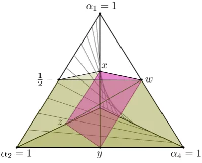
what we know about the tosses can be represented by a unit tetrahedron (3-simplex), Figure1illustrates this parameterization, where maximal probabilities for each of the four possible outcomes corresponds to the four vertices,
α1=1 (1,0,0,0),
α2=1 (0,1,0,0),
α3=1 (0,0,1,0),
α4=1 (0,0,0,1).
setPof measures, the entire tetrahedron would represent the admissible values.22
So, what You know initially about the coin tosses will translate to conditions that constrain the space of admissible probabilities, which we can visualize geometri-cally as regions within the unit tetrahedron, and what You learn by updating will translate to some other region within this tetrahedron. Different independence con-cepts translate to different ways of rendering one event irrelevant to another, but not every way of interpreting independence is consistent with the information provided by Example 2.
Now consider how the key constraints in Example 2 are represented in Figure1. (d) Within the unit tetrahedron there are four edges on which the constraint1/2 on outcomeH1appears: the pointsxon the edgeα1α3,yon the edgeα2α4, zon the edgeα2α3, andwon the edgeα1α4. The omitted two edges specify
either thatH1 is certain to occur or thatT1 is certain to occur, respectively. So, the hyperplanexwyzrepresents the constraintp(H1) =1/2.
(e) The entire tetrahedron represents p(H2)∈[0,1].
(f) i. The upper and lower probabilities of both tosses landing heads is picted by the shaded pentahedron, where the base of this polytope de-fined by the coordinates α2, α3, α4 represents the lower probability P(H1∩H2) =0, and the top of the polytope defined by x,wand the corresponding sharp value1/2marked on theα1α2edge represents the upper probability P(H1∩H2) =1/2.
ii. TossC1 is independent of C2,23 so I(C1,C2)6= /0 but S+(C1,C2) =
S−(C1,C2) = /0. At minimum, the outcome of the first toss is epistem-ically independent of the outcome of the second. This independence condition is represented by the saddle-shaped surface of independence connecting the orthogonal axesα1α2 andα2α4in Figure1, represent-ing thep∈Psuch that
p(H2|H1) =p(H2) =p(H2|T1). (8) Symmetrically, this is precisely the p∈Pthat connect the orthogonal axesα1α3andα2α4and satisfy
p(H1|H2) =p(H1) =p(H1|T2). (9) Equation8 says that the outcome of the first toss is epistemically ir-relevant to Your estimate of heads occurring on the second toss, and Equation9 says that the outcome of the second toss is epistemically irrelevant to Your estimate of heads occurring on the first toss. Taken together we have that the first toss is epistemically independent of the second toss.
22If
Pis closed and convex, then every point in the tetrahedron is admissible if the constraint is
the closed unit interval[0,1].
23Recall that the random variablesC
iii. The only region satisfying independence (ii), the interval constraint on the joint outcome of heads on both tosses (i), the sharp constraint on the first toss landing heads (d), and the interval constraint on the second toss landing heads (e), is the line segmentxy, which rests on the surface of independence determined by Equations8and9.
(g) Suppose that we announce that the outcomes match,C1=C2.Mis the edge
α1α4. Suppose instead that we announce that the outcomes split,C16=C2.
¬Mis the edgeα2α3.
α1 = 1
α2= 1 α4= 1
1
2 – w
z
x
y
Figure 1: The constraints on Coin Example 2.
On this parameterization, the pair of coin tosses are epistemically independent and this relationship is represented by the saddle-shaped surface of independence satis-fying Equations8and9. Furthermore, Your initial estimate that we will announce “match” is1/2, which is the point at the dead center of the polytope: the intersection of the lineszwandxy. This point also sits on the surface of independence.
However, the announcement “match” is the edgeα1α4, which is entirely off of the surface of independence for the two coin tosses. The same is true if instead we announce “split”, which is the edgeα2α3. So, announcing whether the two tosses
are the same or they differ is not independent of the outcome of the first toss. Here we are in agreement with the first half of Joyce’s analysis.
The question now is whether this failure of independence between announcing “match” and the first toss is sufficient to ensure that this announcement is epistem-ically relevant to You. There is a sense in which learning whether the outcomes match or split is epistemically irrelevant to Your estimate of heads. This raises two questions. First, is there room within an imprecise probability model to accommo-date this view? Second, if so, is it a rational view to maintain? Let’s address the first question here and return to the second in the next section.
distribu-tionsP1andP2is the the setPof all joint distributionspwhich have the form
p(H1∩M) =p1(M)p2(H1|M),
for some p1 ∈P1 and p2(· | M) ∈P2. Here the point w in Figure 1 denotes
p2(H1|M) =1/2. Thus, the joint set of distributions constructed by anyp1(M)∈P1 will do, since all are1/2, but the setP2is restricted to p2(H1|M) =1/2. With these selections for the marginal set of distributions P1 and P2 and the judgment that announcing “match” is epistemically irrelevant to Your probability estimate of the first coin landing heads, the set of joint distributionsP(H1∩M)encodes that learn-ing M is an irrelevant extension of Your estimate of 1/2 that the first toss lands heads. Thus, we may agree with Joyce that the first toss and our announcement are probabilistically dependent but still maintain Equation6 on the grounds that the announcement is irrelevant to the first toss. Likewise, a dual argument holds for pointzwherep2(H1| ¬M) =1/2.
However, learning that the first toss is heads is epistemically relevant to Your estimate of whether we will announce “match” or announce “split.” After the first coin is tossed, Your estimate of Mdilates from 1/2to (0,1)because You remain completely ignorant of the bias of the second coin. This means that our method for constructing the set of joint distributions,P(M∩H1), cannot be the same method we used above to construct the irrelevant natural extension ofP1(H1)andP2(H1| M). Here the pointsw,x,y,zin Figure1represent p1(H1) =1/2, but conditioning reduces to the line segmentzw, sincep(M|H1)∈(0,1)6=p(M).
For this example we have an imprecise probability model which accommo-dates the fact that our announcement is not independent of the first toss. Indeed, on this model the two are neither stochastically independent nor epistemically inde-pendent. Even so, there is room to accommodate the view that our announcement is irrelevant information to Your estimate about whether the first coin toss lands heads. Moreover, due to the asymmetry of epistemic irrelevance, You can maintain that the announcement is irrelevant to the first toss even though the first toss dilates Your estimate about the announcement!
Accommodating the conflicting intuitions about Example 2 involves exploit-ing the distinction between epistemic independence, which is symmetric, and epis-temic irrelevance, which is not. Even so, there is also a difference between stochas-tic independence and epistemic independence. Equations8and9together express that the coin tosses are epistemically independent, but they do not specify that the tosses are completely stochastically independent. To get at the difference between these two independence concepts, consider another example which illustrates a set of distributions that satisfies epistemic independence but fails to satisfy complete stochastic independence.