The effect of temperature‑dependent
thermal conductivity on the geothermal
structure of the Sydney Basin
Alexandre Lemenager
*, Craig O’Neill
*, Siqi Zhang and Morgan Evans
Background
In this study, thermal temperature-dependent conductivity measurements are used to generate thermal models. This is done to constrain the temperature distribution in the Sydney Basin down to a depth of 12 km. Understanding the thermal struc-ture of sedimentary basins has worldwide applications, and in this study the Sydney Basin is used as a proxy. Urban and rural areas could greatly benefit from an alter-native energy source such as geothermal energy, tapping into heat trapped beneath coal seams and insulating sediments. The depth of investigation potentially probes down from 1.5 to 4 km; desirable drilling depths would in turn depend on the use of the geothermal location, whether it be used for heating or producing electric-ity. Naturally, the shallower the depth, the more economical the exploration pro-cess becomes. This depth range generally implicates hot-dry rock systems (HDR),
Abstract
The thermal structure of continental crust is a critical factor for geothermal exploration, hydrocarbon maturation and crustal strength, and yet our understanding of it is limited by our incomplete knowledge of its geological structure and thermal properties such as hydrogeologic and thermo-mechanical feedbacks that come into play. One of the most critical parameters in modelling upper crustal temperature is thermal conductiv-ity, which itself exhibits strong temperature dependence. In this study, we integrate new laboratory measurements of the thermal conductivity of Sydney Basin rocks under varying temperatures, with finite-element geothermal models of the Sydney Basin using deal.II (Bangerth et al. in ACM Trans Math Softw (TOMS) 33:24, 2007). Basin geometry and structure are adapted from Danis et al. (Aust J Earth Sci 58:517–42, 2011), which quantified the extent of Triassic sediment, Permian coal measures, Carboniferous volcanics and thickness of the crystalline crust. We find that temperature-dependent thermal conductivity results in lower lateral variations in temperature compared to constant thermal conductivity models. However, the average temperatures at depth are significantly higher when temperature-dependent thermal conductivity effects are included. A number of regions within the Sydney Basin demonstrate temperatures above 150 °C at depths of less than 2000 m in these models, for instance NW of Single-ton, exhibits a strong thermal anomaly, demonstrating the potential for geothermal prospectivity of the region from experimentally constrained thermal parameters.
Open Access
© The Author(s) 2018. This article is distributed under the terms of the Creative Commons Attribution 4.0 International License (http://creat iveco mmons .org/licen ses/by/4.0/), which permits unrestricted use, distribution, and reproduction in any medium, provided you give appropriate credit to the original author(s) and the source, provide a link to the Creative Commons license, and indicate if changes were made.
RESEARCH
*Correspondence: [email protected]; alexandre.lemenager@students. mq.edu.au; craig.
rather than porous thermal fields that usually occur at shallower depths. HDR sys-tems typically require more research and reliable models to ensure safer investments and drilling successful targets. The large-scale impact of aquifers on heat flow in the Sydney Basin is not entirely understood; however, its effect can be considered neg-ligible assuming groundwater systems only have a significant impact within the top 100 m (Danis et al. 2012), as observed by the Sydney Catchment Authority through groundwater monitoring boreholes located in the Ulan Coal Mines, concluding that seasonal variations are no longer detected below 100 m.
Variables used to set up the model have been adapted from Danis et al. (2012), who have produced thermal models of the Sydney Basin, based on constant ther-mal conductivity values. These therther-mal models were constrained using equilibrated borehole temperature measurements from shallow groundwater in the Sydney Basin. However, large-scale effects of temperature-dependent thermal conductivity have yet to be implemented in current models regarding the Sydney Basin.
This study aims to assess how much of an effect variable thermal conductivity has on the large-scale temperature distribution of the Sydney Basin, particularly when compared against constant thermal conductivity models.
To do this, finite-element simulations were performed which result in a model of the temperature distributions of the Sydney Basin at depth, incorporating the effects of the basin stratigraphy, heat-producing values and variations in thermal conductivity.
The thermal conductivity of Sydney Basin sediments (incorporating sandstone and coal) and basement (consisting of Lachlan Fold Belt granitoids) have a significant tem-perature dependence based on the measurements in this study. It is currently thought that the addition of temperature-dependent thermal conductivity data in geothermal simulations will result in significantly different temperature distributions at depth.
At temperatures lower than 700 °C, assuming a constant pressure, the main energy transfer mechanism is thermal conduction within a porous medium such as sand-stone (Abdulagatova et al. 2009). Therefore, a gradual shift in temperature causing a subsequent change in thermal conductivity is thought to have rather significant impacts on the overall thermal structure of our models as temperatures converge to 350 °C at the bottom boundaries. The role of thermal diffusivity in the propagation of thermal energy is similarly relevant in the scope of cooling rates in granitic plutons and basaltic sills (Nabelek et al. 2012).
Geological background
The Sydney Basin can be described by a two-phase stratigraphic model for foreland-basin development. The Sydney Basin formation process consisted of a foreland-foreland-basin deposition component—a result of tectonic loading (the syn-orogenic phase), and a basin response to thrust-belt erosion (post-orogenic phase) (Heller et al. 1988).
The Sydney Basin is located between the New England and Lachlan Fold belts and consists of Permian–Triassic sedimentary sequence of at least 4 km thick (Middleton and Schmidt 1982). At its thickest point, the Sydney Basin is cross-cut by the north-easterly dipping frontal thrust fault of the Tamworth Arc of the New England Fold belt, and gradually thins towards the south (Conaghan et al. 1982). This trend is evident in the compiled gravity profiles sourced from Danis et al. (2011) used to define basin geometry at a relatively high spatial resolution. The Sydney Basin is essentially a succession of Per-mian to Triassic sedimentary and scattered volcanic rocks formed as a result of basin extension, outcropping in a NW to SE trend.
Fore-arc basin sedimentation and orogenic recession via crustal thinning has resulted in thermal subsidence, accumulating large coal reserves—among some of the largest in the world (Casareo 1996). These large coal reserves mostly consist of the Northern Sydney Basin Permian Coal Measures. Local bioturbations have been found to protrude the Newcastle coal measures, while the Newcastle coal measures have a predominantly dominant fluvial signature, containing plant fragments and upward fining sandstone and overbank sediments such as claystone (Hunt et al. 1984). The Newcastle coal measures appear as lenses within a large suite of terrigenous sediment (Herbert 1995). Therefore for the purposes of this work, the Newcastle and Tomago coal measures are grouped as one major coal layer with their terrigenous components reflected in their bulk thermal conductivity. The Waratah sandstone sequence denotes a period of extended transgres-sion and has signs of re-working indicating evidence of basin-wide shoreline re-working shown by angular disconformities at the contact between the Tomago and Newcastle coal measures (Conaghan et al. 1982). The Waratah sandstone marks a geological point separating organic-rich coal sequences and the largely terrigenous Triassic sediments.
Previous thermal modelling
Thermal modelling of the Sydney Basin has recently been undertaken by Danis et al. (2012), as part of the large-scale study of the Sydney–Bowen–Gunnedah Basin (Danis and O’Neill 2010). Thermal models of Danis et al. (2012) were developed using a finite-element code, named “Underworld” designed by Moresi et al. (2007). The model applies constant top and bottom conditions of 15 and 350 °C, respectively, with reflecting side conditions. The top temperature of 15 °C was adopted from Cull’s (1979) yearly average surface temperature measurements of the Gunnedah Basin. The bottom temperature of 350 °C was constrained through extrapolation of groundwater borehole temperature measurements, taken across the Sydney Basin, and this boundary condition was modi-fied to optimise the fit between the steady-state models, and observed geotherms.
temperature accommodate for larger uncertainties across modelled geotherms (Danis et al. 2012) within the shallow crust, such that extrapolated temperatures based on groundwater borehole temperature measurements have a margin of error substantially higher than the extrapolated temperature of deep crust (down to 12 km in this case), mostly due to the absence of groundwater and seasonal effects at such depths (> 100 m).
Numerical models by Danis et al. (2012) incorporate the effects of basin architecture and geology with measured and extrapolated temperature conditions in order to provide a more realistic representation of the distribution of temperature of the Sydney Basin. It was pointed out by Danis et al. (2012) that the refraction of heat around insulating coal layers would likely have a significant impact on local geotherms with coal seams in their direct vicinity. As a result, the impact of coal in thermal models warrants further exami-nation. The thermal models of Danis et al. (2012) also take into account the topography of thermal profiles, through ground surface elevation measurements. Topographic sur-face variations result in localised additions or deficiencies of sedimentary cover, which can have a substantial effect on subsurface temperatures, and shallow heat flow direc-tions (Danis et al. 2012).
Methods
Thermal conductivity measurements
Thermal conduction is thought to be the dominant heat propagation mechanism in sedimentary basins, alongside advection of heat through groundwater motion (Clauser and Huenges 1995). Conduction itself is dependent on the composition of the medium (thermal conductivity), its temperature (in the case of temperature-dependent thermal conductivity) and the temperature gradient across a system. Temperature has a more dominating effect than pressure in crustal settings (Vosteen and Schellschmidt 2003), and therefore temperature alone will in parallel with thermal conductivity and heat gen-erating will be accounted for in our models. In addition, thermal conductivity and tem-perature gradient negatively correlate, where an increase in thermal conductivity results in a reduction in temperature gradient, highlighting that heat flow is highly dependent on thermal conductivity (Sass et al. 1992).
The thermal conductivity of a specimen may be measured in situ or in the laboratory. In situ measurements accounts for a larger volume or rock, while it is easier to control temperature, pressure and pore-fluid variables with laboratory measurements (Clauser and Huenges 1995).
In addition to a rock’s isotropy or anisotropy, thermal conductivity is a function of temperature (Clauser and Huenges 1995). Generally, thermal conductivity reduces with temperature, as differential expansion can lead to contact resistances between grains boundaries.
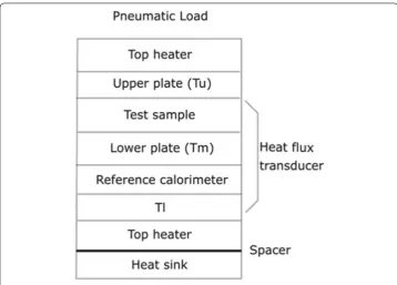
At thermal equilibrium, the Fourier heat flow equation applied to the test stack becomes (Anter Manual 2011)
where Rs is thermal resistance of the sample, F is the heat flow transducer calibration factor, Tu is the upper plate surface temperature, Tl is the lower plate surface tempera-ture, Q is the heat flow transducer output and Rint is the interface thermal resistance. The sample thermal conductivity, λ, is calculated by dividing sample thickness by its measured thermal resistance from the previous equation.
The pneumatic load is set at a constant 20 MPa throughout thermal conductivity measurements.
Internal precision values and calibration
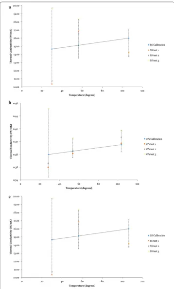
A set of calorimeters were used in the thermal conductivity measurement process of sandstone, coal and granite in the laboratory. The most recent calibration done on the samples measured is shown in the form of a calibration curve in Fig. 3a, b.
Calibration specimens (Additional file 1: Table S1) were repeatedly measured to con-strain instrument internal precision values. Each calibration specimen was measured a total of three times, excluding the initial calibration process. These measurements were compared to initial calibration values, and their deviation from original measurements
Rs=F·Tu −Tl
Q −Rint,
= d
Rs
was recorded. Internal precision measurements were only done for low-temperature set points, as the uncertainty in thermal conductivity is highest at low temperatures. The following plots show thermal conductivity variation of calibration specimens with repeated measurements.
As the internal precision measurement plots suggest, uncertainty between measure-ments reduces greatly with temperature, and the uncertainty associated with the 100 °C temperature set point can be used for high-temperature measurements.
Thermal conductivity tests of samples were done at pre-determined temperature intervals of 20°, 50° and 100° for low-temperature tests; and 100°, 150°, 200°, 250° and 300° for high-temperature tests. Low- and high-temperature tests are performed sepa-rately, as they each require different spacers manufactured from copper and polymide, respectively. Each spacer is selected for its affinity to retain a relatively stable thermal conductivity within a low- and high-temperature range.
Minimum standard deviations were assigned to each specimen, which were calculated based on the repeated thermal conductivity measurement of calibration specimens. Standard deviation values were derived from one calibration only, the same calibration used for the coal thermal conductivity measurements. Low- and high-temperature cali-bration plots are shown below. Percentage temperature variation for each temperature
step (from 20 to 300 °C) varies by 6% for sediment and coal based specimens, and by 5% for granite-based specimens. This amounts to a significant variation in potential ther-mal conductivity values when up to seven different temperature steps are conducted per sample.
Finite‑element modelling and thermal modelling Governing equations
While the target area is a stable basin, the present sedimentation rate is low [approxi-mately ~ 65 m/Ma, determined by Gulson et al. (1990)]; in consequence the temporal evolution and convection effect due to sedimentation can be ignored in this particular study. Sedimentation may affect convective equilibrium via stable sedimentary recharge or by extended non-linear deposition Ryskin and Pleiner (2010). As a result, we solve a stable heat conduction problem as the following form:
Newton method
As thermal conductivity is temperature dependent, a non-linear approach is required to solve this problem. Convergence may be achievable using direct iteration, when thermal conductivity is weakly dependent on temperature. However, as the partial derivative of thermal conductivity is a function of temperature, it is simple to approximate, and in this study we use a more complicated but faster converging Newton method.
The initial thermal field for the Newton iteration is found by solving Eq. 1 using ther-mal conductivity calculated from a constant temperature. Then, while the temperature (T) of the previous Newton step is known, the thermal conductivity expressed as K rela-tive to the temperature used for the next step, T +δT can be approximated as
The temperature change between steps are solved as
where T is known from the previous Newton step, ∇ is the Laplacian factor, ∂k
∂T refers to the ratio between the partial derivative of thermal conductivity (W/mK) and tempera-ture (°C), δT∇T refers to the difference in temperature between each vertex and H refers
to a heat-producing value in μWm−3. This solving method normally gives convergence within ~ 10 iterations for an error residual of 2.90655 × 10⁻⁶ (for thermal profile 1).
Deal.II libraries
To build our own code, an open source finite-element library, developed by Bangerth et al. (2007), was used. This is compatible with most finite-element codes, and is used for the handling of grid, degrees of freedom, sparse matrices and provides support for (1) ∇ · [k(T)∇T] +H =0.
(2) k(T+δT)=k(T)+ ∂k(T)
∂T δT.
(3)
∇ ·
∂k ∂TδT∇T
different solvers, which helps keep our code manageable. Its dimensionally independ-ent concept and excellindepend-ent support for adaptive mesh refinemindepend-ent and massively parallel architectures give great potential for easier future expansion of our code to more com-plicated 3D thermal models.
Computation grid
When running simulations, the 2D computation domain is 60–180 km in length, depending on profile location. Model depth is uniformly set to 12 km, and the top sur-face is based on topography. Topographic information was retrieved from a compilation of global grid datasets including gravity and magnetic satellite surveys from the Shut-tle Radar Topography Mission at the United States Geological Survey website (ShutShut-tle Radar Topography Mission: United States Geological Survey 2015). Local land-based datasets were also used in conjunction with the global dataset, consisting of seismic and borehole surveys of the Sydney Basin (Danis et al. 2011).
This study does not present a 3D model of the geothermal distribution of the Sydney Basin based on the available 2D models presented here. In reality, 2D and 3D models may in fact display different thermal characteristics (Noack et al. 2012), for instance, the addition of a transverse axis which would require an extrapolation method or 3rd order interpolation between profiles. An additional factor to consider would be whether the extrapolation of a transverse axis would remain independent of the lateral domain, e.g. 2D thermal profiles. Here, 2D models remain valuable tools for showing the non-linear relationship of temperature and thermal conductivity within a basin-wide context.
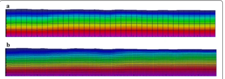
The mesh is built based on a divided rectangular triangulation (divided to make each mesh cell close to a square), and further globally refined and transformed to fit the topography of the surface. As a result, a global refinement value defines the model resolution. Simulations with a global refinement value of 6 have a cell size of approxi-mately 200 m × 200 m, while simulations with a global refinement of 7 have a cell size of approximately 100 m × 100 m, effectively quadrupling the resolution, however, requir-ing more time to compute. In practice, an increased resolution rendered by a global refinement value of 7 does not seem to have noticeable changes on the results.
Two examples of low global refinements for thermal profile 2, showing the subdivided grid and its impact on the resolution of the model, are shown in Fig. 4.
Monte Carlo method
Large uncertainties exist in thermal conductivity and heat production rate measure-ments; a Monte Carlo approach is introduced to study how those uncertainties affect thermal structure results. The fast computing time for individual model allows us to carry out more than one thousand Monte Carlo simulations easily for each 2D profile.
Monte Carlo simulations were performed utilising a Python script. An initial script was written to create directories with respect to the root configuration file and data files (which contain H and K values, with standard deviations). A total of one thousand direc-tories were generated, all of which have randomly selected thermal conductivity values, from a Gaussian distribution with measured means and standard deviations, based on laboratory measurements for each lithology. Once a simulation suite has completed, the output from all one thousand directories is compiled into singular plot files. Each plot file shows the mean, while adding and subtracting one standard deviation to show the uncertainty range. A geotherm is taken every 10 km along each profile. Extracted geotherms provide a quantitative temperature range useful for determining the ther-mal arrangement of each profile. The first iteration benchmark was set to 100; however, 100 iterations lacked the statistical rigour to apply it to all models. Increased iterations (10,000) per simulations were used to determine whether more iterations necessarily mean increased accuracy, as large simulations are computationally expensive and time-consuming process. However, no significant difference was found in the uncertainty range between 1000 and 10,000 iterations, and as a result 1000 iterations were set for all Monte Carlo simulations.
Physical model set‑up
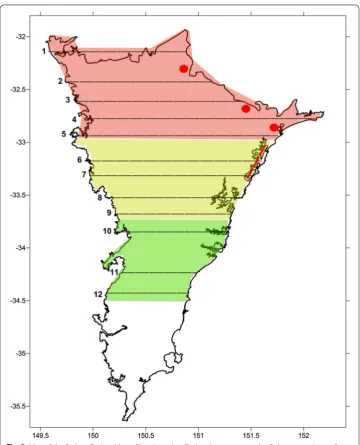
The full geological model is constructed as a series of 12 geological profiles, which define the geometry of the major lithological units for all modelled profiles. An aerial map of the area of study is shown in Fig. 5.
Boundary conditions
A surface temperature of 15 °C is used, as indicated by Danis et al. (2012). This value is taken from Cull (1979) measurements. A bottom temperature of 350 °C at 12 km is used, which is the modelled temperature used by Danis et al. (2012) in their models. Side conditions of the model have no heat flow, meaning that boundary temperatures are all accounted for at the top and bottom of the model. Excluding heat flow from side conditions ensures that the model is internally consistent by minimising edge effects. A 3rd order Lagrange interpolating polynomial was used to obtain a complete distribution between data points for multiple datasets (Liu and Gu 2001).
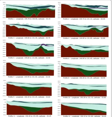
Profile geometry
bottom of the basement is not depicted in the following profiles; however, simulations assume a basement limit of 12 km—as shown in the following figures (Profiles 1–12) which have an E–W orientation (Lemenager and O’Neill 2016) (Fig. 6).
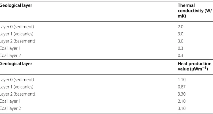
Heat production values
Heat production values have been taken from two prominent sources. Facer et al. (1980) provides a short list of packages from the Southern Coalfields in NSW and Blevin et al. (2010). Vila et al. (2010) offers a range of heat production values for common lithological groups, but does not offer site-specific values that are provided by Facer et al. (1980) and
Blevin et al. (2010). Approximated heat production values of Triassic sedimentary rocks, igneous intrusions/dykes that have been identified as intrusions of coal measures, and Permian coal measure sedimentary rocks were sampled by Facer et al. (1980). A number of the Permian samples have been recognised as inter-seam clastic rocks with varying heat production values; as a result, this represents an average between the organic and non-organic component of Permian sedimentary packages.
Although reported values are based on a limited number of samples and that it is assumed that heat production values remain constant within defined layers or packages, they provide a general idea of the large-scale heat production of pre-defined lithological packages studied in this project. Heat production values were collected via XRF (X-ray fluorescence) analysis of K and Th and U via NAA (neutron activation analysis).
A large compilation of heat production measurements were provided by Vila et al. (2010), showing a mean and percentile difference of heat production values. Reported
values vary significantly with standard deviations in some instances exceeding the mean. It was shown by Vila et al. (2010) that it is difficult to approximate and nominate specific values to a group of lithologies. Heat production values vary with location, and in order to keep value distributions manageable—taking the mean is established to be the most effective approximation, and provides a relatively realistic representation of true values. This method was then applied to the following study.
Blevin et al. (2010) provides a compiled dataset of heat production values of the Syd-ney Basin Gulgong, Bathurst and Oberon Granites representing a large number of the Lachlan Fold Belt Carboniferous Granitoids. At the current resolution of simula-tions, heat production values cited in papers above were averaged across all layers for simplicity.
Facer et al. (1980) referenced specimens are close to our area of interest, so we adopt these estimates, taking into account the uncertainty in the measurements. As a result, the following values were used, in conjunction with Blevin et al. (2010) basement esti-mates (Table 1).
Results
Thermal conductivity measurements
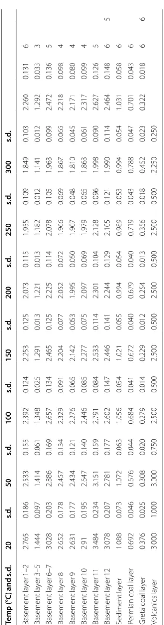
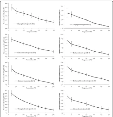
Thermal conductivity values used for this study are shown in Tables 2 and 3. These include basement thermal conductivities, compiled from Evans’s (2013) Lachlan Fold Belt Granites measurements (Additional file 1: Tables S2 and S5), and new measure-ments on Sydney Basin sedimeasure-ments (Additional file 1: Tables S3, S4 and S6). The Lachlan Belt Granites are representative of a number of granitic bodies which extend down to the Sydney Basin basement (Evans 2013). The thermal conductivity of each profile was calculated by taking the average of surrounding granites corresponding to the latitude of each thermal profile. The granites follow the same trend in thermal conductivity as depicted by Sass et al. (1992), roughly following a near-linear trend-line reducing in value, which can be useful in providing approximations as long as at least one tempera-ture-specific thermal conductivity is known, by simply applying a gradient. The thermal
Table 1 Heat production values used for geothermal models and geotherms
Geological layer Thermal
conductivity (W/ mK)
Layer 0 (sediment) 2.0
Layer 1 (volcanics) 3.0
Layer 2 (basement) 3.0
Coal layer 1 0.3
Coal layer 2 0.3
Geological layer Heat production
value (μWm−3)
Layer 0 (sediment) 1.10
Layer 1 (volcanics) 0.87
Layer 2 (basement) 3.30
Coal layer 1 2.10
conductivity, for a given temperature, of the Triassic sediment, coal measures and vol-canics were grouped as one unit type across all thermal profiles as these measurements do not possess the same degree of coverage as the granites.
Temperature-dependent thermal conductivity of sediment and coal measures meas-urements were taken in 2014 as part of this study (Lemenager and O’Neill 2016). Vol-canics thermal conductivities are recommended temperature-dependent estimates taken from Danis et al. (2012). Constant thermal conductivity values were taken from Facer et al. (1980), and basement value from Danis et al. (2012) (Figs. 7, 8).
Thermal modelling
Non-temperature-dependent thermal profiles are much more susceptible to temperature variation with depth than temperature-dependent thermal profiles. Here, non-tempera-ture dependent refers to thermal conductivity remaining constant at all temperanon-tempera-tures. Each geological layer is attributed a single thermal conductivity value which remains constant with temperature and therefore depth. As a result, geology and profile geom-etry are the main controls of temperature variation in non-temperature-dependent ther-mal profiles. The 150 °C isotherm shown in temperature-dependent therther-mal profiles (Fig. 9) are much more linear and instead gradually respond to geology and geometry. The temperature distribution in temperature-dependent thermal profiles is by com-parison smoother. Non-temperature-dependent thermal profiles (Fig. 10) persistently have thermal anomalies in close proximity to the surface as demonstrated by the 150 °C isotherm, most considerably in profiles 1–6. Thermal anomalies in profiles 1–6 may be due to the nature of the coal measures, where they are thickest in the north and reduce in thickness as it progresses south. The highly thermally resistive nature of the Greta coal could also significantly contribute to this in non-temperature-dependent thermal profiles.
Additionally, approximately ~ 35 km along thermal profile 3, the effect of topography can be seen where a local increase in sedimentary cover, as well as coal, provides further insulation. The top of the basement in the western half of thermal profile 3 is very shal-low in comparison with the eastern half. Although as seen in profile 2, high tempera-tures are associated with sediment and coal thickness, but also distance to the top of the basement from heat generation through radioactive decay of heat-producing elements. Although there is prominent topographic variation in profile 3, the resulting incongru-ence in topography, sedimentary cover, coal thickness and distance to basement ensues little disparity in temperature laterally, across the thermal profile. This profile is an
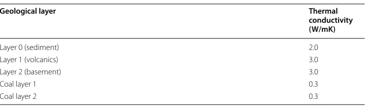
Table 2 Constant thermal conductivity values used for geothermal models
Geological layer Thermal
conductivity (W/mK)
Layer 0 (sediment) 2.0
Layer 1 (volcanics) 3.0
Layer 2 (basement) 3.0
Coal layer 1 0.3
Table 3 T emp er atur e-dep enden
t thermal c
onduc
tivit
y v
alues used in geothermal mo
dels and geotherms
sd
. r
ef
ers t
o the alloca
ted standar d devia tion Temp (°C ) and s .d . 20 s. d. 50 s. d. 100 s. d. 150 s. d. 200 s. d. 250 s. d. 300 s. d. Basement la yer 1–2 2.765 0.186 2.533 0.155 2.392 0.124 2.253 0.125 2.073 0.115 1.955 0.109 1.849 0.103 2.260 0.131 6 Basement la yer 3–5 1.444 0.097 1.414 0.061 1.348 0.025 1.291 0.013 1.221 0.013 1.182 0.012 1.141 0.012 1.292 0.033 3 Basement la yer 6–7 3.028 0.203 2.886 0.169 2.657 0.134 2.465 0.125 2.225 0.114 2.078 0.105 1.963 0.099 2.472 0.136 5 Basement la yer 8 2.652 0.178 2.457 0.134 2.329 0.091 2.204 0.077 2.052 0.072 1.966 0.069 1.867 0.065 2.218 0.098 4 Basement la yer 9 2.631 0.177 2.434 0.121 2.276 0.065 2.142 0.053 1.995 0.050 1.907 0.048 1.810 0.045 2.171 0.080 4 Basement la yer 10 2.91 0.195 2.647 0.140 2.446 0.085 2.277 0.075 2.097 0.069 1.979 0.065 1.863 0.061 2.317 0.099 4 Basement la yer 11 3.484 0.234 3.151 0.159 2.791 0.084 2.533 0.114 2.301 0.104 2.128 0.096 1.998 0.090 2.627 0.126 5 Basement la yer 12 3.078 0.207 2.781 0.177 2.602 0.147 2.446 0.141 2.244 0.129 2.105 0.121 1.990 0.114 2.464 0.148 6 5 Sediment la yer 1.088 0.073 1.072 0.063 1.056 0.054 1.021 0.055 0.994 0.054 0.989 0.053 0.994 0.054 1.031 0.058 6 Per
mian coal la
yer 0.692 0.046 0.676 0.044 0.684 0.041 0.672 0.040 0.679 0.040 0.719 0.043 0.788 0.047 0.701 0.043 6 Gr
eta coal la
example of the effect of complex geometry on the thermal structure of the Sydney Basin, and highlights the requirement for the understanding of large-scale geology.
It can be concluded that temperature-dependent and non-temperature-dependent thermal profiles distinctively vary from each other. Geothermal gradients between the two sets of models (temperature dependent and non-temperature dependent) at times exhibit rather large temperature discrepancies; for example, profile 4 point 9 (80 km along the profile) has up to 50 °C difference in temperature, and in geothermal explora-tion this is a substantial temperature gap. In sum, temperature field variaexplora-tion between temperature-dependent and non-temperature-dependent thermal profiles are suf-ficiently significant to infer that temperature-dependent thermal conductivity has an important impact in the way heat is distributed in the Sydney Basin (Lemenager and O’Neill 2016).
Geotherms
In order to assess the uncertainty in our calculated downhole temperature, we utilised a Monte Carlo approach. We assigned Gaussian distributions to our temperature-dependent conductivity, based on the means and standard deviations of the tempera-ture-dependent conductivity curves shown in “Thermal conductivity measurements” section.
The output statistical variation is shown on geotherm plots, extracted from tempera-ture-dependent thermal profiles. A series of geotherms at 1000 iterations were plotted
Fig. 8 Thermal conductivity of sedimentary/coal rocks. Sediment layers are an average value of Triassic Sydney Basin sediments—consisting of coastal samples such as conglomerates, muddy sandstone and medium-grained sandstone. Permian coal layer is an average of the Whittingham, Tomago and Newcastle coal measures (Volcanics layer is an artificial value adapted from Danis et al. (2012) models, values are listed in Table 2)
showing uncertainties in temperature with depth (Fig. 11). It can be noted that each plot converges to 0 uncertainties as they meet the default boundary conditions.
The 150 °C isotherm occurs between depths of 1500 and 4303 m across all profiles (Table 3). Bold markers show minimum uncertainties within 2 km from the surface and may be areas of interest regarding the potential for geothermal energy in the Sydney Basin.
Geothermal gradients by Danis et al. (2012) are based on measured equilibrated bore-hole groundwater from approximately 500 m downbore-hole. The extrapolated temperature uncertainty from these measurements is shown in Fig. 12 as purple polygons. In con-trast, the geothermal gradients produced in this study are based on non-linear temper-ature-dependent thermal conductivity measurements and their associated uncertainties based on variations in thermal conductivity.
The projected temperatures presented here (Fig. 11) exhibit a consistent incongruity in relation to borehole temperature data shown as purple polygons, which apply to shal-low depths based on Danis et al. (2012) measurements. However, the polygons and trend lines in Fig. 11 do not correspond to the same exact location, as thermal models were designed based on known topography cross cutting the Sydney Basin, and therefore are only within proximal range of dedicated groundwater borehole data points. Therefore, the level of correlation between each dataset can be inferred to be relatively low. Never-theless, this apparent divergence can be used as diagnostic for establishing a comparison between simulations and measurements (Table 4).
Discussion
Importance of temperature‑dependent thermal conductivity
Constant and temperature-dependent thermal profiles indicate that thermal conductiv-ity has an important impact on subsurface temperature distributions. Thermal profiles
Fig. 10 Non-temperature-dependent (constant) thermal conductivity models for profiles 1–12. Temperature is given in degrees Kelvin (range from 288 to 623 K). K-NTD refers to K thermal conductivity and NTD
using constant thermal conductivity respond very closely to basin geometry, while tem-perature-dependent thermal profiles display a gradual change in geothermal gradient with depth.
While the effect of additional variables such as pressure and pore size is not accounted for in our thermal models, the effect of thermal conductivity in geothermal model-ling looks to be of great importance (Abdulagatova et al. 2009); Triassic sediments are assumed to exhibit sufficient compaction. However, in the case of high porosity, this fea-ture can be deemed more significant than solid thermal conductivity, as fluid thermal conductivity will begin to play an increasingly important role.
Crustal thermal modelling at relatively extensive depths (e.g. down to the Moho dis-continuity, approximately 35 km) would benefit from representative thermal conduc-tivity values (Vosteen and Schellschmidt 2003), and given the sensitivity we have seen in the range of 20–300 °C, representative values may not currently exist. The crust is
Table
4
150 °C geotherm distributions a
t 10-k
m in
ter
vals f
or each geothermal pr
ofile
Pr
ofile 1 (a
v. 255 m)
Pr
ofile 2 (a
v. 389 m)
Pr
ofile 3 (a
v. 193 m)
Pr
ofile 4 (a
v. 317 m)
Pr
ofile 5 (a
v. 132 m)
Pr
ofile 6 (a
v. 318 m) Point 0 3156–3466 m Point 0 3993–4303 m Point 0 3063–3166 m Point 0 3114–3250 m Point 0 3095–3173 m Point 0 3192–3605 m Point 1 3116–3400 m Point 1 3838–4096 m Point 1 2934–3063 m Point 1 2934–3063 m Point 1 3093–3190 m Point 1 2934–3373 m Point 2 3027–3337 m Point 2 3734–3993 m Point 2 2779–2908 m Point 2 2675–2779 m Point 2 3073–3170 m Point 2 2753–3179 m Point 3 3002–3260 m Point 3 3476–3708 m Point 3 2546–2701 m Point 3 2210–2417 m Point 3 2804–2934 m Point 3 2275–2688 m Point 4 2924–3105 m Point 4 3176–3460 m Point 4 2494–2649 m Point 4 2469–2727 m Point 4 2598–2675 m Point 4 2017–2417 m Point 5 2959–3140 m Point 5 2882–3166 m Point 5 2572–2701 m Point 5 2572–2830 m Point 5 2494–2649 m Point 5 1810–2004 m Point 6 3063–3269 m Point 6 3011–3347 m Point 6 2391–2546 m Point 6 2804–3373 m Point 6 2753–2856 m Point 6 1952–2159 m Point 7 3037–3295 m Point 7 2779–3192 m Point 7 2698–2779 m Point 7 3037–3502 m Point 7 2882–3089 m Point 7 1926–2120 m Point 8 2804–3037 m Point 8 2365–2830 m Point 8 2804–3037 m Point 8 3140–3683 m Point 8 2753–3062 m Point 8 2042–2210 m Point 9 2830–3063 m Point 9 2184–2675 m Point 9 2779–3063 m Point 9 2986–3502 m Point 9 2946–3063 m Point 9 2030–2223 m Point 10 2779–3114 m Point 10 1952–2494 m Point 10 2882–3140 m Point 10 2959–3269 m Point 10 2895–3037 m Point 10 2055–2456 m Point 11 3089–3399 m Point 11 1926–2520 m Point 11 3311–3543 m Point 11 2624–2908 m Point 11 3321–3411 m Point 11 2068–2469 m Point 12 1926–2443 m Point 12 3046–3305 m Point 12 2649–2934 m Point 12 3437–3541 m Point 12 2042–2456 m Point 13 1823–2339 m Point 13 3192–3450 m Point 13 3037–3399 m Point 13 3269–3386 m Point 13 2197–2391 m Point 14 3476–3708 m Point 14 3424–3889 m Point 14 2262–2533 m Point 15 3295–3734 m Point 15 1862–1978 m Point 16 3063–3450 m Point 16 2559–2624 m Point 17 3011–3192 m Point 17 2804–2908 m Point 18 3218–3347 m Point 18 2817–2946 m Pr
ofile 7 (a
v. 271)
Pr
ofile 8 (a
v. 206 m)
Pr
ofile 9 (a
v. 99 m)
Pr
ofile 10 (a
v. 128 m)
Pr
ofile 11 (a
v. 233 m)
Pr
ofile 12 (a
Table 4 (c on tinued) Pr
ofile 7 (a
v. 271)
Pr
ofile 8 (a
v. 206 m)
Pr
ofile 9 (a
v. 99 m)
Pr
ofile 10 (a
v. 128 m)
Pr
ofile 11 (a
v. 233 m)
Pr
ofile 12 (a
v. 109 m) Point 6 1978–2146 m Point 6 2662–2946 m Point 6 2546–2675 m Point 6 2430–2572 m Point 6 2365–2456 m Point 7 2107–2301 m Point 7 2611–2817 m Point 7 2417–2520 m Point 7 2482–2585 m Point 8 2301–2456 m Point 8 2533–2675 m Point 8 2404–2486 m Point 8 2546–2637 m Point 9 2314–2469 m Point 9 2714–2843 m Point 9 2598–2662 m Point 10 2301–2443 m Point 11 2197–2365 m Point 12 2120–2288 m Point 13 2262–2430 m Range w as e xtr apola ted fr om geother mal g radien t plots . I talic poin ts r ef er t o r eg ions abo ve 2 k m, and ‘a v.’ v alue r ef ers t
o the a
ver
age diff
er
enc
e in depth bet
w
een pr
ofiles and their r
espec
tiv
e poin
host to a large variety of rock types which all have very different thermal conductivities (Clauser and Huenges 1995), mineralogical and structural complexities which can lead to anisotropy in thermal conductivity (Goff and Holliger 2012).
Temperature-dependent thermal profile 2 exhibits a very distinct temperature distri-bution mainly caused by the insulating thermal properties of the Permian and Greta coal measures, as confirmed by Sass et al. (1992) interpretations of the negative correlation between thermal conductivity and thermal gradient. While constant thermal conductiv-ity thermal profiles have irregular temperature distributions and shallower 150 °C iso-therms, as portrayed in Fig. 10, incorporating constant thermal conductivities in thermal models has highlighted the disparity between constant and temperature-dependent ther-mal models. Therther-mal another-malies associated with constant therther-mal conductivity therther-mal models could lead to misleading interpretations of the thermal structure of the Sydney Basin. Figure 13 demonstrates the temperature difference between constant and tem-perature-dependent thermal profiles, beneath a thick sequence of the Greta coal meas-ures. The constant thermal conductivity curve (in black) infers a temperature 150 °C at less than 1 km, whereas the temperature-dependent thermal conductivity curve infers a temperature of 150 °C at approximately 4 km. This large offset is a strong example of the relevance of temperature-dependent thermal conductivity. It should be noted that while
there are very limited freely available thermal conductivity data (McKenna et al. 1996), much less for location-specific temperature-dependent measurements, it should be noted that reliable prognostics to verify the real-world applications of TP–TC are scarce. To verify the potential usefulness of such thermal models would require probing the temperatures at depth at specific locations matching that of geotherms presented here.
Importance of coal
The quantitative impact of coal measures in basin thermal structure is not entirely understood; however, it is known to some degree that sediments generally act as ther-mal insulators or ‘therther-mal blankets’ (Lucazeau and Le Douaran 1985). Danis et al. (2012) and Danis (2014) capitulate that coal-bearing sedimentary basins have largely been over-looked in their ability to provide sufficient insulation as to be considered precursors for geothermal resources. The presence of thick coal measures in the Sydney basin (Jones et al. 1987) has a noticeable impact on the thermal structure of the Sydney Basin as sug-gested by the discrepancy in thermal fields in TD and non-TD thermal conductivities (Fig. 9) in the shallow crust (within 3–4 km). Relatively elevated geotherms coincide with areas of thick coal measures and the proximity of those coal measures to the surface. The apparent effect of thermal insulation caused by the Sydney Basin coal measures results in an overall rise in the temperature field underneath those coal measures, despite exhib-iting relatively low surface heat flux (Rawling et al. 2014).
The second thermal profile (in Fig. 9) is a great example of the disparity in temperature distribution between a region of very low sedimentary cover with no coal (west side) and a region of very thick sedimentary cover (East side—up to 3000 m) with thick Permian coal layers and a very thick Greta coal layer which has extremely insulating thermal con-ductivities (~ 0.3 W/mK). Thermal profile 2 provides a direct correlation between thick sedimentary cover and coal measures, and a shallow 150 °C isotherm. The lack of sedi-mentary cover at the beginning of the profile (up to 80 km along the profile line) results in basement heat being refracted up to this low-conductivity pathway. Thermal profile 4 exhibits two comparatively low-temperature geotherms (at 80 and 145 km along the profile line), which correlate with reduced coal thickness and increased distance to top of basement.
The 150 °C isotherm is elevated beneath thick coal measures, as demonstrated in Fig. 9. However, another significant effect is the thickness of the basin sediments and the relative depth to the top of the basement. Profile 5 has especially high geotherm temperatures beneath the coal (600 m beneath surface) at 140 km along the profile line, where the Greta coal measure is at its thickest (approximately ~ 750 m thick). This ther-mal another-maly is directly caused by the presence of insulating coal, where the temperature profile is otherwise relatively linear.
Effect of basin and basement geometry on thermal model
The model is defined by basin and basement geometry, and the physical properties bound to the geology. Variation of top basement geometry in turn affects the subsur-face variation in thermal conductivity itself as a function of depth and temperature. Therefore geometry, and topography, has a significant effect on the thermal structure of the Sydney Basin (Danis et al. 2012).
Thermal profile 3 addresses the importance of basin geometry through topography, where at approximately ~ 35 km along the profile line, high topography has resulted in a local increase in sedimentary cover, together with coal providing additional insu-lation. The top of the basement within the western half of thermal profile 3 is very shallow in comparison with the eastern half of the profile. Again, elevated 150 °C isotherms are associated with both sediment and coal thickness, and distance to the top of the basement. The latter effect is a function of both the high concentration of radiogenic elements in the basement rocks, generating significant heat (Blevin et al.
2010), and the relatively high conductivity of crystalline basement.
Although there is prominent topographic variation in profile 3, the competing effects of topography, sedimentary cover, coal thickness and distance to basement ensue little disparity in temperature laterally, across the thermal profile. This profile is an example of the effect of complex geometry on the thermal structure of the Syd-ney Basin, and highlights the importance of understanding of large-scale geology of a basin.
Conclusions
The initial aims of this study have been to compile and incorporate the basin geom-etry and temperature-dependent thermal conductivity measurements and constant thermal conductivity values in thermal models of the Sydney Basin, and assess their relevance in terms of their effect on thermal structure.
Authors’ contributions
AL co-wrote the manuscript, performed the simulations and conducted the experiments. SZ co-wrote the manuscript and developed the code. CO co-wrote the manuscript and assisted with the experiments and sampling. ME performed some experiments and sampling. All authors read and approved the final manuscript.
Acknowledgements
I would like to sincerely thank my supervisors, Craig O’Neill and Siqi Zhang who have taught me a lot and guided me through the world of academic research. I thank my peers, friends and family for their constant support. Funding pro-vided by ARC/CCFS is abundantly acknowledged.
Competing interests
The authors declare that they have no competing interests. Availability of data and materials
Data are available upon request. Consent for publication
All co-authoring parties consent to the publication of the material. Ethics of approval and consent to participate
No ethics of approval is required. Funding
Craig O’Neill (C.O.), Siqi Zhang (S.Z.), Morgan Evans (M.E.) and Alexandre Lemenager (A.L.) acknowledge ARC/CCFS funding.
Publisher’s Note
Springer Nature remains neutral with regard to jurisdictional claims in published maps and institutional affiliations.
Received: 6 December 2017 Accepted: 17 April 2018
References
Abdulagatova Z, Abdulagatov IM, Emirov VN. Effect of temperature and pressure on the thermal conductivity of sand-stone. Int J Rock Mech Mining Sci. 2009;46(6):1055–71.
Bangerth W, Hartmann R, Kanschat G. deal. II—a general-purpose object-oriented finite element library. ACM Trans Math Softw (TOMS). 2007;33(4):24. https ://www.deali i.org.
Blevin P, Chappell B, Jeon H. Heat generating potential of igneous rocks within and underlying the Sydney Basin: some preliminary observations. In: Proceedings of the 37th symposium of the geology of the Sydney Basin. 2010. Casareo F. Geochemical and petrographic studies of coals in the upper Permian Whittingham coal measures, Northern
Sydney Basin, NSW, Australia. North Ryde: Macquarie University; 1996.
Clauser C, Huenges E. Thermal conductivity of rocks and minerals. In: Ahrens TJ, editor. Rock physics & phase relations: a handbook of physical constants. Washington: American Geophysical Union; 1995. p. 105–26.
Conaghan PJ, Jones JG, McDonnell KL, Royce K. A dynamic fluvial model for the Sydney Basin. J Geol Soc Aust. 1982;29(1–2):55–70.
Cull JP. Climatic corrections to Australian heat-flow data. BMR J Aust Geol Geophys. 1979;4:303–7.
Danis C. Use of groundwater temperature data in geothermal exploration: the example of Sydney Basin. Australia. Hydro-geol J. 2014;22(1):87–106.
Danis C, O’Neill C. A static method for collecting temperatures in deep groundwater bores for geothermal exploration and other applications. In: Proceedings of Groundwater. 2010.
Danis C, O’Neill C, Lackie M, Twigg L, Danis A. Deep 3D structure of the Sydney Basin using gravity modelling. Aust J Earth Sci. 2011;58(5):517–42.
Danis C, O’Neill C, Lee J. Geothermal state of the Sydney Basin: assessment of constraints and techniques. Aust J Earth Sci. 2012;59(1):75–90.
Additional file
Evans M. Thermal conductivity database of Paleozoic instrusives of Basement to the Sydney Basin. Sydney: Department of Earth and Planetary Sciences, Macquarie University; 2013.
Facer RA, Cook AC, Beck AE. Thermal properties and coal rank in rocks and coal seams of the Southern Sydney Basin, NSW: a palaeogeothermal explanation of coalification. Int J Coal Geol. 1980;1(1):1–17.
Goff JA, Holliger K, editors. Heterogeneity in the crust and upper mantle: nature, scaling, and seismic properties. Berlin: Springer Science & Business Media; 2012. p. 348.
Gulson BL, et al. High precision radiometric ages from the northern Sydney Basin and their implication for the Permian time interval and sedimentation rates. Aust J Earth Sci. 1990;37(4):459–69.
Heller PL, Angevine CL, Winslow NS, Paola C. Two-phase stratigraphic model of foreland-basin sequences. Geology. 1988;16(6):501–4.
Herbert C. Sequence stratigraphy of the Late Permian coal measures in the Sydney Basin. Aust J Earth Sci. 1995;42(4):391–405.
Hunt J, Anderson A, Benett A, Brakel A, Whithouse J. Petrography and geochemistry of the coals and depositional environments of the sediments in the late Permian Tomago and Newcastle coal measures from the bore Strevens Terrigal 1—Northern Eastern Sydney Basin, NSW. North Ryde: CSIRO-Institute of Energy and Earth Resources; 1984. Jones JG, Conaghan PJ, McDonnell KL. Coal measures of an orogenic recess: late Permian Sydney Basin. Australia.
Palaeo-geogr Palaeoclimatol Palaeoecol. 1987;58(3–4):203–19.
Lemenager A, O’Neill C, Zhang S, Evans M. Numerical modelling of the Sydney Basin using temperature dependent ther-mal conductivity measurements. In: ASEG-PESA-AIG 25th Geophysical conference and exhibition, Adelaide. 2016. Liu GR, Gu Y. A point interpolation method for two-dimensional solids. Int J Numer Methods Eng. 2001;50(4):937–51. Lucazeau F, Le Douaran S. The blanketing effect of sediments in basins formed by extension: a numerical model.
Applica-tion to the Gulf of Lion and Viking graben. Earth Planet Sci Lett. 1985;74(1):92–102.
McKenna TE, Sharp JM Jr, Lynch FL. Thermal conductivity of Wilcox and Frio sandstones in south Texas (Gulf of Mexico Basin). AAPG Bull. 1996;80(8):1203–15.
Middleton MF, Schmidt PW. Paleothermometry of the Sydney Basin. J Geophys Res Solid Earth. 1982;87(B7):5351–9. Moresi L, et al. Computational approaches to studying non-linear dynamics of the crust and mantle. Phys Earth Planet
Interior. 2007;163(1–4):69–82.
Nabelek PI, Hofmeister AM, Whittington AG. The influence of temperature-dependent thermal diffusivity on the conduc-tive cooling rates of plutons and temperature-time paths in contact aureoles. Earth Planet Sci Lett. 2012;317:157–64. Noack V, Scheck-Wenderoth M, Cacace M. Sensitivity of 3D thermal models to the choice of boundary
condi-tions and thermal properties: a case study for the area of Brandenburg (NE German Basin). Environ Earth Sci. 2012;67(6):1695–711.
Rawling TJ, Sandiford M, Beardsmore GR, Quenette S, Goyen SH, Harrison B. Thermal insulation and geothermal targeting, with specific reference to coal-bearing basins. Aust J Earth Sci. 2014;60:817–29.
Ryskin A, Pleiner H. Influence of sedimentation on convective instabilities in colloidal suspensions. Int J Bifurcation Chaos. 2010;20:225.
Sass JH, Lachenbruch AH, Moses TH, Morgan P. Heat flow from a scientific research well at Cajon Pass, California. J Geo-phys Res Solid Earth. 1992;97(B4):5017–30.
Shuttle Radar Topography Mission: United States Geological Survey. 2015. http://www2.jpl.nasa.gov/srtm/cband -datap roduc ts.html. Accessed June 2015.
Vila M, Fernandez M, Jimenez-Munt I. Radiogenic heat production variability of some common lithological groups and its significance to lithospheric thermal modelling. Technophysics. 2010;490(5):152–64.