R E S E A R C H A R T I C L E
Open Access
A simple and unified implementation of
phase field and gradient damage models
E. Azinpour, J. P. S. Ferreira, M. P. L. Parente and J. Cesar de Sa
∗*Correspondence: [email protected]
INEGI-Institute of Science and Innovation in Mechanical and Industrial Engineering, University of Porto, Rua Dr. Roberto Frias, 4200-465 Porto, Portugal
Abstract
In this work, the analogous treatment between coupled temperature–displacement problems and material failure models is explored within the context of a commercial software (Abaqus®). The implicit gradient Lemaitre damage and phase field models are implemented utilizing the software underlying capabilities for coupled
temperature–displacement problems. The heat conduction equation is made compatible with the diffusive regularization of such material models and calculations are carried out at the material point level. This bypasses the need to implement explicitly the weak form resultant from the coupling between the momentum conservation and the evolution of the diffusive field. Throughout benchmarking examples, the proposed methodology is assessed and validated by investigating typical issues risen from the considered local inelastic-based deformation models, such as mesh dependency and the difficulties to predict cracked regions.
Keywords: Material failure, Commercial software, Implicit gradient Lemaitre damage model, Phase field model, Diffusive regularization, Mesh dependency
Introduction
The emergence of the so-called ‘regularized’ solutions for damage and failure in engi-neering materials has evolved considerably in recent years. They constitute appealing simplifications of the microstructural complexity, usually resorting to non-local and gra-dient theories. To ensure well-posedness of the set of partial differential equations to be solved, which is affected by the presence of softening at the constitutive level, these solu-tions abandon the principle of local action by coupling a diffusion equation of non-local variables with the momentum balance equation. The resultant procedure acts as a spa-tial regularization of local constitutive relations for failure, usually with the recourse of a characteristic length associated with the size of the non-local support region definition. Herein, two types of regularization are explored, namely: the non-local implicit gradient of the Lemaitre damage model [1] and the phase field model [2] that approximate crack evolution under inelastic deformations.
Prediction of initiation and propagation of cracks defines a highly crucial task in behav-ior assessment of ductile metallic structures, which requires the development of accurate and robust constitutive models that trigger the formation of meso-cracks initiated by the material internal progressive degradation due to nucleation, growth, and coalescence of microvoids. Within the context of coupled models, which take into account that
degra-©The Author(s) 2018. This article is distributed under the terms of the Creative Commons Attribution 4.0 International License (http://creativecommons.org/licenses/by/4.0/), which permits unrestricted use, distribution, and reproduction in any medium, provided you give appropriate credit to the original author(s) and the source, provide a link to the Creative Commons license, and indicate if changes were made.
dation continuously coupled with the evolving deformation, two major methodologies are commonly adopted: micromechanical or continuous damage mechanics approaches. The micromechanical-based methodologies include at the constitutive level the effect of internal degradation through material parameters calibrated with a set of experimental tests. Many were inspired on the early work of Rice and Tracey [3], that focused primarily on the microscopic evolution of a spherical void in a rigid perfectly-plastic matrix of the material, and later on the work of Gurson [4], followed by the work of Tvergaard and Needleman [5] that represent internal degradation as a volume void fraction (porosity). Another insight derived from the Continuum Damage Mechanics approach, built over the concepts defined in the seminal work of Kachanov [6], which defines the internal thermodynamically-consistent damage field phenomenologically continuously evolving to a threshold value, was firstly introduced by Lemaitre and Chaboche in [7–9]. Numeri-cal implementations soon followed, both in the context of small strain [10] and large strain [11] analyses.
Local continuum description of damage typically may lead to an ill-posed boundary value problem as under a softening regime the governing partial differential equations may locally lose their ellipticity or change its hyperbolic character, in static and dynami-cal problems, respectively. This may result in mesh (geometridynami-cal discretization) sensitive solutions, where the localized zones and internal variables are highly dependent on the mesh size and discretization alignment. To avoid these inconsistencies and restore mesh objectivity, non-local approaches may be adopted by adding regularization or averaging procedures associated with a length scale effect, whether via an integral-based non-local methodology, as in Pijaudier-Cabot and Bažant [12] or gradient-type non-local meth-ods, as in Peerlings et al. [13]. The latter has been utilized in many contexts, namely, in quasi-brittle fracture [14,15], small strain [16] and finite strain elastoplasticity [17], finite strain elastoplasticity coupled with damage [18] or in ductile damage frameworks [19,20], referring only to some more recent contributions.
Another type of regularization, known as the phase field method, originally departing from fracture mechanics concepts, aims to assess the evolution of macrocracks in a diffu-sive topology using methodologies associated with phase transition. Its implementation in the context of the finite element method allows for the possibility of tracking the cracks without any modification in the mesh grid lines which is still an utmost issue in the discrete crack approaches. The genesis of this concept was founded in the variational description of brittle fracture by Francfort and Marigo [21] and eliminates the requirement to describe a well-defined crack path. The concept was extended by the regularization approach of Bourdin et al. [22] and by the-convergent approximations of Mumford and Shah [23].
et al. [35], the phase field elastoplastic models by Duda et al. [36] and Ambati et al. [37], the crystal plasticity phase field coupled model of Padilla et al. [38], the phase field based anisotropic damage model of Mozaffari et al. [39] and the variational based, large defor-mation plasticity-phase field model by Miehe et al. [40,41] and rate-dependent plasticity phase field model of Badnava et al. [42] mostly concentrated on approximating the post-peak material behavior via a phase field methodology. Also in [43], de Borst et al. studied several similar and different aspects of gradient enhanced damage-based approaches and the phase field framework and a discussion has made over the solution of the broadening of the damaged zone in the wake of the crack tip with these methods.
The present study addresses a methodology for solving the diffusion equation of the phase field model and gradient-enhanced non-local damage model, in the context of an existing commercial software. It takes the advantage of built-in heat equation solver in an existing software code, Abaqus/Standard in the present case, bypassing the need to establish explicitly the weak form of the governing equations containing the momentum balance and the diffusion equation to solve separately for displacement and non-local or phase field variables. In fact, this procedure could be used with other commercial softwares with similar capabilities. This work is organized as follows: “Formulation” section builds the relation between the heat conduction problem and diffusion equation of gradient problems, and explains the gradient non-local model based on Lemaitre phenomeno-logical ductile damage model and the phase field model. Numerical implementation and results of some illustrative examples are presented in “Results and discussion” section, and finally conclusions are drawn in “Concluding remarks” section and a shortened version of routine to implement the non-local gradient damage model is provided.
Formulation
In both gradient damage and phase field models, the mechanical equilibrium is performed for the coupling between displacementsuand a field variableψ. In a body, the strong form of the boundary value problem can be written, in general, as
divσ+b=0
∇(Γ (a)∇ψ)=hs
in (1)
whereσis the stress tensor andbis the body force per unit of volume, with the following boundary conditions:
σ.n=tn on∂t u=ud on∂u ∇ψ.n=0 on∂
(2)
being∂ = ∂u∪∂t the body surface boundary,n outward unit normal vector to
the boundary surface at ∂t,tnthe traction force, ud prescribed displacements at the boundary surface∂uandaa set of possible material and numerical parameters. Second part of Eq. (1) depends on a “diffusion” coefficientΓ (a), on the “flux”, or gradient, term
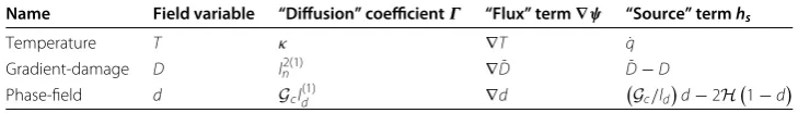
Table 1 Diffusion equation forms for coupled temperature displacement, gradient-damage, and phase-field models
Name Field variable “Diffusion” coefficientΓ “Flux” term∇ψ “Source” termhs
Temperature T κ ∇T q˙
Gradient-damage D ln2(1) ∇D¯ D¯−D
Phase-field d Gcld(1) ∇d
Gc/ld
d−2H1−d κThermal conductivity,hsheat source,lncharacteristic length for gradient damage model,Gcfracture energy,Helastic
energy density,ldcharacteristic length for phase field-model
commercial software packages in the computational mechanics field hints that it may be used in establishing gradient and phase field models within these frameworks, taking advantage of the software built-in implementations. In Table1, the parametersln and ldare respectively length parameters associated to the gradient damage and phase field approaches, commonly denoted as the characteristic length scale of the material and are mostly considered as numerical parameters. Since its meaning with the microstructure is inherently complex, its precise determination usually relies on inverse methods [44].
Lemaitre damage model coupled with plasticity
The constitutive modeling of the fully-coupled damage-plasticity model in [1] is recov-ered in this section, considering its extensive application in describing ductile damage in metallic materials. This model is often categorized within the Continuous Damage Mechanics material behavior description as the damage is phenomenologically intro-duced at the macroscopic constitutive level by internal variables whose evolution mimic the nucleation, growth and coalescence of internal micro-voids. Mostly it is based on the hypothesis of strain equivalence and the associated concept of effective stress. Herein, the simplified version of the Lemaitre thermodynamically-consistent damage model proposed by De Souza Neto et al. [45], in the context of small strains, is adopted for simplicity.
The decomposition of total strain tensor into elastic (εe) and plastic (εp) contributions yields:
ε=εe+εp (3)
Accordingly, the free energy can be stated as the sum of the elastic damageψedand plastic (ψp) potentials:
ψ =ψed(εe, D)+ψp(α) (4)
whereαis an isotropic hardening (internal) variable andDis the damage (internal) variable defined as a scalar, 0 ≤D≤1, evolving continuously from zero (virgin material) to one (fully damaged material). Assuming the elastic damage contribution as:
ψed(εe, D)= 1 2ε
e: (1−D)De:εe (5)
the constitutive law reads:
σ=∂εe(ψ)=(1−D)De:εe (6)
whereσis the Cauchy stress tensor andDeis the isotropic fourth order elasticity tensor, which may be defined as:
where GandK are respectively shear and bulk moduli,I is the second order identity tensor, Id = Is− 13I⊗I is the fourth order deviatoric projection tensor andIs is the symmetric identity tensor, given by:
Is= ⎡ ⎢ ⎣
1 0 0
1 0
sym 12
⎤ ⎥
⎦ (8)
The yield condition to define the plastically admissible stress states is defined as:
fy= ¯ σ(s)
1−D−σy(α)≤0 (9)
where ¯σ(s)=3J2(s) is the von Mises equivalent stress withJ2(s) as the second invariant of the deviatoric stress tensor,s. The yield stressσy(α) is a function of the internal hard-ening variable,α, which is considered herein as the equivalent plastic strain, ¯εp, written as:
¯ εp=
t
0
2 3ε˙
pdt (10)
where ˙εpis the rate of the plastic strain. The associative plastic flow rule is assumed and then:
˙
εp=γ˙N (11)
where ˙γ is the plastic multiplier andNis the flow vector, defined as:
N =
3 2
s
(1−D)s (12)
These relations are supplemented by the definition of damage-related energy derived from the total potential as:
Y =∂D(ψ)= −1 2ε
e:De:εe (13)
whereY is the damage energy release rate which can be alternatively written as:
Y = 1
(1−D)2
−σ¯2
6G −
p2 2K
(14)
beingp= 13tr(σ) the hydrostatic pressure. The evolution of the internal variables reads:
˙ α=γ˙
˙
D= r1
(1−D) (1+r2)
−Y
r1
r2+1 (15)
wherer1andr2are material parameters which can be calibrated by experimental observa-tions. Finally, the usual loading/unloading conditions of rate-independent plasticity follow as:
Gradient regularization of the local damage model
The non-local implicit gradient formulation is here recovered. Based on this approach, a non-local field ¯f is related to the corresponding local fieldf, as in Eq. (1), through the equation:
¯
f −ln∇2f¯=f (17)
This approach bypasses the calculation of second order gradients of the local field of explicit nonlocal models, and establishes a more robust solution. Here, we focus on the gradient regularization of Lemaitre based local damage field, resorting to an alternative numerical treatment in the context of the treatment of multi-field problem within a commercial finite element code Abaqus/Standard.
As a point of departure, the following set of governing equations defines the implicit gradient elastoplastic framework coupled with the internal damage:
divσ+b=0 ¯
D−l2nD¯ =D on (18)
which includes the stress equilibrium and the additional partial differential equation cor-responds to the implicit gradient regularization of the local damage field,D. In Eq. (18)2,
D¯ = ∇2D¯denotes the Laplacian of the nonlocal damage field. With this strong form at hand, the following homogenous Neumann boundary conditions are prescribed:
∇D.¯ n=0 on∂ (19)
Unlike the explicit gradient formulation, this boundary condition is homogenous and does not require the gradient of the local field as an additional nodal degree of freedom.
Following the constitutive relations of the previous section, the yield function of Eq. (9) can be rewritten based on the nonlocal field:
fy= ¯ σ(s)
1−D¯−σy(α) (20)
Accordingly, the flow vector may be modified as:
N =
3 2
s
1−D¯s (21)
This is followed by the rate forms of the internal hardening variable and damage parameter:
˙
α =γ˙ (22)
˙ D= γ˙
1−D¯
−Y r1
r2
(23)
together with the damage driving force written as:
Y = 1 1−D¯2
−σ¯2
6G −
p2 2K
(24)
Integration algorithm of the non-local resolution
mechanical problem is performed via the known iterative Newton Raphson algorithm to solve the return mapping equation, as is proved to have quadratic convergence rates.
Givenεand nonlocal damage variable from the previous increment ( ¯Dn) and consid-ering the pseudo time intervalt ∈(tn, tn+1), elastic predictor stage gives the following elastic trial states:
εe trial
n+1 =εen+ε
ptrialn+1=1−D¯n
Kεvne trial+1 strial
n+1=2
1−D¯n
Gεe triald n+1
¯ εp
n+1=ε¯
p n
¯ σtrial
n+1 =
3J2
strial
n+1
(25)
whereεe trialv n+1andεe triald n+1are, respectively, the trial values of elastic volumetric strain and elastic deviatoric strain tensor:
εe trial v n+1=
1 3tr
εe trial
n+1
εe trial
d n+1=εe trialn+1 −εe trialv n+1I
(26)
The plastic admissibility is evaluated by the following incremental yield function:
fy= ¯ σtrial
n+1
1−D¯n
−σyε¯pn+1≤0 (27)
If this condition is satisfied, the elastic stage proceeds by taking the trial predictor states as the updated values:
(.)n+1=(.)trial (28)
Otherwise, the single equation return mapping algorithm is activated and triggers the solution of the following equation to obtain the plastic multiplier,γ:
ωn+1−ωn+ωnγ +1
−
Y(γ) r1
r2
=0 (29)
considering the so-called material integrity in the previous and current increments as:
ωn ≡1−Dn ωn+1≡1−Dn+1=
3Gγ
¯ σtrial
n+1 −σy
¯ εp
n+γ
(30)
The damage energy release rate is given by:
−Y(γ)=
σy¯εnp+γ 2
6G +
ptrial
n+1 2
2K (31)
The Newton Raphson solution strategy is utilized to solve the Eq. (29) iteratively, taking the following initial value for the plastic multiplier rate:
γ = ωnfy
σ,D¯
By achieving the prescribed tolerance, the state variables are updated based on the new material integrity:
¯ εp
n+1=ε¯
p n+γ
pn+1=ωn+1
ptrialn+1
¯
σn+1=ωn+1σy
ε−p
n+1
sn+1= ¯ σn+1 ¯ σtrial
n+1
strial n+1
σn+1=sn+1+pn+1I
εe n+1=
1
2Gsn+1+ε e trial v n+1I
(33)
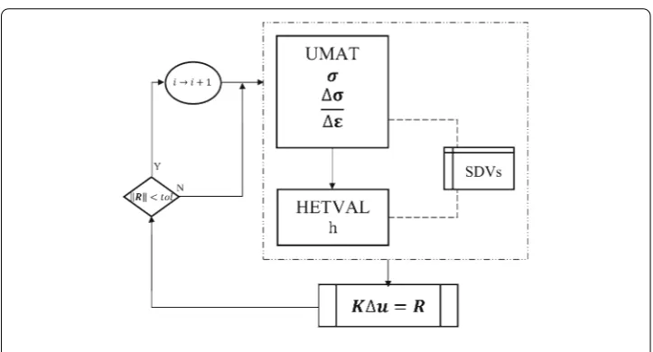
Using Abaqus/Standard as a support software, the above integration algorithm is coded into a UMAT subroutine to reach the updated stress and local damage fields. This is processed based on the nonlocal damage fields obtained from the solution of diffusion Eq. (18)2in each increment. Solution of this equation is achieved via the HETVAL subroutine, taking into consideration the similarity of this gradient regularization with the steady state heat conduction equation in solids. In fact, for convenience, in each increment the transient heat equation is used
ρcp∂tT−κ∇2T =q˙ (34)
with “thermal” constants (specific heatcpand densityρ), “pseudo time” and time incre-ment so that the steady-state conditions are closely attained in each load increincre-ment. Given the local damage field, the nonlocal solution is achieved by the following assumptions (see Table1):
κ≡ln2 ˙
q≡D−D¯ (35)
The layout of the multifield algorithm is represented in Fig.1. Accordingly, the mechanical problem consisting of calculation of stresses and Jacobian is performed with the UMAT code and the solution dependent variables (SDVs) are stored in array STATEV (including temperature). In the subsequent increment, this data is used in the HETVAL routine, whereas the flux is defined within the FLUX array based on the values of local damage and nonlocal damage (temperature) to compute the updated nonlocal field. In “Appendix”, a brief version of UMAT and HETVAL routines to implement the above gradient damage model are provided with concentration on the definition of nonlocality in the algorithm definition.
Phase field approximation in fracture
Fig. 1 The global resolution of the proposed methodology
In its implementation, this method avoids the necessity to deal with displacement jumps due to a sharp description of cracks in discrete-based approaches, as all the calculations are performed on the original mesh without any ad hoc criteria. Adding to these the straightforward extensibility of the problem to higher dimensions in the same manner of lower dimensions, this approach has been widely used in the fracture analyses and more recently in prediction of evolution of inelastic material imperfections. As for the numerical implementation, the standard finite element shape functions can be utilized to interpolate the displacement and the diffusive field which, comparatively, bypasses the complexities of employment of enriched shape functions in methods such as XFEM. Also the treatment of the diffusion equation can be closely related to non-local gradient approach as both models use spatial gradients of the regularizing field.
Phase field model of brittle fracture
Let ⊂ Rn be the reference configuration of an arbitrary body with nas the space
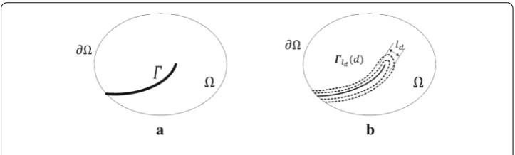
dimensions,∂=∂u∪∂t⊂Rn−1be its boundary andΓ ⊂Rn−1as the sharp crack discontinuity as is schematically depicted in Fig. 2. According to the classical Griffith theory of brittle fracture and assuming small and quasi-static deformations, the total potential may be expressed as the sum of the elastic strain energy, external work and fracture energy given by
ψpot(u,Γ)=
ψe(ε(u))d−
b.ud+
Γ GcdΓ (36)
where ψeis the elastic energy density function of the second order infinitesimal strain tensor,ε(u)= 12∇u+ ∇Tu, andGcis the threshold value of energy releasing from the formation of meso-cracks. The elastic energy density can be written as:
ψe(ε)= 1 2ε:D
e :ε= 1
2λεiiεjj+μεijεij (37)
with the elastic stiffness tensorDeand without loss of generality of Eq. (7), andλandμ as the Lamé constants, which are defined in terms of the elastic (E) and shear (μ) moduli:
λ= νE
(1+ν) (1−2ν), μ≡G= E
Fig. 2 aSharp crack path,Γbapproximated crack path,Γld(d)
The phase field methodology may be regarded as a specific case of non-local gradient model, in which the regularization is performed on sharp crack interfaces with a pure geometrical representation (Fig.2b), as the sharp discontinuity of Fig.2a) is smoothened by an auxiliary phase field variabled∈[0,1], discriminates between the intact (d=0) and fully-broken (d=1) phases. The width of the regularized region is driven by a length scale ld, which may be determined based on the micromechanical observations such as particle shape, size or strength. The sharp discontinuity pattern is recovered for the vanishing length scale. This crack treatment was emerged based on the variational formulation of Francfort and Marigo [21], subsequently complemented by the regularization of Bourdin et al. [22], whereas the classical surface integral of Eq. (36) is replaced by a volume integral, reads the following potential:
ψpot(ε,Γ)=
g(d)ψe(ε(u))d−
b.ud+Gc
Γ
d2 2ld +
ld 2 ∇d
2
dΓ (39)
One commonly used form of the stress degrading functiong(d) is the following mono-tonically decreasing function:
g(d)=(1−d)2+η (40)
whereη 1 is a dimensionless residual stiffness at the total failure to avoid numerical difficulties. This function should satisfy the following properties [25]:
g(0)=1; g(1)=0; g(1)=0 (41)
Based on the work of Miehe et al. [26], the strain tensor can be additively decomposed to the positive (tensile) and negative (compressive) parts in order to avoid cracking under compression:
ε=ε++ε−; ε±= n
a=1
εa±na⊗na (42)
with εa andnaas the eigenvalues and eigenvectors ofεinndimensions, andεa± =
1
2(εa± |εa|).
Accordingly, the degraded isotropic elastic energy function can be decomposed to pos-itive and negative parts:
withψe±(ε)= λ2trε±2+μtrε±2, where the negative part remains undegraded. This leads to the following constitutive law:
σ±=∂εψe(ε, d)=g(d)σ+0 +σ−0 (44)
whereσ±0 =λtr (ε)±+2μεa±na⊗naand∂x(.) is the derivative of function (.) with respect tox. Applying Eqs. (40) and (43) to the potential in Eq. (39), the modified functional may be written as:
ψpot(ε,Γ)=
(1−d)2+η
ψe+(ε)+ψe−(ε)
d−
b.ud +Gc
Γ
d2 2ld +
ld
2 ∇d
2
d (45)
According to the history-field-based formulation in [26], the crack irreversibility condition ( ˙d≤0) is applied to the model at timeton each pointx:
H= max
τ∈[0,t]ψ +
e (ε(x,τ)) (46)
the strong form of the initial boundary value problem can be obtained based on the minimization principles by taking the variation of the functional of Eq. (45),
divσ+b=0 Gc
ld
d−ld2d=2 (1−d)H on (47)
with the following boundary conditions on the displacement field and the phase field:
u=u¯ on∂ u σ.n=tn on∂t
,
d=1 onΓ
∇d.n=0 on∂ (48)
Phase field model in a ductile failure context
Ductile failure occurs in conjunction with extensive plastic deformation. The above phase field approach is applied herein to the plasticity model based on the von Mises hardening criterion. To achieve a thermodynamically-consistent model, the inclusion of the inelastic deformations into the total potential should be considered. This necessitates adding the plastic potential,ψp, to the functional in Eq. (45), which yields the following relation:
ψpot(ε,Γ)=
(1−d)2+η
ψe+(εe)+ψe−(εe)
d−
b.ud +Gc
Γ
d2 2ld +
ld 2 ∇d
2
d∂+
ψp(α)d (49)
This introduces a modified elastoplastic history field:
Hep=βe max
τ∈[0,t]ψ +
e (ε(x,τ))+βpψp(α)−W0 (50)
whereβeandβpare the constants that are regulating the contribution rate of the elastic and plastic works respectively and the Macaulay bracket of an arbitrary variablexis defined as:
x =
x ifx≥0
The second term in Eq. (50) is the part of total energy dissipated by the plastic mechanisms, represented by the following rate form [42,46]:
˙
ψp=γ˙s (52)
whereas the constitutive law expressed in Eq. (44) is adopted. The strong form of Eq. (47)2 may be replaced by the following relation:
Gc ld
d−l2dd=2 (1−d)Hep (53)
Integration algorithm
The integration procedure of this phase field modelling is constructed upon the elas-tic predictor-plaselas-tic corrector algorithm in an analogous way to the presented nonlocal damage model. The calculation of the stress field is carried out based on the von Mises rate-independent plasticity model that may be closely related to the isotropically-hardening plasticity model in [45]. The coupled plasticity model is implemented with UMAT and HETVAL subroutines in Abaqus/Standard (in the same manner that is explained earlier and in “Appendix” for the gradient damage model). In each increment, the phase field value is frozen and retrieved in routine as a temperature field. Given the flux value based on the updated history field from the previous increment in the UMAT code, the updated phase field value is computed through the HETVAL subroutine. This staggered-type solution procedure bypasses the need to calculate the coupled phase-field-displacement tangent terms as is presented in the UEL monotonic scheme in [47].
Havingεand the phase field variable from the previous increment (dn), the predicted elastic trial states are given by:
εe trial
n+1 =εen+ε
ptrialn+1=g(d)Kεe trialv n+1 strial
n+1=2g(d)Gεe triald n+1
¯ εp
n+1=ε¯ p n
¯ σtrial
n+1 =
3J2
strial
n+1
(54)
The yield condition to check the plastic admissiblity is written as:
fy=σ¯ntrial+1 −g(d)σy
¯ εp
n+1
≤0 (55)
If the yield condition is not satisfied, the following return mapping equation is solved iteratively forγ:
¯ σtrial
n+1 −3g(d)Gγ −g(d)σy
¯ εp
n+γ
=0 (56)
By having the solution at hand, the update procedure followed as:
¯ εp
n+1=¯ε
p n+γ
pn+1=g(d)ptrialn+1
sn+1= ¯ σn+1 ¯ σtrial
n+1
σn+1=sn+1+pn+1I εe
n+1= 1
2Gsn+1+ε e trial
v n+1I (57)
The implementation of this algorithm is performed by the same strategy in dealing with the nonlocal gradient damage model discussed before, using steady state heat problem analogy referring to Eq. (34) and assuming the following associations:
κ≡ld2
2ld Gc
(1−d)Hep−d≡q˙
(58)
Results and discussion
The capability of the presented diffusive strategy is assessed herein, through the analysis of two common benchmarks and by observation of force-deflection diagrams, damage evolution, and crack propagation prediction.
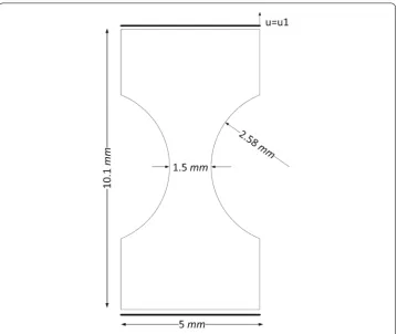
Notched specimen tensile test
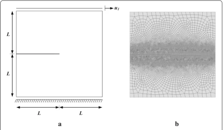
First benchmark is a notched specimen under tension, with the geometry and boundary conditions depicted in Fig.3. This example aims to observe the propagation of the damage and assess the nonlocal gradient damage framework robustness and applicability of the proposed methodology in the post-peak regime to circumvent mesh sensitivity. Due to the symmetry, only one quarter of the specimen is modelled and discretized, assuming distinct mesh discretizations (identically adopted from [48]) and using 4-noded plane strain quadrilateral elements. The material properties used for analysis are represented in Table2, considering that the same length scale is used and treated as a material parameter for all mesh topologies.
Assuming the imposed displacement of u1 = 0.2 mm, the propagation of the local
and non-local damage fields are illustrated in Figs. 4and5 in a same time increment and for three mesh sizes. Expectedly the localization of the damage is at the center of the specimen and, as it proceeds, a 45◦localization band is revealed. The local damage contours show different values by varying the mesh density (denoted byh), whereas the non-local model shows less discrepancy between different meshes at the same chosen time increment. The more sparse damage propagation in non-local case is attributed to the lower values obtained with the non-local model, and it is in a close agreement with the non-local integral-type Lemaitre damage model results presented in [48] (therein stated by L-D).
This can be more plainly observed in the force-deflection diagrams, by comparing the curve discrepancies in Fig.6a, b for the local and non-local damage frameworks respec-tively, where it is visible that mesh sensitivity is attenuated in the case of the non-local model. The results are compared with the results obtained in [48] for local and non-local integral type Lemaitre damage models, showing some discrepancy in the non-local case in which the gradient model predicts less softening than the integral type.
Fig. 3 Geometry and boundary conditions of the notched specimen
Table 2 Material parameters for the notched specimen
Name Value
Young’s modulus (E) 210 GPa
Poisson’s ratio (ν) 0.3
Hardening law σy(α)=700+300 (α)0.3MPa
Lemaitre damage denominator (r1) 3.0 MPa
Lemaitre damage exponent (r2) 1.0
Non-local model length scaleln 0.15 mm
the non-local field with the heat equation solver and therefore the proposed methodology may be utilized with reliability, for this purpose, with this commercial software in the conditions described.
Single edged notched shear test
Fig. 4 Contour plots of the local damage propagation for mesh size ofah=0.25 mm,bh=0.125 mm and
ch=0.094 mm
Fig. 5 Contour plots of the nonlocal damage propagation for mesh size ofah=0.25 mm,bh=0.125 mm andch=0.094 mm
Fig. 6 Force variation with the applied displacement forathe local model andbthe nonlocal model
uses the built-in heat equation solver, by making quantitative comparisons with existing data in literature.
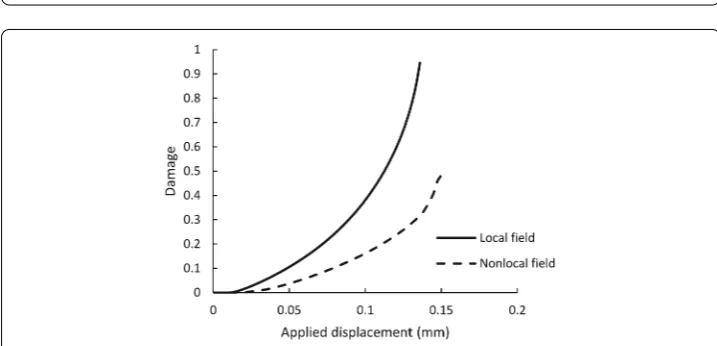
Fig. 7 Evolution of damage field at the central node fromathe local model andbthe non-local model
Fig. 8 Evolution of damage fields at the central node obtained from the refined mesh
from the undamaged zones. The material properties, mainly, taken from reference [37], are summarized in Table3while the same contribution rates of elastic and plastic works are considered herein,βe=βp=1.0.
Fig. 9 Single edge notched testageometry and boundary conditionsbmesh discretization
Table 3 Material parameters for the single edge notched test
Name Value
Young’s modulus (E) 180 GPa
Poisson’s ratio (ν) 0.28
Yield stress (σy) 443 MPa
Hardening modulus 300 MPa
Phase field model length scaleld 0.06
Critical energy release rate (Gc) 15 N/mm
Residual stiffness 1.0e−5
βeandβp 1.0
Plastic work threshold (W0) 1.0
Fig. 10 Contour plots of equivalent plastic straina(1–3) and the regularized crackb(1–3) atu1=0.1 mm,
Fig. 11 Mesh sensitivity of the proposed phase field model and comparison with the results in [37]
Concluding remarks
In this study, the evolution of damage and failure, via non-local gradient damage and phase field models, respectively, was simulated resorting to an analogy to heat diffusion in solids, using the built-in thermo-mechanically coupled finite-element solution procedure in Abaqus. The developed procedure was justified and assessed in terms of qualitative verification of crack propagation patterns and its capability of avoiding mesh dependence pathologies.
The utilization of this approach may be viewed as a simple alternative to include the regu-larization procedures associated with both gradient and phase field models in commercial codes with no need of cumbersome implementations of explicit weak form derivations within required lengthy user files.
Authors’ contributions
All authors contributed in the material modelling and simulation procedure of the article. EA carried out the user coding of the damage model and phase field method as well as the benchmark testing of the single edge notched test, and drafted the manuscript. JPSF contributed in the utilization of the heat equation solver of Abaqus in modelling the gradient regularization, and performed the numerical assessment on the notched specimen tensile test with the respective gradient damage model. JCS and MPLP supervised the study and did the corrections on the manuscript draft. All authors read and approved the final manuscript.
Acknowledgements
Authors gratefully acknowledge the funding of Project NORTE-01-0145-FEDER-000022—SciTech—Science and Technology for Competitive and Sustainable Industries, cofinanced by Programa Operacional Regional do Norte (NORTE2020), through Fundo Europeu de Desenvolvimento Regional (FEDER) and the project Grant
SFRH/BD/107860/2015 of the Portuguese foundation of science.
Competing interests
The authors declare that they have no competing interests.
Availability of data and materials Not applicable.
Consent for publication Not applicable.
Ethics approval and consent to participate Not applicable.
Appendix
!---! User material ABAQUS coupled temperature-displacement problems. ! Temperature field is treated as nonlocal damage field.
!---! Following keywords must be defined at INP file
! *Element, type=***T, ...
! *Initial Conditions, type=TEMPERATURE ! *HEAT GENERATION
! *Depvar
! *Coupled Temperature-displacement ! 0.01, 100., 1e-06, 1.0
! <inc_intial>, <total time>, <inc_min>, <inc_max>
!---! Subroutine HETVAL:
! Gradient damage equation: D-D_BAR=L_N^^2*GRAD2(D_BAR) ! STATEV(6) : Local damage variable
! STATEV(7) : Nonlocal damage variable (TEMP)
!---SUBROUTINE HETVAL(CMNAME,TEMP,TIME,DTIME,STATEV,FLUX, 1 PREDEF,DPRED)
!
INCLUDE 'ABA_PARAM.INC' !
CHARACTER*80 CMNAME !
DIMENSION TEMP(2),STATEV(*),PREDEF(*),TIME(2),FLUX(2), 1 DPRED(*)
!---! HEAT FLUX = LOCAL DMG – NONLOCAL DMG
FLUX(1)=STATEV(6)-STATEV(7) FLUX(2)=ZERO
!---RETURN END
!---! Subroutine UMAT
! User coding to treat displacement field, update stresses, ! strains and damage fields
! STATEV(1-4): Elastic strains
! STATEV(5): Equivalent plastic strain ! STATEV(6): Local damage variable
! STATEV(7): Nonlocal damage variable(TEMP)
!---SUBROUTINE UMAT(STRESS, STATEV, DDSDDE, SSE, SPD, SCD, RPL, 1 DDSDDT, DRPLDE, DRPLDT, STRAN, DSTRAN, TIME, DTIME, TEMP, DTEMP, 2 PREDEF, DPRED, CMNAME, NDI, NSHR, NTENS, NSTATV, PROPS, NPROPS, 3 COORDS, DROT, PNEWDT, CELENT, DFGRD0, DFGRD1, NOEL, NPT, LAYER, 4 KSPT, KSTEP, KINC)
INCLUDE 'ABA_PARAM.INC' !
CHARACTER*8 CMNAME !
! Argument lists and routine inputs … !
MU=EMOD/(TWO*(ONE+ENU)) TWOMU=TWO*MU
THREEMU=OP5*TWOMU SIXMU=SIX*MU
ALAMBDA=TWOMU*ENU/(ONE-TWO*ENU) E3BULK=EMOD/(ONE-TWO*ENU) EBULK=E3BULK*THIRD
E2BULK=TWO*EBULK
!---! Initialization of the tangent matrix
!
DO K1=1, NDI
DO K2=1, NDI
DDSDDE(K2, K1)=ALAMBDA
END DO
DDSDDE(K1, K1)=TWOMU+ALAMBDA
END DO
DO K1=NDI+1,NTENS DDSDDE(K1, K1)=MU
END DO
!---! Recover elastic strains, plastic strain,
! equivalent plastic strain and damage variable !
DO K1=1,NTENS
EELAS(K1)=STATEV(K1)
ENDDO
EQPLASN=STATEV(5) DAMAGEN=STATEV(6) DAMAGENL=STATEV(7) OMEGAN=ONE-DAMAGEN OMEGANL=ONE-DAMAGENL
!---! Elastic Step
!
DO K1=1,NTENS
DO K2=1,NTENS
STRESS(K2)=STRESS(K2)+OMEGAN*DDSDDE(K2,K1)*DSTRAN(K1)
ENDDO
EELAS(K1)=EELAS(K1)+DSTRAN(K1)
ENDDO
!---! User coding to define volumetric and deviatoric strain
! components, equivalent stress and the current yield stress :
:
QTRIAL=SQRT(THREE*J2T)/OMEGAN ! local model equivalent stress QTRIALNL=SQRT(THREE*J2T)/OMEGANL ! Nonlocal model equivalent stress ! Call to the hardening routine to obtain yield stress
! and hardening data !
!---! Calculate the yield function and check for plastic admissibility !
FYIELD=QTRIAL-SYIEL0 !
IF (FYIELD.GT.TOLER*SYIEL0) THEN
!---! Begin the return mapping algorithm based on Lemaitre ductile
! damage model simplified version as presented by de Souza Neto et al. !
!
! Initialization of variables :
DGAMMA=OMEGAN*FYIELD/THREEMU EQPLAS=EQPLASN+DGAMMA
!---! Start Newton Iterations
!---DO 50 IITER=1,NITER
! Call to the hardening routine yield2=SYIELD*SYIELD
!
! Initialize OMEGA and some other variables :
: !
! Damage Energy Release Rate
Y=(-yield2/SIXMU)-PTRIA2/E2BULK
RES=OMEGA-OMEGAN+DGAMMA/OMEGA*(-Y/DAMDEN)**DAMEXP
!---! Convergence check
!---IF (ABS(RES).LE.TOLER) THEN
!---! NR Convergence verified
!---! Update the local damage field
DAMAGE=ONE-OMEGA
!---! Nonlocal damage of the previous converged increment is used ! to stablish current STRESS and DDSDDE
!---OMEGA=ONE-DAMAGENL
!
IF (DAMAGE.GT.ONE) THEN
DAMAGE=DAMAGEN ENDIF
IF (DAMAGENL.GT.ONE) CALL XIT
!
P=OMEGA*PTRIAL Q=OMEGA*SYIELD
FACTOR=TWOMU*Q/QTRIALNL !
! Update strains
FACTOR2=ONE-THREEMU*DGAMMA/(OMEGA*QTRIAL) STATEV(1)=FACTOR2*EED(1)+EEVD3
STATEV(2)=FACTOR2*EED(2)+EEVD3 STATEV(3)=FACTOR2*EED(3)+EEVD3 STATEV(4)=FACTOR2*EED(4)*TWO !
! Update stresses
DO K1=1,NDI
STRESS(K1)=FACTOR*EED(K1)+P ENDDO
DO K1=NDI+1,NTENS
STRESS(K1)=FACTOR*EED(K1) ENDDO
!
!---! UPDATE INTERNAL VARIABLES
NONLOCAL VARIABLE VALUE IS THE CURRENT ‘TEMPERATURE’ VALUE
!---! Call to a routine to calculate the Lemaitre damage consistent tangent operator !
: :
ENDIF
! User coding to define the derivatives :
:
!---! End loop over Newton iterations
50 CONTINUE
!---! Newton-Raphson Convergence Error
WRITE(7,*) '*ERROR* THE N-R ALGORITHM FAILED TO BE CONVERGED AFTER'
1 IITER,'ITERATIONS'
CALL XIT
!---ELSE
!---! Elastic step
!---FACTOR0=TWOMU*OMEGAN
P=OMEGAN*PTRIAL
DO K1=1,NDI
STRESS(K1)= FACTOR0*EED(K1)+P ENDDO
DO K1=NDI+1,NTENS
STRESS(K1)= FACTOR0*EED(K1) ENDDO
ENDIF !
DO K1=1,NTENS
STATEV(K1)=EELAS(K1) ENDDO
!---! UPDATE INTERNAL VARIABLES
NONLOCAL VARIABLE VALUE IS THE CURRENT ‘TEMPERATURE’ VALUE
!---STATEV(5)=EQPLAS STATEV(6)=DAMAGE STATEV(7)=TEMP
!---!
RETURN END
Publisher’s Note
Springer Nature remains neutral with regard to jurisdictional claims in published maps and institutional affiliations.
Received: 14 December 2017 Accepted: 24 April 2018
References
1. Lemaitre J. A continuous damage mechanics model for ductile fracture. J Eng Mater Technol. 1985;107:83–9.https:// doi.org/10.1115/1.3225775.
2. Bourdin B, Francfort GA, Marigo JJ. The variational approach to fracture. J Elast. 2008;91(1–3):5–148.
3. Rice JR, Tracey DM. On the ductile enlargement of voids in triaxial stress fields*. J Mech Phys Solids. 1969;17:201–17. https://doi.org/10.1016/0022-5096(69)90033-7.
4. Gurson AL. Continuum theory of ductile rupture by void nucleation and growth: part I-yield criteria and flow rules for porous ductile media. J Eng Mater Technol. 1977;99:2.https://doi.org/10.1115/1.3443401.
5. Tvergaard V, Needleman A. Analysis of the cup-cone fracture in a round tensile bar. Acta Metall. 1984;32:157–69. https://doi.org/10.1016/0001-6160(84)90213-X.
6. Kachanov L. Time of the rupture process under creep condition. Izv Akad Nauk SSSR Otd Tekhn Nauk. 1958;8:26–31. 7. Lemaitre J. A continuous damage mechanics model for ductile fracture. J Eng Mater Technol. 1985;107:83.https://
doi.org/10.1115/1.3225775.
8. Chaboche JL. Continuum damage mechanics: part 1—general concepts. J Appl Mech. 1988;55:59.
10. Benallal A, Billardon R, Doghri I. An integration algorithm and the corresponding consistent tangent operator for fully coupled elastoplastic and damage equations. Commun Appl Numer Methods. 1988;4:731–40.https://doi.org/ 10.1002/cnm.1630040606.
11. de Souza Neto EA, Peri´c D, Owen DRJ. Continuum modelling and numerical simulation of material damage at finite strains. Arch Comput Methods Eng. 1998;5:311–84.https://doi.org/10.1007/BF02905910.
12. Pijaudier-Cabot G, Bažant ZP. Nonlocal damage theory. J Eng Mech. 1987;113(10):1512.https://doi.org/10.1061/ (ASCE)0733-9399.
13. Peerlings RHJ, De Borst R, Brekelmans WAM, de Vree JHP. Gradient enhanced damage for quasi-brittle materials. Int J Numer Methods Eng. 1996;39:3391–403.https://doi.org/10.1002/(SICI)1097-0207(19961015)39:19<3391:: AID-NME7>3.0.CO;2-D.
14. De Borst R, Pamin J, Geers MGD. On coupled gradient-dependent plasticity and damage theories with a view to localization analysis. Eur J Mech A/Solids. 1999;18:939–62.https://doi.org/10.1016/S0997-7538(99)00114-X. 15. Comi C. Computational modelling of gradient-enhanced damage in quasi-brittle materials. Mech
Cohesive-Frictional Mater. 1999;4:17–36.https://doi.org/10.1002/(SICI)1099-1484(199901)4:1<17::AID-CFM55>3.0. CO;2-6.
16. Engelen RAB, Geers MGD, Baaijens FPT. Nonlocal implicit gradient-enhanced elasto-plasticity for the modelling of softening behaviour. Int J Plast. 2002;19:403–33.https://doi.org/10.1016/S0749-6419(01)00042-0.
17. Geers MGD, Ubachs RLJM, Engelen RAB. Strongly non-local gradient-enhanced finite strain elastoplasticity. Int J Numer Methods Eng. 2003;56:2039–68.https://doi.org/10.1002/nme.654.
18. Areias PMA, de Sá JC, António CC. A gradient model for finite strain elastoplasticity coupled with damage. Finite Elem Anal Des. 2003;39:1191–235.https://doi.org/10.1016/S0168-874X(02)00164-6.
19. Almansba M. Isotropic elastoplasticity fully coupled with non-local damage. Engineering. 2010;2:420–31.https://doi. org/10.4236/eng.2010.26055.
20. Javani HR, Peerlings RHJ, Geers MGD. Consistent remeshing and transfer for a three dimensional enriched mixed formulation of plasticity and non-local damage. Comput Mech. 2014;53:625–39.https://doi.org/10.1007/ s00466-013-0922-z.
21. Francfort GA, Marigo JJ. Revisiting brittle fracture as an energy minimization problem. J Mech Phys Solids. 1998;46:1319–42.https://doi.org/10.1016/S0022-5096(98)00034-9.
22. Bourdin B, Francfort GA, Marigo JJ. Numerical experiments in revisited brittle fracture. J Mech Phys Solids. 2000;48:797–826.https://doi.org/10.1016/S0022-5096(99)00028-9.
23. Mumford D, Shah J. Optimal approximations by piecewise smooth functions and associated variational problems. Commun Pure Appl Math. 1989;42:577–685.https://doi.org/10.1002/cpa.3160420503.
24. Karma A, Kessler DA, Levine H. Phase-field model of mode III dynamic fracture. Phys Rev Lett. 2001;87(4):045501. https://doi.org/10.1103/PhysRevLett.87.045501.
25. Miehe C, Welschinger F, Hofacker M. Thermodynamically-consistent phase field models of fracture: variational principles and multi-field FE implementations. J Numer Methods Eng. 2009;83(10):1273–311.
26. Miehe C, Hofacker M, Welschinger F. A phase field model for rate-independent crack propagation: robust algorithmic implementation based on operator splits. Comput Methods Appl Mech Eng. 2010;199:2765–78.https:// doi.org/10.1016/j.cma.2010.04.011.
27. Kuhn C, Müller R. A continuum phase field model for fracture. Eng Fract Mech. 2010;77:3625–34.https://doi.org/10. 1016/j.engfracmech.2010.08.009.
28. Pham K, Amor H, Marigo JJ, Maurini C. Gradient damage models and their use to approximate brittle fracture. Int J Damage Mech. 2011;20:618–52.https://doi.org/10.1177/1056789510386852.
29. Borden MJ, Verhoosel CV, Scott MA, et al. A phase-field description of dynamic brittle fracture. Comput Methods Appl Mech Eng. 2012;217–220:77–95.https://doi.org/10.1016/j.cma.2012.01.008.
30. Borden MJ, Hughes TJR, Landis CM, Verhoosel CV. A higher-order phase-field model for brittle fracture: formulation and analysis within the isogeometric analysis framework. Comput Methods Appl Mech Eng. 2014;273:100–18. https://doi.org/10.1016/j.cma.2014.01.016.
31. Ambati M, Gerasimov T, De Lorenzis L. A review on phase-field models of brittle fracture and a new fast hybrid formulation. Comput Mech. 2014;55:383–405.https://doi.org/10.1007/s00466-014-1109-y.
32. Verhoosel CV, de Borst R. A phase-field model for cohesive fracture. Int J Numer Methods Eng. 2013;96:43–62. https://doi.org/10.1002/nme.4553.
33. Nguyen TT, Yvonnet J, Zhu QZ, et al. A phase field method to simulate crack nucleation and propagation in strongly heterogeneous materials from direct imaging of their microstructure. Eng Fract Mech. 2015;139:18–39.https://doi. org/10.1016/j.engfracmech.2015.03.045.
34. Guo XH, Shi SQ, Ma XQ. Elastoplastic phase field model for microstructure evolution. Appl Phys Lett. 2005;87:1–3. https://doi.org/10.1063/1.2138358.
35. Voyiadjis GZ, Mozaffari N. Nonlocal damage model using the phase field method: theory and applications. Int J Solids Struct. 2013;50:3136–51.https://doi.org/10.1016/j.ijsolstr.2013.05.015.
36. Duda FP, Ciarbonetti A, Sánchez PJ, Huespe AE. A phase-field/gradient damage model for brittle fracture in elastic-plastic solids. Int J Plast. 2014;65:269–96.https://doi.org/10.1016/j.ijplas.2014.09.005.
37. Ambati M, Gerasimov T, De Lorenzis L. Phase-field modeling of ductile fracture. Comput Mech. 2015;55:1017–40. https://doi.org/10.1007/s00466-015-1151-4.
38. Hernandez Padilla CA, Markert B. A coupled phase-field model for ductile fracture in crystal plasticity. PAMM. 2014;14:441–2.https://doi.org/10.1002/pamm.201410208.
39. Mozaffari N, Voyiadjis GZ. Phase field based nonlocal anisotropic damage mechanics model. Phys D Nonlinear Phenom. 2015;308:11–25.https://doi.org/10.1016/j.physd.2015.06.003.
41. Miehe C, Hofacker M, Schaenzel LMM, Aldakheel F. Phase field modeling of fracture in multi-physics problems. Part II. Coupled brittle-to-ductile failure criteria and crack propagation in thermo-elastic-plastic solids. Comput Methods Appl Mech Eng. 2015;294:1–37.https://doi.org/10.1016/j.cma.2014.11.017.
42. Badnava H, Etemadi E, Msekh M. A phase field model for rate-dependent ductile fracture. Metals (Basel). 2017;7:180. https://doi.org/10.3390/met7050180.
43. de Borst R, Verhoosel CV. Gradient damage vs phase-field approaches for fracture: similarities and differences. Comput Methods Appl Mech Eng. 2016;312:78–94.https://doi.org/10.1016/j.cma.2016.05.015.
44. Geers MGD, de Borst R, Brekelmans WAM, Peerlings RHJ. Strain-based transient-gradient damage model for failure analyses. Comput Methods Appl Mech Eng. 1998;160:133–53.https://doi.org/10.1016/S0045-7825(98)80011-X. 45. de Souza Neto EA, Peric D, Owen RJ. Computational methods for plasticity. New York: Wiley; 2008.
46. Borden MJ, Hughes TJR, Landis CM, et al. A phase-field formulation for fracture in ductile materials: finite deformation balance law derivation, plastic degradation, and stress triaxiality effects. Comput Methods Appl Mech Eng. 2016;312:130–66.https://doi.org/10.1016/j.cma.2016.09.005.
47. Msekh MA, Sargado JM, Jamshidian M, et al. Abaqus implementation of phase-field model for brittle fracture. Comput Mater Sci. 2015;96:472–84.https://doi.org/10.1016/j.commatsci.2014.05.071.

![Fig. 11 Mesh sensitivity of the proposed phase field model and comparison with the results in [37]](https://thumb-us.123doks.com/thumbv2/123dok_us/9580143.1940834/18.595.117.478.84.248/mesh-sensitivity-proposed-phase-eld-model-comparison-results.webp)
