The Thirty-Third AAAI Conference on Artificial Intelligence (AAAI-19)
Bi-Kronecker Functional Decision Diagrams:
A Novel Canonical Representation of Boolean Functions
Xuanxiang Huang, Kehang Fang, Liangda Fang,
*Qingliang Chen, Zhao-Rong Lai, Linfeng Wei
Department of Computer Science, Jinan UniversityGuangzhou 510632, China
[email protected]; [email protected];{fangld,tpchen,laizhr,twei}@jnu.edu.cn
Abstract
In this paper, we present a novel data structure for compact representation and effective manipulations of Boolean func-tions, called Bi-Kronecker Functional Decision Diagrams (BKFDDs). BKFDDs integrate the classical expansions (the Shannon and Davio expansions) and their bi-versions. Thus, BKFDDs are the generalizations of existing decision dia-grams: BDDs, FDDs, KFDDs and BBDDs. Interestingly, un-der certain conditions, it is sufficient to consiun-der the above ex-pansions (the classical exex-pansions and their bi-versions). By imposing reduction and ordering rules, BKFDDs are compact and canonical forms of Boolean functions. The experimental results demonstrate that BKFDDs outperform other existing decision diagrams in terms of sizes.
Introduction
A representation of Boolean functions, which has a com-pact size and supports effective manipulations, plays a dom-inant role in the area of artificial intelligence,e.g., planning (Palacios et al. 2005; Huang 2006), diagnosis (Huang and Darwiche 2005; Siddiqi and Huang 2007), and probabilis-tic inference (Chavira and Darwiche 2008; Fierens et al. 2015). The most notable representation isBinary Decision Diagrams (BDDs)(Bryant 1986) that are based onthe Shan-non expansion(Boole 1854; Shannon 1938). The Shannon expansion splits a function into two cofactors w.r.t. the vari-ablexand its complement x¯. Moreover,the (positive and negative) Davio expansions1 are more suitable to serve as the basis of decomposing XOR-intensive functions than the Shannon one (Kebschull, Schubert, and Rosenstiel 1992). Based on the Davio expansion, Functional Decision Dia-grams (FDDs) are proposed in (Kebschull, Schubert, and Rosenstiel 1992; 1993; Drechsler, Theobald, and Becker 1996). However, it is shown that either of BDDs or FDDs alone is inefficient for representing some classes of Boolean functions (Becker and Drechsler 1995b). To address this deficit, Drechsler and Becker (1998) proposed Kronecker Functional Decision Diagrams (KFDDs)that integrate the
*Corresponding author
Copyright © 2019, Association for the Advancement of Artificial Intelligence (www.aaai.org). All rights reserved.
1
The Davio expansion is also called the Reed-Muller expansion (Reed 1954; Muller 1954).
aforementioned three expansions. In both theory and prac-tices, KFDDs turns out to be more compact than BDDs and FDDs.
The notion of expansions is the theoretical foundation of decision diagrams. A generalization to the Shannon expan-sion (Kerntopf 2001) has been proposed for a long time. This generalization decomposes a function into two cofac-tors w.r.t. an auxiliary functiongand its negationg¯. How-ever, identifying a suitable auxiliary function for the gener-alized Shannon expansion is hard, which hinders it serving as the core theory of decision diagrams that enjoys effec-tive operations. Recently, a simple fragment, calledthe bi-Shannon expansion, restricting the auxiliary function to be a single variable, has been proposed in (Amar´u, Gaillardon, and Micheli 2014). Based on the above expansion, Bicon-ditional Binary Decision Diagrams (BBDDs)are developed accordingly. Thanks to the simplicity of the bi-Shannon ex-pansion, Boolean manipulations on BBDDs are efficient.
It can be observed that (1) the more expansions the deci-sion diagram is empowered by, the more compact it is, and (2) the simpler expansions the decision diagram uses, the more effective it is. In this paper, we thus aim to design a decision diagram that fuses as many expansions as possible under the principle of adopting simple ones.
The main contributions of this paper are as follows:
1. Inspired by the idea of the bi-Shannon expansion, we propose two invariants of Davio expansion, called the bi-positive and bi-negative Davio expansions.
2. By combining the above two expansions together with the existing ones (Shannon, bi-Shannon, and positive and negative Davio), we develop a novel representa-tion of Boolean funcrepresenta-tions, called bi-Kronecker Func-tional Decision Diagrams (BKFDDs). Due to the diver-sity of the expansions, BKFDDs are generalizations of the existing decision diagrams: BDDs, FDDs, KFDDs and BBDDs. Interestingly, we show that, under certain conditions, only some essential expansions are neces-sary,i.e., the other ones can indeed be reduced to one of them.
compresses chain structures in decision diagrams into single nodes.
4. We also introduce the algorithms for Boolean manipula-tions on BKFDDs, and analyze their complexities. 5. Experiments are carried out to compare BDDs, KFDDs,
BBDDs and BKFDDs on the MCNC benchmarks2. The empirical results show that BKFDDs outperform other decision diagrams in terms of sizes.
Preliminaries
In this section, we briefly review some background knowl-edge on decision diagrams.
Throughout this paper, we fix a set Xwith nvariables
x1,· · ·, xn. We say a Boolean functionf : Bn → B is
simple, if it is a Boolean constant0or1, a variablexi or
its negationx¯i. It is well-known that any Boolean function f : Bn → Bcan be represented by BDDs (Bryant 1986).
A BDD is a rooted directed acyclic graph with two types of nodes: internal and terminal nodes. Each terminal node denotes a constant1or0. Each internal node, labeled with a variablexi, represents a function according to the Shannon
expansion:
f = ¯xi·fxi=0+xi·fxi=1(S)
wherefxi=0 (resp.fxi=1) is the function obtained fromf
by replacingxiwith0(resp.1).
A Boolean function has many different BDD representa-tions. To ensure the canonicity of BDDs,i.e., every function has a unique BDD, two constraints are imposed on BDDs (Bryant 1986). Given a variable orderπ, a BDD isordered, if each variable appears at most once on each path from the root to a terminal node, and the variables appear following the orderπon all such paths. A BDD isreduced, if it con-tains neither isomorphic subgraphs nor nodes with isomor-phic children. Ordered and reduced BDDs are canonical rep-resentations for Boolean functions.
The Davio expansion defined below (Kebschull, Schu-bert, and Rosenstiel 1992) is more suitable for XOR-intensive Boolean functions than the Shannon one.
f =fxi=0⊕xi·(fxi=0⊕fxi=1)(pD)
f =fxi=1⊕x¯i·(fxi=0⊕fxi=1)(nD)
Based on the positive Davio expansion, a variant of BDDs, called FDDs, is proposed in (Kebschull, Schubert, and Rosenstiel 1992; 1993). As before, by imposing reduction and ordering rules, FDDs are canonical.
For certain classes of Boolean functions, their BDD rep-resentations are exponentially larger than their FDD ones, and vice versa (Becker and Drechsler 1995b). Drechsler and Becker (1998) proposed KFDDs that combines the above three expansions. With both characteristics of BDDs and FDDs, KFDDs are more compact and general representa-tions for Boolean funcrepresenta-tions.
Later on, it was shown that the Shannon and Davio expan-sions can be generalized as follows (Kerntopf 2001):
f = (¯xi⊕g)·fxi=g+ (xi⊕g)·fxi=¯g(gS)
2
https://ddd.fit.cvut.cz/prj/Benchmarks/
f =fxi=g⊕(xi⊕g)·(fxi=g⊕fxi=¯g)(gpD)
f =fxi=¯g⊕(¯xi⊕g)·(fxi=g⊕fxi=¯g)(gnD)
It is obvious that the generalized Shannon expansion degen-erates into the classical one if g is substituted by 0. Nev-ertheless, finding a proper auxiliary Boolean function g is a hard problem. Recently, Amar´u, Gaillardon, and Micheli (2014) considered the simple case where the auxiliary func-tion is a single variable xj, and proposed the bi-Shannon
expansion:
f = (¯xi⊕xj)·fxi=xj + (xi⊕xj)·fxi=¯xj (bS)
Based on this expansion, Amar´u, Gaillardon, and Micheli (2014) developed BBDDs, and showed that BBDDs are more compact than BDDs for two famous Boolean func-tions: Majority and Adder.
Bi-Kronecker Functional Decision Diagrams
In this section, we introduce a novel decision diagram, calledBi-Kronecker Functional Decision Diagram (BKFDD). We first extend both positive and negative Davio expansions to their variants, namely positive Davio (bpD) and bi-negative Davio (bnD). By integrating the six expansions: S, pD, nD, bS, bpD and bnD, we obtain the BKFDDs that are the generalizations of the existing decision diagrams: BDDs, FDDs, KFDDs, and BBDDs. Then, we show that BKFDDs are canonical under the ordering and reduction rules. Interestingly, with the help of complemented edges, it is found that the above six expansions are different only when the auxiliary function is simple. Finally, the algorithms for Boolean operations on BKFDDs are given.
The structure
Inspired by the bi-Shannon expansion, we naturally provide the bi-version of Davio expansions as follows:
f =fxi=xj ⊕(xi⊕xj)·(fxi=xj⊕fxi=¯xj)(bpD)
f =fxi=¯xj ⊕(¯xi⊕xj)·(fxi=xj⊕fxi=¯xj)(bnD)
For better illustration, we classify the six expansions (S, pD, nD, bS, bpD and bnD) into two groups. The first three expansions are calledclassical expansionswhile the latter three ones are calledbi-expansions.
We hereafter introduce BKFDD that integrates the above six expansions. The formal definition of decision diagrams, which serves as the basis of BKFDD, is given as follows.
Definition 1. Adecision diagram (DD) is a rooted directed acyclic graph consisting of two types of nodes: internal and terminal nodes. Each internal nodevis labeled with a pair (xi, g)wherexi ∈Xandgis a Boolean function, and has
two successors:low(v)andhigh(v). Each terminal nodevis labeled with a constant1or0and has no successor.
only the decision variable but also the auxiliary function. As mentioned before, it is difficult to identify a suitable auxil-iary function for internal nodes. In this paper, the choice of auxiliary functions is relatively easy since we only consider the classical expansions and bi-expansions. Hence, the aux-iliary functiongis either a Boolean constant0or a distinct variablexj(i.e.,i6=j). We remark that it is not necessary to
consider the cases wheregis1orx¯j as they are redundant
which will be explained later.
Just as BDDs and FDDs are characterized by a variable order, BKFDDs are characterized by a variable order aug-mented with expansion types (OET).
Definition 2. Avariable order with expansion types (OET)
π is a sequence of npairs (x, e) wherex ∈ X ande ∈ {S, pD, nD, bS, bpD, bnD} such that the variables of any two distinct pairs are different.
For a pair (x, e), x is called the variable of the pair, and e is called the expansion type. For an OET π, we use πx for the variable order following π, π
i for the i
-th element of π, πx
i for the variable of πi, and πei for
the expansion type of πi. For example, suppose that π
is an OET [(x2, pD),(x3, bS),(x1, bnD),(x4, bS)].
Fol-lowing the OET π, we get that πx is a variable order
[x2, x3, x1, x4],π3= (x1, bnD),π3x=x1, andπ3e=bnD.
To determine the Boolean function to which a DD corre-sponds, it is necessary to identify the auxiliary function and expansion type of each internal node. To achieve this, we present therespecting relationbetween DDs and OETs.
Definition 3. We say a DD Grespects an OET π, if the following conditions hold for each internal nodev labeled with(πxi, g),
1. g=0whenπe
i ∈ {S, pD, nD}ori=n;
2. g=πx
i+1whenπie∈ {bS, bpD, bnD}andi6=n.
For an arbitrary internal nodevwhose decision variable isπx
i, ifvis associated with one of the classical expansions,
then its auxiliary function is0. If the expansion type ofv
is a bi-expansion, andi < n, then its auxiliary function is
πxi+1. We note that if the decision variable ofv is the last element ofπx, then the node associated with a bi-expansion
degenerates into a node associated with the corresponding classical expansion, and thus its auxiliary function becomes 0.
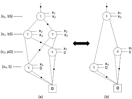
Example 1. An OETπ: [(x1, bS),(x2, bS),(x3, pD),(x4,
S)] is given in Figure 1. Thus, πx = [x1, x2, x3, x4] and
π1= (x1, bS). In Figure 1(a), the decision variable of node
1isx1. It follows that the auxiliary function of node1is the
variablex2. Similarly, the auxiliary function of node4is0.
We say a DDGrespecting an OETπis a BKFDDGπ.
Then we are ready to give the correspondence between BKFDDs and Boolean functions.
Definition 4. LetGbe a BKFDD respecting an OETπ. The Boolean functionfG :Bn →Brepresented byGis defined
as follows.
1. IfGconsists of only one terminal node labeled with1 (resp.0), thenfG=1(resp.0).
Figure 1: Graphical depiction of the weak ROBKFDD (a) and strong ROBKFDD (b) for the functionf = ¯x1·x3+
(¯x1⊕x3)·x¯4. The dashed line denotes the low-edge and the
solid line denotes the high-edge. The dotted line denotes the complemented edge.
2. If G is associated with the root node v labeled with (x, g), then
fG=
(¯x⊕g)flow(v)+ (x⊕g)fhigh(v) ife∈ {S, bS}
flow(v)⊕(x⊕g)fhigh(v) ife∈ {pD, bpD}
flow(v)⊕(¯x⊕g)fhigh(v) ife∈ {nD, bnD}
where(x, e) ∈ π,flow(v) andfhigh(v)are the Boolean
functions represented by the BKFDD rooted bylow(v) andhigh(v), respectively.
We hereafter introduce the ordering rule for BKFDDs.
Definition 5. Given an OETπ, we say a BKFDD is an or-deredBKFDD (OBKFDD), if for each path from the root to a terminal node, we have
1. For any two distinct internal nodes on the path, their de-cision variables are different.
2. The decision variables of internal nodes on such path appear followingπx.
3. For any internal node v on the path, if its auxiliary function is a variableπx
i and its successors are internal
nodes, then the decision variables of successors ofvis
πx
j wherej≥i.
We remark that the constant0is considered as a variable that is the last one following any OET, since auxiliary func-tions of some nodes of bi-expansion types are0.
For example, in Figure 1(a), three internal nodes labeled with1,2 and5are in a path from the root node to the ter-minal node 0. The decision variables of them are x1, x2
and x4 respectively. It is easy to observe that their
deci-sion variables are different, and appear following the order
πx : [x
1, x2, x3, x4]. In addition, the auxiliary functions of
node1isx2, and node2is a successor of node1. Thus, the
decision variable of node2isx2.
A node labeled with (πxi, g)in a BKFDD Gπ is called
aπe
i-node. For example, a node in a BKFDD is called an
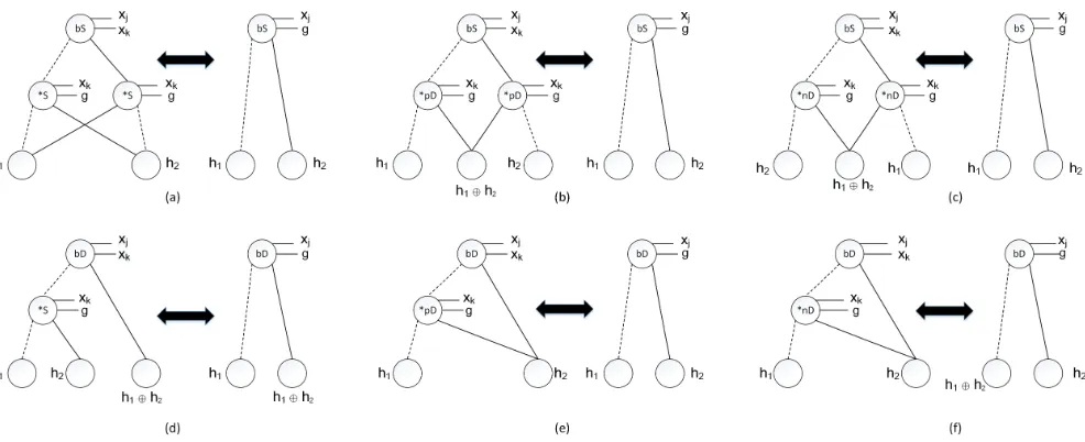
Figure 2: The ruleRCwhere a node labeled with “*S” is an S- or bS-node, a node labeled with “bD” is a bpD- or bnD-node, a node labeled with “*pD” is a pD- or bpD-node, and a node labeled with “*nD” means this node is a nD- or bnD-node.
node5in Figure 1(a) is an S-node. Furthermore, it is easily verified that BKFDDs are generalizations of the four DDs: BDDs, FDDs, KFDDs, and BBDDs. For example, BKFDDs degenerates into KFDDs by only considering classical ex-pansions.
Reduction rules and canonicity
In order to compactly represent Boolean functions, BKFDDs should be compressed to another one denoting the same function according to a set of reduction rules. In the following, we propose reduction rules for BKFDDs that are inherited from KFDDs (Drechsler and Becker 1998), and obtain the canonicity theorem for OBKFDDs.
RI Eliminate a nodevisomorphic to a distinct nodev0, and redirect all incoming edges ofvtov0.
RS Eliminate a nodev whose two successors arev0, and redirect all incoming edges ofvtov0.
RD Eliminate a node v such that the successor high(v) points to the terminal node0, and redirect all incom-ing edges ofvtolow(v).
The rule RIcan be applied in any node of OBKFDDs. However, the rule RS is applied only in S- and bS-nodes while the rule RD is applied only in pD-, nD-, bpD-and bnD-nodes. We say an OBKFDD is a weak reduced
OBKFDD (weak ROBKFDD), if none of the rulesRI,RS andRDcan be applied in it.
By repeated applications of the above three rules, we ob-tain a canonical representation for Boolean functions.
Theorem 1. For any Boolean functionf and OETπ, there is exactly one weak ROBKFDD such that it respectsπand representsf.
Thanks to the simplicity of auxiliary functions and bi-expansions, BKFDDs can be further compressed by new re-duction rules. Let us illustrate it in the following example.
Example 2. Letf = ¯x1·x3+ (¯x1⊕x3)·x¯4. Figure 1(a)
depicts a weak ROBKFDD D representing the functionf
with6 nodes. Interestingly, the nodes on the second level can be eliminated according to the following equation:
f= (¯x1⊕x3)·¯x4+ (x1⊕x3)·x3
= [(¯x1⊕x2)⊕(x2⊕x3)]·x¯4+ [(x1⊕x2)⊕(x2⊕x3)]·x3 = (¯x1⊕x2)·(¯x2⊕x3)·¯x4+ (¯x1⊕x2)·(x2⊕x3)·x3+
(x1⊕x2)·(¯x2⊕x3)·x3+ (x1⊕x2)·(x2⊕x3)·x¯4
The compression process is as follows:
1. Replace the auxiliary function of the root node withx3;
2. Eliminate nodes2and3;
3. Redirect the low (resp. high) edge of the root node to node4(resp.5).
The new BKFDDD0, shown in Figure 1(b), contains only4 nodes, and thus its size is less than|D|.
Motivated by Example 2, we propose a new reduction rule, calledchain reduction(RC). We present the chain re-duction by six cases in Figure 2. Due to the space limit, we only elaborate the detailed operations of the cases shown in Figure 2(a) and 2(d). The operations for other cases can be constructed according to other subfigures in Figure 2.
In Figure 2(a), the root nodevis a bS-node labeled with (xj, xk). Its successor low(v) and high(v) are S- or
bS-nodes whose decision variable isxk. The low successor of low(v), representing the functionh1, is identical to the high
successor ofhigh(v); and the high successor oflow(v), rep-resenting the functionh2, is the same as the low successor
ofhigh(v). The nodevdenotes the functionf as follows:
f= [(¯xj⊕xk)·(¯xk⊕g)]·h1+ [(¯xj⊕xk)·(xk⊕g)]·h2+
[(xj⊕xk)·(¯xk⊕g)]·h2+ [(xj⊕xk)·(xk⊕g)]·h1
= (¯xj⊕g)·h1+ (xj⊕g)·h2
So the the two nodes labeled with (xk, g) can be
auxiliary function of the nodevwithg, and redirecting the low (resp. high) edge of v to the nodelow(low(v))(resp. high(low(v))).
In Figure 2(d), the root nodevis a bpD- or bnD-node. Its successorlow(v)are S- or bS-nodes whose decision variable isxk. The function denoted byhigh(v)is equal to the
exclu-sive disjunction of the two functionsh1andh2represented
bylow(low(v))andhigh(low(v))respectively. Suppose that
vis a bpD-node. The nodevdenotes the functionf as fol-lows:
f= [(¯xk⊕g)·h1+ (xk⊕g)·h2]⊕(xj⊕xk)·(h1⊕h2)
= [h1⊕(xk⊕g)·(h1⊕h2)]⊕(xj⊕xk)·(h1⊕h2)
=h1⊕(xj⊕g)·(h1⊕h2)
Similar to Figure 2(a), the node labeled with(xk, g)can be
removed. The compression process for this case is similar to that in Figure 2(a) except we only redirect the low edge ofv
to the nodelow(low(v)).
We note that the new DD does not respect the original OETπafter applying the ruleRC. When the expansion type of the nodevis a bi-expansion, the auxiliary function is not the variable next to its decision variable. For example, the auxiliary function of node1in Figure 1(b) isx3but notx2.
We therefore weaken the respecting relation between DDs and OETs.
Definition 6. We say a DDGsemi-respectsan OETπ, if the following conditions hold for each internal node labeled with(πx
i, g),
1. g=0whenπe
i ∈ {S, pD, nD};
2. g = πx
j or g = 0 where i < j ≤ n when πei ∈
{bS, bpD, bnD}.
The difference between thesemi-respecting relation and the respecting relation is that the former permits the auxil-iary function ofvto be the variable that is after its decision variable w.r.t.πx, if the internal nodev is interpreted by a
bi-expansion.
We say an OBKFDD is a strong reduced OBKFDD (strong ROBKFDD), if none of rulesRI,RS,RDandRC can be applied in it. By the four reduction rules, we obtain another canonical representation for Boolean functions. Theorem 2. For any Boolean functionf and OETπ, there is exactly one strong ROBKFDD such that it semi-respects
πand representsf.
Complemented edges
Complemented edge (Brace, Rudell, and Bryant 1990) is an improvement of the implementation for DDs that can be used for further reducing the size of DDs. A node can rep-resent a function and its negation simultaneously via com-plemented edges. Suppose that the nodev denotes a func-tion f. This node with a complemented edge denotes the functionf¯. It can be proven that the ROBKFDD representa-tion with complemented edges remains canonical if comple-mented edges only appear at the high edge of each internal node, and only one terminal node0is available.
Theorem 3. Weak and strong ROBKFDDs with comple-mented edges are canonical.
Algorithm 1:f⊕h
Input :Two BKFDD nodesfandh
Output:The BKFDD noderforf⊕h
1 iff=0orh=0orf=horf= ¯hthen 2 returnpre-defined result
3 else
4 i the top level in the OETπforfandh
5 g the auxiliary function of thei-level according toπ 6 f0 theπe
i-node labeled with(πix, g)equivalent tof 7 h0 theπei-node labeled with(πix, g)equivalent toh 8 The label ofr (πix, g)
9 low(r) low(f0)⊕low(h0) 10 high(r) high(f0)⊕high(h0)
11 ifπei ∈ {S, bS}andlow(r) =high(r)or
πe
i ∈ {pD, nD, bpD, bnD}andhigh(r) =0then
12 r low(r)
13 ifthe ruleRCcan be applied onrthen 14 Apply the ruleRConr
15 returnr
In the following, we consider the question: how many expansion types do we need when incorporating comple-mented edges and requiring only simple auxiliary functions? The answer is six, and the six expansion types are the Shan-non and (positive and negative) Davio expansion as well as their bi-versions as we show next.
The dependent set of a Boolean function f, written dep(f), is the set of variables on which f depends (i.e., {x|fx=0 6=fx=1}). An expansion type can be considered as a ternary Boolean operator.
Definition 7. An expansion type op ∈ B3 is a ternary
operator s.t. for all functions f, g, and all variables xi s.t. xi ∈/ dep(g), there are unique functions h1, h2 s.t. xi ∈/ dep(h1)∪dep(h2)andf =op((xi⊕g), h1, h2).
By adjusting the proof in (Becker and Drechsler 1995a), we show that for a fixed functiong, it is enough to consider three expansion types: gS, gpD, and gnD when incorporat-ing complemented edges. The simple auxiliary function1 and x¯j are superfluous. This is because the gS expansion
with the auxiliary functiongis equivalent to that with¯g, and the gpD expansion with g is equivalent to the gnD expan-sion withg¯and vice versa. For example, according to the equation (gS), ifg=1, then
f = (¯xi⊕1)·fxi=1+ (xi⊕1)·fxi=0 = (¯xi⊕0)·fxi=0+ (xi⊕0)·fxi=1
The auxiliary function of the latter equation is0.
We therefore can draw a conclusion that it is sufficient to only consider the six expansions (S, pD, nD, bS, bpD and bnD) for simple auxiliary functions.
Boolean operations on BKFDDs
We now provide three Boolean operations: exclusive dis-junction (XOR), condis-junction (AND), and negation (NOT) on BKFDDs that serve as the basis for other Boolean opera-tions.
For the sake of simplicity, we do not differentiate Boolean functions and nodes in BKFDDs. We assume that BKFDDs are ordered and strong reduced. Suppose that two Boolean functionsf andhare labeled with(xi, g)and expanded by
the S- or bS-expansion. The exclusive disjunction off and
hcan be obtained by the following equation:
f⊕h= (¯xi⊕g)·(fxi=g⊕hxi=g)⊕(xi⊕g)·(fxi=¯g⊕hxi=¯g)
(1) This equation is the key to implement a recursive algorithm for the XOR operation. According to Equation 1, generating a node representingf⊕hreduces to computing the exclusive disjunction offxi=gandhxi=g, and that offxi=¯gandhxi=¯g.
The following equation is given for pD- or bpD-nodes.
f⊕h= (fxi=g⊕hxi=g)⊕(xi⊕g)·(fxi⊕g⊕hxi⊕g) (2)
wherefxi⊕gdenotes the functionfxi=g⊕fxi=¯g.
The algorithm of the XOR-operation for nD- and bnD nodes is performed similarly. Algorithm 1 provides a sketch of the code for generating a BKFDD node representing
f⊕h. Lines 1 and 2 handle the base cases where (1)f orh
is the constant0; (2)f is identical tohor its negation¯h. In these cases, the resulting nodercan be computed directly. For example, iff =0, then the result should beh. When it is not the base cases, the algorithm will enter the inductive cases (Lines 4 - 15). Firstly, the decision variables or aux-iliary functions off andhmay be different, and Equations 1 and 2 do not work on this case. To address this deficit, Lines 4 - 7 create two nodesf0 andh0 with the same la-bel denoting the Boolean functionf andhrespectively via reversely applying reduction rulesRS,RDandRCif nec-essary. For example, suppose thatπis an OET, andf andh
are two S-nodes labeled with(xi,0)and(xj,0)wherexiis
beforexj according to the OETπ. The top level forf and hisi, and the auxiliary function gis 0. The nodeh0 will be created where the label ofh0is(x
i,0), and both its low
and high successors areh. The information of the resulting noder(including the decision variable, auxiliary function, and successors) are assigned in Lines 8 - 10. The resulting node may violate the reduction rulesRS,RDandRC. How-ever, they will be enforced in Lines 11 - 14. Finally, the time complexity of Algorithm 1 isO(|f| · |h|).
For S- and bS-nodes, the AND-operation can be executed as the XOR-operation does. The computation of the AND-operation is a bit complicated for pD-, nD-, bpD- and bnD-nodes. The following equation holds for pD- and bpD-nodes, and the equation for nD- and bnD-nodes can be similarly obtained.
f·h= (fxi=g·hxi=g)⊕
(xi⊕g)·[(fxi⊕g·hxi⊕g)⊕(fxi=g·hxi⊕g)⊕(fxi⊕g·hxi=g)]
(3)
A recursive algorithm for the AND-operation can be de-veloped similar to Algorithm 1, with exponential running time in the worst case. Fortunately, if the number of pD-,
nD-, bpD- and bnD-expansions of the OET is bounded, then the runtime becomes polynomial.
Due to complemented edges, the negation of a function can be computed via inverting the complemented edge on the node denoting the function. It follows that the negation operation can be executed in constant time.
Any Boolean operation can be realized via AND, XOR and NOT operations. For example, the disjunction (OR) off
andgcan be achieved by first computing negations offand
g, then conjoining them, and finally generating the negation of the conjunction,i.e.,f+g= ( ¯f·g¯).
Experimental Results
In this section, we compare four decision diagrams BDDs, KFDDs, BBDDs, and BKFDDs on the MCNC benchmark in terms of sizes and running time. We implement a package that integrates BKFDDs as well as BDDs and KFDDs using C programming language. In the implementation, we store the decision variables, the auxiliary functions, the pointers to both low and high, and the flag denoting whether the edge points to high successors is complemented for each node. The nodes with the same decision variable share the same expansion type. Hence, we only store an OET as a global variable, and it is sufficient to determine the expan-sion type of each node via the OET. The package for BB-DDs we use are originated from (Amar´u, Gaillardon, and Micheli 2014)3. We compile each test case of the bench-mark into different decision diagrams. The compilation pro-cess starts with the initial variable order declared in the file of the test case, and all expansion types in the initial OET are the classical Shannon expansion. The reordering algo-rithm for all decision diagrams is based on the original sift-ing algorithm (Rudell 1993). For KFDDs, we use the DTL-sifting algorithm proposed in (Drechsler and Becker 1998) which searches not only a better variable order but also a better type for each level. The dynamic reordering used in BKFDDs is a bit different from the DTL-sifting algorithm. The former considers not only the classical Shannon and Davio expansions but also the bi-versions of expansions. Hence, six different expansions will be introduced during the reordering algorithm. For most test cases, the compila-tion process does not trigger the dynamic reordering algo-rithm since the size of intermediate decision diagrams are too small. Therefore, we invoke one additional call to the dynamic reordering algorithm for the compiled decision di-agrams after the compilation process. In addition, it is diffi-cult to implement the variable swapping algorithm for the strong reduced OBKFDDs, which is the basis of the dy-namic reordering algorithm. Thus, intermediate BKFDDs, generated during the compilation process, are all weak re-duced, and finally we apply the chain reduction rule on the compiled weak reduced BKFDDs. We also utilize the ABC tools4, and CUDD5to verify the correctness of the compiled decision diagrams. The machine running the benchmark is
3https://lsi.epfl.ch/BBDD 4
https://people.eecs.berkeley.edu/∼alanmi/abc/
5
Table 1: Experimental results for BDDs, KFDDs, BBDDs and BKFDDs. BBDD failed to compile C2670 since it is out of the memory (24GB).
Bench. BDD KFDD BBDD BKFDD Best
size time size time size time size time size time
C1355 29562 6.92 17897 487.48 299669 16606.56 13862 461.28 13862 6.92
C2670 6182 64.8 2373 126.75 - - 4810 31417.46 2373 64.8
C432 1252 0.24 1252 0.84 16517 17.37 1252 11.25 1252 0.24
C499 29562 7.73 17897 535.25 299669 16807.38 13862 460.93 13862 7.73
C1908 7560 1.58 5166 4.29 26085 24.21 4482 166.86 4482 1.58
C5315 2515 20.58 2113 82.66 30363 924.01 2115 12277.25 2113 20.58 C880 12178 5.14 9627 16.4 76946 7098.17 5731 674.58 5731 5.14 C3540 187494 81.68 62236 81.07 324549 10170.63 33398 3376.77 33398 81.07
misex3 604 0.09 632 0.37 739 1.58 632 1.26 604 0.09
too large 819 1.52 381 5.6 1235 26.63 542 135.04 381 1.52
amd 283 0.02 228 0.09 353 0.72 225 1.14 225 0.02
apex2 783 0.44 551 1.45 861 2.09 555 34 551 0.44
apex3 899 1.22 845 5.35 3704 8.26 858 170.42 845 1.22
apex6 657 1.83 632 8.75 10750 170.91 644 949.79 632 1.83
b2 594 0.1 560 0.28 841 2.37 546 5.75 546 0.1
bc0 536 0.1 441 0.64 1257 2.29 437 7.05 437 0.1
chkn 319 0.14 319 0.81 566 0.74 324 5.38 319 0.14
dalu 841 2.59 619 6.92 9553 169.58 509 290.25 509 2.59
des 3138 32.36 3033 128 95505 4477.4 2477 42904.04 2477 32.36
dist 121 0.03 121 0.15 182 0.64 119 0.31 119 0.03
duke2 354 0.07 342 0.28 712 1.14 370 3.59 342 0.07
e64 728 0.61 728 2.81 208 1.71 728 64.98 208 0.61
ex5 242 0.05 235 0.13 374 0.9 235 0.5 235 0.05
frg2 1471 4.41 1294 20.04 13014 167.18 1307 1452.77 1294 4.41
gary 302 0.05 319 0.31 435 0.7 317 3.75 302 0.05
in0 302 0.05 319 0.31 435 0.85 317 3.68 302 0.05
in1 594 0.16 560 0.28 841 2.4 546 5.73 546 0.16
in2 299 0.08 205 0.43 488 0.79 197 4.78 197 0.08
in3 309 0.15 292 0.92 1205 2.19 290 17.16 290 0.15
in4 559 0.14 504 0.65 1185 1.95 539 10.7 504 0.14
intb 693 0.07 656 0.34 848 1.5 585 2.3 585 0.07
jbp 436 0.14 355 0.98 927 2 343 15.94 343 0.14
m3 130 0.03 130 0.15 186 0.43 130 0.27 130 0.03
m4 174 0.07 174 0.15 236 0.8 174 0.28 174 0.07
mainpla 2398 0.23 1890 0.83 3019 12.11 2022 16.73 1890 0.23
max1024 244 0.04 244 0.2 141 1.1 247 0.62 141 0.04
max512 145 0.04 145 0.18 166 0.68 145 0.36 145 0.04
mlp4 135 0.04 112 0.14 187 0.55 109 0.34 109 0.04
prom1 1782 0.09 1782 0.22 1840 9.76 1780 0.84 1780 0.09
prom2 834 0.07 834 0.19 958 4.24 833 0.54 833 0.07
seq 2118 0.53 1128 1.63 2837 9.48 983 64.32 983 0.53
soar 601 0.69 559 3.8 1553 4 553 166.67 553 0.69
t481 21 0.06 19 0.34 51 1.63 19 1.12 19 0.06
table3 769 0.07 748 0.32 892 2.49 766 1.91 748 0.07
table5 724 0.08 681 0.42 1080 2.31 668 3.53 668 0.08
vda 489 0.13 466 0.79 774 1.29 448 4.9 448 0.13
x3 657 1.83 632 8.71 10921 159.7 644 949.38 632 1.83
x4 577 0.97 495 4.73 3134 30.15 520 168.01 495 0.97
x6dn 243 0.2 239 1.18 857 1.47 239 15.23 239 0.2
x7dn 524 0.48 581 2.65 5330 24.7 456 68.27 456 0.48
equipped with an Intel Core i7-8086K 4GHz CPU and 32GB RAM.
Table 1 shows the experimental results for the four deci-sion diagrams. The name of test cases are reported in the first four columns. The columns “BDD”, “KFDD”, “BBDD” and “BKFDD” denote the results of the corresponding decision diagrams respectively. The columns “size” denote the num-ber of nodes of DDs and “time” the total runtime (sec.). The last column “best” is the best result among the four decision diagrams. And the best results are shown as bolded text.
As we can see in Table 1, adding more expansion types leads to a more compact decision diagrams. Since KFDDs employ two more expansion types (positive and negative Davio expansions) than BDDs, the average size of KFDDs is about 47.18% of that of BDDs. Furthermore, thanks to the integration of the classical expansions and their bi-versions, BKFDDs have average 27.65%, 65.91% and 91.88% smaller size than those of KFDDs, BDDs and BBDDs. We also ob-serve that BKFDDs outperform the other three decision di-agrams in 31 test cases (out of 50 test cases). In particu-lar, for C3540, the size of BKFDD is 33398, which is much less than those of BDD, KFDD and BBDD that are 187494, 62236 and 324549, respectively. On the other side, the re-ordering algorithm we use finds the best OET for a given test case of benchmarks such that the size of the BKFDD is the smallest. This is because it is inherently a heuristic approach. This explains that the sizes of the corresponding BKFDDs are not the best in the rest 19 cases. However, there are 15 cases where its sizes are close to the best results (the difference is below 7%). Compared to the best results among the four decision diagrams, the sizes of BKFDDs are a bit larger by 3.4%. For some test cases, the sizes of BKFDDs are close to the best result even if BKFDDs are not the best one.
Currently, the compilation time of BKFDDs is 402, 62 and 1.6 times than that of BDDs, KFDDs and BBDDs on av-erage. This is because that our implementation of BKFDDs package is still not optimized, and that the reordering algo-rithm is time consuming. In the future, we will improve our package with some existing optimization techniques, and develop more efficient reordering algorithms for BKFDDs.
Conclusions
We have proposed a new canonical representation BKFDDs for Boolean functions. Thanks to the combination of the Shannon, positive and negative Davio expansions as well as their bi-versions, BKFDDs can embrace the advantages of existing well-known Boolean representations: BDDs, FDDs, KFDDs, and BBDDs, and thus are the generalizations of them. By incorporating complemented edges and impos-ing the simple auxiliary function conditions, we have also proved that the above six expansions are sufficient enough. Furthermore, we have provided the algorithms for Boolean operations on BKFDDs. Moreover, we have presented the new ruleRCthat can further reduce the size of BKFDDs. Finally, the experimental results have justified that BKFDD is a more compact representation of Boolean functions than the existing DDs.
Acknowledgments
We are grateful to Biqing Fang for his help on the paper. This work was supported by the Natural Science Foundation of China (Nos. 61603152, 61463044, 61472369, 61572234, 61703182, 61772232 and 61773179) and Guangxi Key Lab-oratory of Trusted Software project (Nos. kx201604 and kx201606). Liangda Fang is also affiliated to Guangxi Key Laboratory of Trusted Software, Guilin University of Elec-tronic Technology, Guilin, China.
Supplemental Proofs
Proof of Theorem 1Proof. Without of generality, we assume that the variable or-der isx1,· · · , xn. Letibe the least number s.t.xi ∈dep(f).
We remark thatdep(f) = ∅iff is the constant function0 or1. In this case, we assume thati= n+ 1. We prove by induction onn+ 1−i.
Base case (i=n+ 1): Suppose thatf =0. It can be seen that, in weak ROBKFDD, only terminal node labeled with0 denotes the functionf. The case wheref =1is similar.
Inductive case: Suppose thatG1 andG2 are two weak
ROBKFDDs representing the functionf. Letv1 andv2 be
the root nodes ofG1 andG2respectively. Assume that the
expansion types ofv1andv2are the Shannon expansion.
We first verify thatv1andv2are labeled with(xi, g). This
can be done by contradiction. If the nodev1is labeled with
(xj, g) wherej < i or j > i. Suppose that j < i. The
low and high successors ofv1represent the functionf, and
hence they are identical. This violates the ruleRI. Suppose that j > i. Then, there is no node inG1 s.t. its decision
variable isxi. This contradicts the fact thatxi∈dep(f).
We now prove thatG1 andG2are identical. It is easy to
verify thatfxi=0andfxi=1are unique. So the low succes-sors ofG1 andG2 represent the same functionfxi=0. By
the induction hypothesis, the low successors ofG1andG2
are identical. Similarly,G1andG2share the same high
suc-cessors. Hence,G1andG2are identical.
The proofs of the other cases where the expansion type of the root node is one of the pD-, nD-, bS-, bpD- and bnD-expansion are similar.
Proof of Theorem 2
Proof. Without of generality, we assume that the variable or-der isx1,· · · , xn. Letibe the least number s.t.xi ∈dep(f).
We remark thatdep(f) = ∅iff is the constant function0 or1. In this case, we assume thati= n+ 1. We prove by induction onn+ 1−i.
The proof of the base case(i=n+ 1)is the same as that of Theorem 1. We only prove the inductive case. Suppose thatG1andG2are two strong ROBKFDDs representing the
functionf. Letv1andv2be the root nodes of G1 andG2
respectively. Assume that the expansion types ofv1andv2
are the bi-Shannon expansion (the proofs of the other cases where the expansion type of the root node is one of the pD-, nD-, bS-, bpD- and bnD- expansion is similar).
We first verify that v1 and v2 share the same decision
of Theorem 1, we get that the decision variables of v1
and v2 are xi. It remains to show that v1 and v2 share
the same auxiliary function g. Suppose that xj and xk
are auxiliary functions of v1 and v2, and j < k.
With-out of generality, we assume that πe
j = πke = bS (the
other cases whereπe
j ∈ {S, pD, nD, bS, bpD, bnD}can be
shown in the same way). According to the bS-expansion,
f = (¯xi ⊕xj)·fxi=xj + (xi ⊕xj)·fxi=¯xj and f =
(¯xi⊕xk)·fxi=xk+ (xi⊕xk)·fxi=¯xk. It is easy to check
thatfxi=xj = (¯xi⊕xk)·fxi=xj + (xi⊕xk)·fxi=¯xkand fxi=¯xj = (¯xi⊕xk)·fxi=¯xk + (xi ⊕xk)·fxi=xj. This
violates the fact thatG2is a strong ROBKFDD.
Finally, in very much the same way, G1 andG2 being
identical can be justified as Theorem 1 illustrates.
Proof of Theorem 3
Proof. We only consider the weak ROBKFDD case and the strong ROBKFDD case can be shown in the same way.
We now introduce complemented edges and require that complemented edges only appear at the high edge of each internal node, and only one terminal node0is available.
Without of generality, we assume that the variable order isx1,· · ·, xn. Leti be the least number s.t.xi ∈ dep(f).
We remark thatdep(f) = ∅iff is the constant function0 or1. In this case, we assume thati =n+ 1. We prove by induction onn+ 1−i.
Base case (i=n+ 1): Iff is a constant function0, then the weak ROBKFDD Gis a terminal node0without any complemented edge. If f = 1, thenG contains only one terminal node0with complemented edges.
Inductive case: Now we construct the weak ROBKFDD
G s.t. it represents f and it may be with complemented edges. Let v be the root node ofG. Suppose that the ex-pansion type ofv is the Shannon expansion. According to the proof of Theorem 1, the decision variable ofvisxi, and f = ¯xi·fxi=0+xi·fxi=1. By the induction hypothesis, there are two unique weak ROBKFDDsG1 andG2which
representfxi=0andfxi=1respectively. IfG1 is with
com-plemented edges, then we set the edge pointing toG1to be
regular, and the edge pointing to Gto be complemented. In addition, we set the edge pointing to G2 to be regular
(resp. complemented), if the edge is initially complemented (resp. regular). Finally, we let the low successor ofGbeG1
and the high successor ofGbeG2(the construction of the
other the expansion types are similar). SinceG1andG2are
unique and Gsatisfies the two requirements that comple-mented edges only appear at the high edge of each internal node, and that only one terminal node0is available. SoGis the unique weak ROBKFDD with the complemented edge representingf.
References
Amar´u, L.; Gaillardon, P.-E.; and Micheli, G. D. 2014. Bicondi-tional Binary Decision Diagrams: A Novel Canonical Logic Rep-resentation Form.IEEE Journal on Emerging and Selected Topics in Circuits and Systems4(4):487–500.
Becker, B., and Drechsler, R. 1995a. How many Decomposition Types do we need? InProceedings of 1995 European Design and Test Conference (ED&TC-1995), 438–443.
Becker, B., and Drechsler, R. 1995b. On the Relation between BDDs and FDDs.Information and Computation123(2):185–197. Boole, G. 1854.An Investigation of the Laws of Thought on Which are Founded the Mathematical Theories of Logic and Probabilities. Dover Publications.
Brace, K. S.; Rudell, R. L.; and Bryant, R. E. 1990. Efficient implementation of a BDD package. InProceedings of the 27th ACM/IEEE Design Automation Conference (DAC-1990), 40–45. Bryant, R. E. 1986. Graph-Based Algorithms for Boolean Function Manipulation.IEEE Transactions on Computer100(8):677–691. Chavira, M., and Darwiche, A. 2008. On probabilistic inference by weighted model counting.Artificial Intelligence172(6-7):772– 799.
Drechsler, R., and Becker, B. 1998. Ordered Kronecker Functional Decision Diagrams – A Data Structure for Representation and Ma-nipulation of Boolean Functions.IEEE Transactions on Computer-Aided Design of Integrated Circuits and Systems17(10):965–973. Drechsler, R.; Theobald, M.; and Becker, B. 1996. Fast OFDD-Based Minimization of Fixed Polarity Reed-Muller Expressions. IEEE Transactions on Computers45(11):1294–1299.
Fierens, D.; den Broeck, G. V.; Renkens, J.; Shterionov, D.; Gut-mann, B.; Thon, I.; Janssens, G.; and Raedt, L. D. 2015. Infer-ence and learning in probabilistic logic programs using weighted boolean formulas. Theory and Practice of Logic Programming 15(3):358–401.
Huang, J., and Darwiche, A. 2005. On Compiling System Models for Faster and More Scalable Diagnosis. InAAAI, 300–306. Huang, J. 2006. Combining Knowledge Compilation and Search for Conformant Probabilistic Planning. InICAPS, 253–262. Kebschull, U.; Schubert, E.; and Rosenstiel, W. 1992. Multilevel Logic Synthesis Based on Functional Decision Diagrams. In Pro-ceedings of the Third European Conference on Design Automation (EDAC-1992), 43–47.
Kebschull, U.; Schubert, E.; and Rosenstiel, W. 1993. Efficient Graph-Based Computation and Manipulation of Functional Deci-sion Diagrams. InProceedings of the Fourth European Conference on Design Automation (EDAC-1993), 278–282.
Kerntopf, P. 2001. New Generalizations of Shannon Decompo-sition. InInternational Workshop on Application of Reed-Muller Expansion in Circuit Design, 109–118.
Muller, D. E. 1954. Application of Boolean Algebra to Switching Circuit Design and to Error Detection. Transactions of the IRE Professional Group on Electronic Computers3(3):6–12.
Palacios, H.; Bonet, B.; Darwiche, A.; and Geffner, H. 2005. Prun-ing Conformant Plans by CountPrun-ing Models on Compiled d-DNNF Representations. InICAPS, 141–150.
Reed, I. S. 1954. A class of multiple-error-correcting codes and their decoding scheme.Transactions of the IRE Professional Group on Information Theory4(4):38–49.
Rudell, R. 1993. Dynamic Variable Ordering for Ordered Binary Decision Diagrams. InProceedings of the Sixth IEEE/ACM Inter-national Conference on Computer-Aided Design (ICCAD-1993), 42–47.
Shannon, C. E. 1938. A Symbolic Analysis of Relay and Switch-ing Circuits. Transactions of the American Institute of Electrical Engineers57(12):713–723.