Shock compression modeling of metallic single crystals: comparison of finite difference, steady wave, and analytical solutions

Shock compression modeling of metallic

single crystals: comparison of finite difference,

steady wave, and analytical solutions

Jeffrey T Lloyd

_{, John D Clayton}

_{, Ryan A Austin}

_{and David L McDowell}

Introduction

An understanding of the thermomechanical response of metallic crystals at high strain rates and high pressures is important for research and development of technologies involving impact, as occurring in crashworthiness applications and ballistic collisions,

Abstract

Background: The shock response of metallic single crystals can be captured using a micro-mechanical description of the thermoelastic–viscoplastic material response; however, using a such a description within the context of traditional numerical meth-ods may introduce a physical artifacts. Advantages and disadvantages of complex material descriptions, in particular the viscoplastic response, must be framed within approximations introduced by numerical methods.

Methods: Three methods of modeling the shock response of metallic single crystals are summarized: finite difference simulations, steady wave simulations, and algebraic solutions of the Rankine–Hugoniot jump conditions. For the former two numerical techniques, a dislocation density based framework describes the rate- and temper-ature-dependent shear strength on each slip system. For the latter analytical tech-nique, a simple (two-parameter) rate- and temperature-independent linear hardening description is necessarily invoked to enable simultaneous solution of the governing equations. For all models, the same nonlinear thermoelastic energy potential incorpo-rating elastic constants of up to order 3 is applied.

Results: Solutions are compared for plate impact of highly symmetric orientations (all three methods) and low symmetry orientations (numerical methods only) of aluminum single crystals shocked to 5 GPa (weak shock regime) and 25 GPa (overdriven regime). Conclusions: For weak shocks, results of the two numerical methods are very similar, regardless of crystallographic orientation. For strong shocks, artificial viscosity affects the finite difference solution, and effects of transverse waves for the lower symmetry orientations not captured by the steady wave method become important. The analyti-cal solution, which can only be applied to highly symmetric orientations, provides reasonable accuracy with regards to prediction of most variables in the final shocked state but, by construction, does not provide insight into the shock structure afforded by the numerical methods.

Keywords: Crystal plasticity, Finite difference method, Dislocations, Shock waves

Open Access

© 2015 Lloyd et al.. This article is distributed under the terms of the Creative Commons Attribution 4.0 International License (http:// creativecommons.org/licenses/by/4.0/), which permits unrestricted use, distribution, and reproduction in any medium, provided you give appropriate credit to the original author(s) and the source, provide a link to the Creative Commons license, and indicate if changes were made.

RESEARCH ARTICLE

*Correspondence: [email protected]

3 _{Woodruff School}

of Mechanical Engineering, Georgia Institute of Technology, Atlanta, GA 30332-0405, USA

for example. Detailed constitutive models for single crystal thermoelastic–viscoplastic response enable prediction of effects of microstructure—e.g., lattice orientation, dislo-cation content, grain structure—on the performance of metals in such dynamic loading regimes. For modeling shocks of significant magnitude in single crystals, nonlinear elas-ticity, thermoelastic coupling, and material anisotropy become important. Models for the shock response of solids have witnessed continuous development and refinement since the mid-twentieth century [1–3], with theories involving various levels of detail, complexity, and efficiency available.

The finite difference (FD) approach to modeling shock wave propagation involves dis-cretization of the solution domain in both space and time. Applications of FD meth-ods towards descriptions of wave propagation in metals include [3–6]. Advantages of the method developed in Refs. [5, 6] include the following: crystals of any symmetry and orientation can be studied (i.e., transverse waves are captured), material properties may be heterogeneous in the (longitudinal) direction of wave propagation, and sophisticated rate- and temperature-dependent crystal plasticity models are enabled. Relative disad-vantages are the time required for calculation of solutions and the need for artificial vis-cosity to regularize the shock width in the strong shock regime.

The steady wave (SW) approach to modeling shock waves presented in this work, which is strictly valid only for uniaxial strain conditions, involves transformation of governing partial differential equations to ordinary differential equations relative to a coordinate frame that moves along with a steady shock wave. Applications of the steady wave method towards descriptions of plastic shocks in metallic crystals include [7–11]. Advantages of the method developed in Ref. [10], which is the first known implemen-tation of the SW approach for anisotropic elastic–plastic crystals, include the follow-ing: a detailed description of the steady shock structure (and associated material state) is obtained, solutions are obtained at relatively low computational cost, no artificial viscos-ity is used, and sophisticated rate- and temperature-dependent crystal plasticviscos-ity models are enabled. Disadvantages are that effects of transverse waves for non-symmetric crys-tal orientations are ignored, unsteady waves cannot be addressed, and material proper-ties must be spatially homogeneous.

that no further information regarding its structure (e.g., transitional values of state vari-ables between upstream and downstream states) is obtained.

The remainder of this paper is outlined as follows. The FD model, the SW model, and the analytical model are described in “Finite difference model”, “Steady wave model”, and “Analytical model”, including governing equations, constitutive theory and parameters, and numerical methods. Because these models have been described at length in prior publications [6, 10, 15], only essential features are provided herein. Quantitative com-parison and evaluation of the numerical approaches (FD and SW) are given in “ Numeri-cal methods comparison”. Comparison of these results with the limited scope of results available from analytical solutions is given in “Comparison of numerical and analytical solutions”. Concluding discussion follows in “Conclusion”. The material of study is pure aluminum [Al, face centered cubic (FCC) structure], which is advantageous because of the extensive data available for its thermoelastic and shock response [17–19], and because it typically does not undergo twinning which would require more elaborate con-stitutive theory [20] than that employed herein.

Although all three models have been presented individually and validated versus experimental data in prior work [6, 10, 15], previous papers have not included any comparisons of results among the three methods or any evaluations of computational efficiency. Explicit method comparisons identifying material orientations and loading regimes for which each method may be most appropriate are the primary new con-tributions of this paper. The only shocks considered herein are stable planar shocks as encountered in traditional plate impact experiments with null obliquity. Numerical methods developed to capture the behavior of converging and diverging shocks and their associated applications may be found elsewhere [21].

Finite difference model

The FD model evaluated in this paper incorporates constitutive theories for nonlinear ani-sotropic thermoelasticity and crystal plasticity described in detail in Ref. [6, 10]. Many, if not most, features are also used in the SW and analytical models described later in “Steady wave model” and “Analytical model”.

Let ∇0 and ∇ denote material and spatial gradients, respectively, and let x=x(X,t) denote spatial coordinates of a material point initially at X. The deformation gradient is decomposed into thermoelastic and plastic parts:

Let υυυ_{= ˙}x be particle velocity. The velocity gradient is

For adiabatic cases in the absence of discontinuities, local Lagrangian balances of mass, momentum, and energy are [22, 23]

Here, ρ0 and ρ are initial and current mass densities, J=JEJP=detF, P is first Piola– Kirchhoff stress related to symmetric Cauchy stress by P_=JσσσF−T, and U is internal energy per unit reference volume.

(1)

F _{= ∇0}x₌FEFP_.

(2) L_{= ∇}υυυ_{= ˙}F F−1_{= ˙}FEFE−1₊FELPFE−1_.

The thermoelastic potential here depends on entropy per unit reference volume, η, and elastic Green strain, EE, the standard finite strain measure invoked in finite crystal plas-ticity theory [5, 10, 24, 25]:

Other strain measures such as the Eulerian material strain [6, 16] and logarithmic strain [15, 26] have certain advantages for modeling large elastic compression; however, since the focus of the present work is comparison of methods of solution rather than con-stitutive theories, attention is restricted herein to the Green strain formulation. Letting Greek indices denote Voigt notation, internal energy is specified as

Second- and third-order isentropic elastic constants are Cαβ and Cαβδ; the Gru¨neisen tensor is Ŵα; the reference temperature is θ0; �η is entropy change from the reference state; and thermal energy is

with c0 the specific heat per unit volume at constant strain. Stored energy of defect sub-structure is omitted in (5) but could be incorporated following methods outlined in Refs. [22, 24, 25]. Such an assumption is considered reasonable for pure Al, wherein experi-ments [27] indicate that over 90% of plastic work is dissipated as heat and contributes to temperature rise. Cauchy stress and temperature are given by

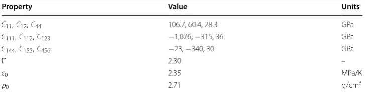
Thermoelastic properties for aluminum are listed in Table 1 [6]. For crystals of cubic symmetry, ŴIJ =ŴδIJ, in indicial notation.

The plastic velocity gradient is, summing over slip systems k with initial slip direction sk and plane normal mk,

Here, the magnitude of the Burgers vector is b, the mobile dislocation density is N_mk with glide velocity v¯k, and the rate of homogeneous nucleation is N˙_homk with a mean glide dis-placement x¯. For FCC Al, slip occurs on up to k=1, 2,. . ., 12{111}�110� systems, and

(4)

EE ₌ 1

2

FETFE₋1_.

(5)

U

EE_,η

= 12CαβE E αEEβ+

1 6CαβδE

E

αEEβEEδ −θ0

ŴαEαE�η−f(�η)

.

(6)

f =exp(�η/c0)−1≈�η+12(�η) 2_/c0,

(7) σ

σσ ₌JE−1FE_(∂U/∂EE)FET_, θ ₌∂U/∂η.

(8) LP _{= ˙}FPFP−1₌

k

bN_mkv¯k_{+ ˙}N_homk x¯sk_⊗mk.

Table 1 Thermoelastic properties of Al (θ0₌300K)

Property Value Units

C11,C12,C44 106.7, 60.4, 28.3 GPa

C111,C112,C123 −1,076, −315, 36 GPa

C144,C155,C456 −23, −340, 30 GPa

Ŵ 2.30 –

c0 2.35 MPa/K

the corresponding ambient shear modulus is µ0=C44+ 1₃(C11−C12−2C44), leading to an initial shear wave velocity of cs=√µ0/ρ0; in the model, cs and µ are also updated with temperature and elastic strain [10]. The total dislocation density is Nk ₌N_mk ₊N_ik, where N_ik is the immobile density. Constitutive relations for the crystal-level mobile and immobile dislocation density evolution, as well as their associated mean veloc-ity, build upon on previously developed isotropic constitutive models [3, 8, 9]. Letting τk =σσσ :(FEsk_⊗mkFE−1_{) denote the resolved Cauchy stress on system k, evolution} equations are [6]

Density rates corresponding to homogeneous nucleation, heterogeneous nucleation, multiplication, annihilation, and trapping are labeled by obvious subscripts. Densities of forest and parallel dislocations are, respectively,

Dislocation velocities are controlled by the following relations [6, 10] that involve phys-ics of thermal activation at low stress and viscous drag at high stress:

(9)

˙

N_mk =χN˙_homk + ˙N_hetk + ˙N_mulk − ˙N_annk − ˙N_trak ,

(10)

˙

N_ik =(1−χ )N˙_homk + ˙N_trak

(11)

˙

N_homk = ˙N0expg0homµb3/kBθ

|τk_|/τ_0hom−1,

(12)

˙

N_hetk =α_{het| ˙}τk_|(m+1)

|τk_{| −}τmin

m

/(τmax−τmin)1+m

ifτ_{min≤ |}τk_{| ≤}τ_max N˙_hetk =0 otherwise,

(13) ˙

N_mulk =pmulNmk

N_fk|¯vk|,

(14) ˙

N_annk =2αannb

N_mk2|¯vk|,

(15) ˙

N_trak =α_traN_mk

N_fk|¯vk|.

(16)

N_fk = l

Nl m

k

·ml_×sl , N

k p =

l Nl

m

k

×ml_×sl .

(17) ¯

vk = csh k

[exp(�Gk_/k

Bθ )−1][cshk(N_fk)1/2/νG] +1

if|τk|> τpas (v¯k =0 otherwise),

(18)

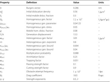
Parameters entering (9)–(20) are compiled in Table 2; for a more thorough description of the dislocation density based framework for slip, see [6, 10, 22].

The present FD scheme permits particle displacements in all three Cartesian direc-tions, but variations in displacement are permitted only in the direction of wave propa-gation denoted X1, leading to the following matrix form of deformation gradient (1):

Balances of momentum and energy are often augmented with a scalar artificial viscosity q; correspondingly, from (2) and (3), for deformation of the form (21),

Letting subscripts followed by commas denote spatial discretization indices and super-scripts denote temporal discretization indices, t and X1 the fixed time step and grid spacing, in discretized form (22)–(24) are

(19)

τ_pask ₌αpasµb

Nk

p, τcutk =αcutµ0b

N_fk,

(20) hk = [(ξk)2+1]1/2−ξk, ξk =B0cs/(2τkb).

(21)

[F] = 



∂x1/∂X1 0 0 ∂x2/∂X1 1 0 ∂x3/∂X1 0 1



= 



F11 0 0

F21 1 0

F31 0 1 



(22) ∂Fi1/∂t=∂υi/∂X1,

(23)

ρ0(∂υi/∂t)=∂Pi1/∂X1−(∂q/∂X1)δi1,

(24) ∂U/∂t=(Pi1−qδi1)Fi˙1.

Table 2 Plastic properties of Al (θ0₌300K)

Property Definition Value Units

b Burgers vector 0.286 nm

N₀k Initial dislocation density 0.56 1/µm2

f0 Initial mobile disloc. fraction 0.3 –

˙

N0 Homogeneous gen. factor 7.2×107 1/(µm2µs)

g0hom Homogeneous gen. parameter 0.04125 –

τ0hom/µ0 Homogeneous gen. stress 0.05 –

χ Mobile hom. disloc. fraction 0.08 –

¯

x/b Generation displacement 13.3 –

αhet Heterogeneous gen. factor 320 1/µm2

m Heterogeneous gen. exponent 0.8 –

τmin/µ0 Heterogeneous gen. bound 0.004 –

τmax/µ0 Heterogeneous gen. bound 0.04 –

pmul Multiplication probability 0.088 –

αann Annihilation factor 0.25 –

αtra Trapping factor 0.051 –

αpas Passing strength factor 0.1 –

αcut Cutting strength factor 0.9 –

νG Obstacle attempt frequency 1×105 1/µs

B0 Drag coefficient 18.0 Pa µs

Artificial viscosity (linear + quadratic) is computed as

with �υ_1,n+_i+1₁/2_/2=υ_1,n+_i+1₁/2−υ_1,n+_i1/2, c_l the longitudinal linear elastic wave speed, a1=0.06, and a2=2.0. During expansion/rarefaction (ρ_in₊+₁1_/2−ρ_in_+1/2<0 ) , q=0; note q≥0 follows from (28). The linear viscosity coefficient a1 was chosen small enough to not influence the shock structure, whereas quadratic coefficient a2 was chosen so that the shock would spread over three to five elements [28].

Steady wave model

The theory implemented in the current SW simulations [10, 11] is essentially equivalent to that of “Finite difference model”, Eqs. (1)–(20) and properties in Tables 1 and 2. As dis-cussed in detail in Ref. [10], the SW model invokes the Helmholtz free energy as the fun-damental thermodynamic potential, related to internal energy U via the partial Legendre transformation

Stress and entropy obey

Correspondences among properties in Table 1 and those entering a free energy function consistent with (5) (e.g., cubic in strain) are achieved via the usual Maxwell relations of nonlinear Lagrangian thermoelasticity [23, 29].

In contrast to (21), for the SW model it is assumed deformation is uniaxial and of the form below with F11=:

and is unable to model transverse waves captured by the FD method of “Finite difference model”. However, also in contrast to the FD approach, no artificial viscosity is required for strong shocks, and the shock profile (e.g., width) is an outcome of the simulation (25)

F_i1,in+₊1_1/2−F_i1,in _+1/2/�t₌υ_i,in+₊1/2_{1 −}υ_i,in+1/2 /�X1, (26) ρ0 �t

υ_in+1/2₋υ_in−1/2₌ 1 �X1

P_in_1,i+1/2−q_in₊−₁1_//₂2δ_i1

−Pn_i1,i−1/2−q_in₋−₁1_//₂2δ_i1

,

(27) U_in₊+₁1_/2−U_in₊1/2=

1 2

P_i1,in+1_+1/2+P_i1,in ₊1/2

−q_in₊+₁1_//₂2δi1

F_i1n+1−F_i1n

.

(28) qn_i++₁1_//₂2= 12

ρ_in₊+₁1_/2+ρ_in_+1/2

a1cl|�υn+ 1/2

1,i+1/2| +a2|�υ n+1/2 1,i+1/2|

2

,

(29)

�₌�

EE_,θ

=U−θ η.

(30) σ

σσ ₌JE−1FE

∂�/∂EE

FET_, η_{= −}∂�/∂θ.

(31)

[F_{] =}





∂x1/∂X1 0 0

0 1 0

0 0 1



= 

 _{0 0}

0 1 0 0 0 1



rather than controlled by viscous regularization. Equations of continuity and momen-tum conservation reduce to

Introducing a coordinate Y =X1−Dt moving with steady speed D in the (X1-) direc-tion of shock propagadirec-tion, partial differential equadirec-tions in (32) can be transformed to the ordinary differential equations

Similarly, rate equations for plastic deformation, dissipative temperature rise, and dislo-cation densities become

Here, θ ₌θ0+�θE+�θP, where �θP results from plastic work and �θE results from thermoelastic coupling (see [10] for full expressions). Integration of (33) from +∞ gives the Raleigh line

where (_·)+ denotes a quantity evaluated at the beginning of the steady plastic wave; for a weak shock, this state corresponds to the elastic precursor and HEL; for a strong/ overdriven shock, P₁₁+ =0 and +_{=1. In the numerical implementation, (34)–(36) are}

solved incrementally along the Raleigh line from the initial state (_·)+ to the end state (_·)− , where the latter is determined by the imposed boundary condition (e.g., shock stress P₁₁− or volume ratio V−/V0=− in the final shocked state at Y → −∞). The material response may be fully anisotropic, but the analysis ignores transverse waves that would arise from loading along crystal orientations with less than two-fold rotational symme-try [30] (neglecting nonlinear elastic effects from higher order elastic constants that may introduce longitudinal and transverse wave coupling [31]).

Analytical model

The present method of analytical solution, described more fully in Ref. [15], considers the Rankine–Hugoniot jump conditions for a steady planar shock [12]:

These conditions, which idealize the shock structure to infinitesimal thickness, effectively replace (3). The above conditions consider a continuous and initially homogeneous slab of material through which a planar shock moves, in the X1-direction, with natural veloc-ity D. As in “Steady wave model”, let (_·)+ and (_·)− label quantities in the material ahead (i.e., upstream) and behind (i.e., downstream) from the shock. Let [[(_·)_{]] =}(_·)−₋(_·)+ and �(_·)_{� =} 1_2[(_·)−₊(_·)+_] denote the jump and average of a quantity across the shock. Let n be a unit normal vector to the planar shock, i.e., n₌∂x/∂x1. The only nonvanishing

(32) ∂υ1/∂X1=∂/∂t, ∂P11/∂X1=ρ0(∂υ1/∂t).

(33)

dυ1/dY = −Dd/dY, dP11/dY = −ρ0D(dυ1/dY).

(34)

dFP/dY = −LPFP/D, d(�θP)/dY = − ˙θP/D,

(35) dN_mk/dY = − ˙N_mk/D, dN_ik/dY = − ˙N_ik/D.

(36)

P11−P₁₁+ =ρ0D2(₋+),

(37) [[ρv]] =0, [[σ]] −ρv[[v]] =0,

(38) [[ρv(u+ 12v

2₎

component of particle velocity is υ₌υυυ_·n. The Cauchy stress component normal to the shock front is σ ₌σσσ_:(n_⊗n)₌σ11. The relative velocity of the material with respect to the shock is v=υ−D. Internal energy per unit mass is u=U/ρ0. Using (37), (38) can be rewritten as [12]

The downstream state is defined by the set of variables (υ−,ρ−,σ−,u−). The Rankine– Hugoniot conditions give three equations for determining this state; in order to fully define the downstream state, a fourth equation is supplied by the constitutive model. Here, the constitutive theory for thermoelastic response is identical to the anisotropic nonlinear Lagrangian theory of “Finite difference model”, Eqs. (1), (4)–(7), and Table 1. Considered are longitudinal elastic–plastic shocks corresponding to planar impact in pure mode direc-tions in single crystals (i.e., direcdirec-tions parallel to an axis of two-fold or greater rotational symmetry). A sample of material subjected to a step or ramp loading in normal stress, with no applied shear stress, develops a two-wave structure consisting of a single longitudi-nal elastic wave (i.e., the elastic precursor), followed by a single longitudilongitudi-nal plastic wave of velocity D if the HEL is exceeded. For overdriven shocks, there is no precursor. Total deformation is

For the highly symmetric [100] orientation considered in “Comparison of numerical and analytical solutions”, n₌8 glide systems are active simultaneously at shock stresses exceeding the HEL stress PH = −σ+_{= −}P₁₁+, all at the same rate [13]. For monotonic loading, integration of (8) yields the plastic deformation:

with cumulative shear γ, which accounts for slip and nucleation contributions, to be determined as an outcome of the analysis. The exponential solution in the first of (42) is exact when the plastic shearing rate is constant, i.e., when γ˙ ₌γ /t=constant. The series

approximation in the second of (42) is accurate to third order in shear and was sufficient for problems considered here, where the maximum values of γ are on the order of 0.1. From the geometry of the problem, all n systems experience the same resolved shear stress τ ₌τk. In lieu of the viscoplastic model implemented in “Finite difference model” and “Steady wave model”, for the analytical treatment a two-parameter yield criterion in the plastically deforming regime is prescribed:

(39) [[u]] = �σ_�[[1/ρ_{]] ⇔ [[}U]] = �σ_�[[J]].

(40)

[F+_{] =}



 + _{0 0}

0 1 0 0 0 1



= [FE+],

(41)

[F−_{] =}



 − _{0 0}

0 1 0 0 0 1 

= [FE−FP−].

(42)

FP(γ )₌exp

γ

k

sk_⊗mk

≈1_+γ k

sk_⊗mk₊ γ

2

2

k

sk_⊗mk 2

+γ

3

6

k

sk_⊗mk 3

Here, g0 is dimensionless initial shear strength at the HEL, dependence of strength g =gk on temperature is omitted, and hardening is proportional via constant H to the total slip on all n active systems. The factor of J =JE in (43) accounts for work conjugacy of Kirch-hoff stress and plastic slip in the intermediate configuration implied by the multiplicative decomposition of F in (1) [23].

Assume that HEL shock stress PH is known from experiment. Then the upstream

(HEL) state is fully determined by the analytical solution in Refs. [16, 29]. Specifically, is decreased incrementally until _{P= −P11= −σ11} reaches _PH (positive in compres-sion), at which point ₌+ and _{U =U}+. Given total deformation − and slip variable γ, thermoelastic deformation behind the plastic shock is known from FE ₌F(−)FP−1(γ ) . Internal energy, axial shock stress, and shear stress can then be written as

Note that the full thermoelastic constitutive model is required for evaluation of (44). Let −_=V−_/V0 be prescribed as the load parameter. Then energy balance (39) and yield criterion (43) comprise two coupled algebraic equations that can be solved simultane-ously for γ and η−:

To obtain Hugoniot stress versus volume curves, (46) and (45) are solved simultaneously for γ and η− as − is decreased incrementally from the HEL state. With shock stress com-puted from the second of (44), plastic shock velocity D and downstream particle velocity υ− can be obtained from the Hugoniot equations for mass and momentum conservation in (37), leading to [7]

The downstream state is now fully known. For aluminum single crystals, the first strength parameter g0=7.2×10−4 is known from the nonlinear elastic solution [16] at PH =0.1 GPa [10], corresponding to +_≈0.999, and thus does not require calibration. The second parameter, hardening constant H =0.05, is calibrated such that cumulative plastic deformation predicted by the analysis for shocks in the regime PH ≤P−≤25 GPa is in respectable agreement with that predicted by the numerical methods of “Finite difference model” and “Steady wave model”, which have been compared extensively to experiments [6, 10]. The calibration of H will be explained later in “Comparison of numerical and analytical solutions”. Much of the foregoing discussion applies for weak shocks; for strong shocks, conditions PH →P+=0, +=1, υ+=0, and U+=0 are enforced.

Numerical methods comparison

Approximations introduced by the FD and SW numerical methods are evaluated quan-titatively via examination of results of four representative test problems, whose shock

(43) Jτ/µ0=g(γ )/µ0=g0+Hnγ.

(44) U−=U−(−_,γ,η−), P−=P−(−_,γ,η−), τ ₌τ (−_,γ,η−).

(45) U−(−_,γ,η−)₋U+= 12[P−(F−,γ,η−)+PH][+−−],

(46) τ (−_,γ,η−_{)/µ0=(g0+Hnγ )/}−_.

(47)

strengths are given in Table 3. Because the SW method approximates strain as uniaxial, it is expected to give highly accurate solutions for impact problems wherein the target is shocked along a direction that possesses twofold or greater rotational symmetry (which results in uniaxial strain), and give approximate solutions for problems of lower symmetry (in which quasi-longitudinal and quasi-transverse may form). The FD method is able to model weak shock loading problems without an artificial viscosity given a mesh resolution that can sufficiently resolve the shock width; however, in the strong shock regime viscous regularization is used to damp the large jump in velocity that precedes plastic deforma-tion [6]. The approximations associated with each of the four problems are summarized in Table 3. In low symmetry simulations, the crystal is rotated from the reference frame via Bunge angles φ1=43.7◦, =49.26◦, and φ2=132.8◦, producing the orientation in Fig-ure 1. The FD mesh resolution (�X1) is fixed, and a consistent step size is chosen for SW simulations so that approximately the same number of points is used to resolve the SW in all simulations.

Velocity profiles

In FD simulations at P−_{=5 GPa, the shock was generated by longitudinal plate impact} of an a-sapphire impactor (X-cut). In all FD simulations, the a-sapphire impactor was modeled using isentropic thermoelasticity with an internal energy potential third order in elastic Green strain and elastic constants from Ref. [32]. The shock response was sam-pled from an interior point located 5.0 mm from the impact surface for these simulations, which were discretized using a mesh resolution of X1=0.83µm. Velocity profiles from the SW and FD simulations of [100] and low symmetry orientations are compared in Fig-ure 2. Because SW simulations are based on relative time, the wave profile is adjusted so that it is centered on the FD solution, which uses total time after impact.

For the [100] orientation, Figure 2a indicates that the SW and FD simulations give nearly identical results. This agreement is expected as neither method introduces Table 3 Numerical simulations and approximations

Simulation SW approximations FD approximations

5 GPa [100] None None

5 GPa low symmetry Uniaxial F None

25 GPa [100] None Artificial viscosity

25 GPa low symmetry Uniaxial F Artificial viscosity

intrinsic approximations for this orientation and shock strength (Table 3). For the low symmetry orientation, Figure 2b shows that although the SW method approximates deformation as uniaxial, it predicts a nearly identical longitudinal component of the velocity profile as the FD simulation. Although the wave profiles are nearly identical, the SW method under-predicts the peak resolved shear stress that occurs on slip systems by approximately 10% because it does not include the shear components of the quasi-longi-tudinal wave [22]. However, this appears to negligibly influence the longitudinal compo-nent of the velocity profile at the low impact stress.

In FD simulations at P−=25 GPa, the shock was again generated by longitudinal plate impact via an a-sapphire impactor; however, in this case an artificial viscosity was used. The shock response was sampled from an interior point located 20.0µm from the impact surface for these simulations, which were discretized using a mesh resolution of X1=5.0 nm. Velocity profiles from the SW and FD simulations of [100] and low sym-metry orientations are compared in Figure 3.

For the [100] orientation, wave profiles for the two methods are shown in Figure 3a. Because the SW method begins to track the solution at an adiabatic elastic compression for which the longitudinal elastic wave speed equals the SW speed (in this case, at a par-ticle velocity of approximately 0.55 km/s), it gives no additional information concerning

the wave profile up to this velocity; however, any wave structure calculated by the FD method up to this velocity is due to the artificial viscosity, so no physical insight is gained in FD simulations up to this velocity either. Above this velocity, the SW method predicts a slightly sharper rise than the FD method. This is because even though an extremely fine mesh resolution is employed there is still a smearing effect from the artificial viscos-ity, which decreases the peak strain rate experienced in the material. This decrease in peak strain rate decreases the rate of homogeneous dislocation by two orders of mag-nitude, which in turn alters the wave profile at elevated velocities, as fewer mobile dis-locations are available to relax the deviatoric response through glide. Even though the coupling between viscoplasticity and viscous regularization is undesirable, the FD and SW methods predict nearly identical strength and accumulated plastic strain, although their wave profiles differ slightly.

Computed wave profiles for the low symmetry orientation in Figure 3b differ in several respects. The FD method captures transverse components of formation of the quasi-lon-gitudinal wave which cannot be considered using the SW method. Additionally, the FD method predicts a single wave structure, whereas the SW method indicates deformation preceding the main rise. As discussed previously, local adiabatic treatment of overdriven shocks provides no information until the point where the elastic wave speed equals the

SW speed. However, for the low symmetry shock, since SW simulation (longitudinal wave) has a different elastic stiffness than the FD simulation (quasi-longitudinal wave), the point where viscoplastic deformation occurs differs. This causes the two methods to predict differing shock structures, where the SW method predicts a dual shock structure and the FD method predicts an overdriven shock. Additionally, the FD method expe-riences elevated shear stresses due to the transverse deformation components, which gives a slightly different viscoplastic response as well. Based on these observations, the SW method appears unsuitable for simulations in which transverse wave components have a relatively large magnitude, i.e., simulation of strong shocks in single crystals with low symmetry orientations.

Computational efficiency

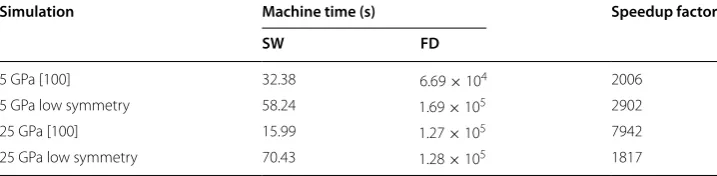
Because the SW method converts governing partial differential equations in space-time to ordinary differential equations in a steadily moving coordinate frame, it is expected to be significantly more computationally efficient than the FD method. This assertion is verified by computation times for simulations described in “Velocity profiles”. Table 4 shows that the SW method is ≈2,000–8,000× faster than the FD method.

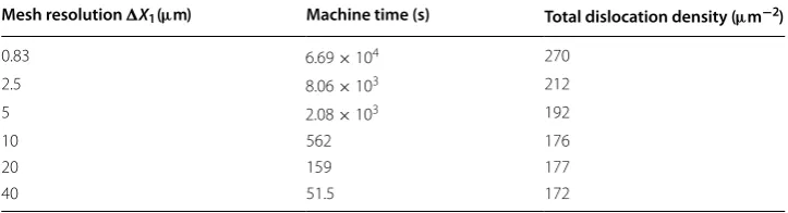
For the FD simulations presented in this work, one reason that the total computation times are several orders of magnitude longer than SW simulations is that a sufficiently fine mesh is employed so that dissipation is primarily due to the viscoplastic constitu-tive equation and not from artificial viscous regularization. To illustrate the effect of mesh resolution and viscous regularization on the wave profile, FD simulations were performed on a [100] single crystal shocked at P−_{=5 GPa. The resultant wave profiles} are given in Figure 4 whereas computation times and computed dislocation densities in the shocked state are given in Table 5. Figure 4 illustrates that when an artificial vis-cosity is employed in conjunction with a mesh resolution that is too coarse to resolve the shock width predicted from the viscoplastic constitutive relations alone, the shock is smoothed. Consequently, Table 5 indicates that although computation times approach those associated with the SW method, the viscoplastic behavior, indicated by the total dislocation density in the shocked state, is altered due to the decrease in peak strain rate associated with the shock. When this damping occurs the viscoplastic behavior becomes highly mesh-dependent. Consequently, physical meaning associated with internal state variables that govern viscoplastic deformation and the ability to predict detailed wave profile evolution are lost in the FD approach with nonzero artificial viscosity.

Although the analysis in this section used a fixed set of shock viscosity parame-ters (recall a1=0.05 and a2=2.0), without significantly decreasing these parameters

Table 4 Total computation times on a single 2.67 GHz Intel Xeon X5650 processor

Simulation Machine time (s) Speedup factor

SW FD

5 GPa [100] 32.38 6.69_×104 ₂₀₀₆

5 GPa low symmetry 58.24 1.69_×105 2902

25 GPa [100] 15.99 1.27_×105 ₇₉₄₂

a similar conclusion is reached. In cases where mesh resolution is not fine enough to resolve the viscoplastic shock behavior, the shock is smoothed across three to five ele-ments by the quadratic component of the viscosity. The quadratic viscous pressure is proportional to the square of the jump in velocity, so unless a2 is altered by orders of magnitude, the viscous pressure is determined by the magnitude of the velocity jump, and not by the relative magnitude of a2.

Comparison of numerical and analytical solutions

Aspects of numerical solutions obtained using the FD approach of “Finite difference model” and the SW approach of “Steady wave model” are now compared with available results from the analytical approach outlined in “Analytical model”. Specifically, the analy-sis is applied towards pure Al single crystals shocked along [100] to stresses of P−=5 GPa and P−_{=25 GPa, the former corresponding to a weak plastic shock with an elastic} pre-cursor and the latter to a single overdriven plastic wave. Tables 6 and 7 list outcomes of the computation/analysis—volume ratio, resolved shear stress, cumulative plastic strain, total temperature rise, particle velocity, and shock velocity—for shocks of strength 5 and 25 GPa, respectively, obtained from the FD method, SW method, and analytical solution.

Figure 4 Longitudinal velocity υ1 computed using FD method with varying mesh resolution compared with SW method predictions (P−=5 GPa). All FD simulations used an artificial viscosity, (28), except

X1=0.83µm.

Table 5 Computational time and  total dislocation density for  [100] shock at P−₌5 GPa computed using the FD method with varying mesh resolutions

Mesh resolution _X1 (µ_m) Machine time (s) _{Total dislocation density (µm}−2₎

0.83 6.69_×104 ₂₇₀

2.5 8.06_×103 212

5 2.08_×103 ₁₉₂

10 562 176

20 159 177

The precursor velocity calculated from the analytical nonlinear elastic solution [16, 29] is 6.28 km/s, which is exceeded by D for the overdriven shock at P−=25 GPa. Also shown

for comparison are hydrodynamic predictions obtained using the Birch–Murnaghan pres-sure–volume equation of state (EOS) [33], with compressibility properties of Al from the literature [34]. Temperature rise in the EOS was calculated assuming compression is isentropic and internal energy is first order in entropy. The hydrodynamic approximation, which by construction omits shear/deviatoric stress components, is often used as a simple model for shocks in materials whose strength is low relative to shock pressure.

The analytical solutions are obtained nearly instantaneously, in contrast to the more computationally intensive numerical methods. However, the analytical solutions only apply for symmetric orientations for which a single slip variable γ suffices (e.g., [100] for FCC crystals). While the yield condition used in the analytical solution benefits from extreme simplicity, explicit rate and temperature effects on flow stress are ignored. Fur-thermore, while only a single fitting parameter (H) is required, rather than an extensive list as in Table 2, H must still be prescribed via comparison with shear strength data from experiments or other more physically descriptive model output. Here, following the latter approach, H has been calibrated such that cumulative plastic deformation

predicted by the analysis for 5 and 25 GPa shocks is in relatively close agreement (within ≈20% error) with that predicted by SW and FD models, as is evident from Tables 6 and 7. Results for all end state variables and shock velocity are nearly equal for FD and

(48) ¯

ǫ_effP ₌

� 2 3

� _�

LP_sym:LP_sym �1/2

dt=

� 2 3

� _�

DP _:DP �1/2 dt =γ � � � � � 2 3 � ₈ � i=1

(si_⊗mi₎ sym � :   8 � j=1

(sj_⊗mj₎ sym





Table 6 Shocked state of Al [100] (P−

=5 GPa)

Variable (units) FD SW Analytical Birch–Murnaghan EOS

− _{0.944 0.944 0.945 0.944}

τ− (MPa) 56.7 55.8 120.4 0

(ǫ¯effP )− 0.037 0.037 0.034 0

(�θ )− (K) 40.5 39.2 42.3 38.36

υ− (km/s) 0.323 0.323 0.319 0.321

D (km/s) 5.739 5.717 5.798 5.771

Table 7 Shocked state of Al [100] (P−

=25 GPa)

Variable (units) FD SW Analytical Birch–Murnaghan EOS

− 0.810 0.805 0.805 0.816

τ− (GPa) 1.023 1.047 0.417 0

(ǫ¯effP )− 0.113 0.110 0.131 0

(�θ )− (K) 256.1 269.1 250.8 126.56

υ− _{(km/s) 1.324 1.341 1.343 1.303}

SW simulations. Because these or very similar values have already been compared with experimental data [18, 19, 35–39] indicative of viscoplastic relaxation rates (e.g., strength, precursor decay, wave profiles in single crystals and polycrystals) in previous publications [6, 10], these numerical results are deemed physically accurate. Results for volumetric compression ratio, adiabatic temperature rise, particle velocity, and shock velocity obtained from the analytical solution are also very close to correspond-ing numerical results, and effective plastic strain is reasonably close as noted already, although it is reiterated that the hardening parameter H entering the analytical method is obtained by fitting plastic deformation to the FD results. The only major discrepancy between analytical and numerical solutions is slip system-level shear strength in the shocked state (τ−), which appears to be over-predicted by the analytical solution for the 5 GPa shock and under-predicted for the 25 GPa shock. While it would be possible to more closely duplicate results of the numerical methods by using a more complex (i.e., nonlinear) hardening model than that prescribed in (43), such an approach would also suffer from requiring additional fitting of more parameter(s), detracting from the sim-plicity of the analytical approach. Similarly, using a simple viscoplastic model wherein the dislocation density and velocity are prescribed functions of the accumulated shear strain and shear stress, respectively, may produce results that are simpler to replicate using the analytical model [5]. However, such a model is unable to describe both the weak and strong shock loading regimes [9]. Previous isotropic representations [3, 7–9] are also unable to account for anisotropy of single crystals and textured polycrystals that are addressed by the present fully anisotropic theory.

Because the Birch–Murnaghan EOS assumes a spherical stress state, shear stress and plastic deformation are unresolved in Tables 6 and 7, and temperature rise is under-pre-dicted since there is no contribution to dissipation from plastic slip. The EOS does, how-ever, predict reasonably accurate values of relative volume, particle velocity, and shock velocity.

Conclusion

Analytical, FD, and SW numerical solutions have been compared for shock loading of single crystals using identical thermoelastic frameworks, but with rate- and temperature-independent shear strength constitutive relations in the analytical approach, and rate- and temperature-dependent shear strength constitutive relations in the latter two methods. Scenarios exist in which each of these methods is most appropriate. These method com-parisons have not been published in previous papers which have focused on each model and its results in isolation.

On the other hand if there is data that quantifies the spatio-temporal of the velocity profile, or if rate-dependent micromechanical mechanisms that govern the viscoplastic material response are well characterized, the SW or FD methods may be more appropri-ate. In particular, the SW and FD methods can be used to predict the steady shock struc-ture as well as give information regarding evolution of internal state variables and the thermodynamic state prior to, within, and after the shock. Due to its computational effi-ciency, the SW method is especially useful for developing constitutive equations prior to their implementation in FD frameworks. Additionally, in “Computational efficiency” it was shown that predicted rate-dependent behavior may be unphysically altered in FD simulations due to viscous damping effects unless a sufficiently fine mesh resolution is employed, whereas viscous damping is not required in the SW method. Only the FD method is capable of quantifying transient aspects of evolving shock waves, which is necessary to model spatio-temporal shock wave evolution data such as elastic precursor decay.

All three methods can be used to model highly symmetric single crystal orientations subjected to shock loading, but only the FD method can be used to capture quasi-longi-tudinal and quasi-transverse waves that arise in low symmetry crystal orientations. For weak shock loading in Al, approximating deformation as uniaxial was shown to be rea-sonable. Therefore, the SW method should be preferred due to its computational effi-ciency and lack of artificial viscosity. For strong shocks, however, the response of low symmetry crystal orientations was poorly captured using the SW method. Therefore, when modeling strong shocks for low symmetry crystal orientations relative to the load-ing direction, the finite-difference method should be employed.

These conclusions can be extended to other cubic metals with similar elastic anisot-ropy. However, additional investigations are required before generalizing these conclu-sions to materials that exhibit significantly higher elastic anisotropy or materials with lower crystal symmetry.

Authors’ contributions

JTL performed finite difference and steady wave simulations. JDC derived and calculated the analytical shock response. RAA and DLM helped create, derive, and evaluate the viscoplastic formulation in conjunction with JTL. All authors read and approved the final manuscript.

Author details

1 _{Impact Physics Branch, US Army Research Laboratory, Aberdeen Proving Ground, MD 21005-5066, USA.} 2 _Materials

Modeling and Simulation Group, Lawrence Livermore National Laboratory, Livermore, CA 94550, USA. 3 _{Woodruff School}

of Mechanical Engineering, Georgia Institute of Technology, Atlanta, GA 30332-0405, USA. 4 _{School of Materials Science}

and Engineering, Georgia Institute of Technology, Atlanta, GA 30332-0405, USA.

Acknowledgements

The authors would like to thank Dr. Richard Becker for stimulating discussions concerning implementation of the FD method. This work was performed, in part (RAA), under the auspicies of the US Department of Energy by Lawrence Livermore National Laboratory under contract DE-AC52-07NA27344 (LLNL-JRNL-663743). DLM is grateful for the support of the Carter N. Paden, Jr. Distinguished Chair in Metals Processing.

Compliance with ethical guidelines Competing interests

The authors declare that they have no competing interests.

References

1. McQueen RG, Marsh SP, Taylor JW, Fritz JN, Carter WJ (1970) The equation of state of solids from shock wave studies. In: Kinslow R (ed) High velocity impact phenomena. Academic Press, New York, pp 293–417

2. Herrmann W, Hicks DL, Young EG (1971) Attenuation of elastic–plastic stress waves. In: Burke J, Weiss V (eds) Shock waves and the mechanical properties of solids. Syracuse University Press, New York, pp 23–63

3. Clifton R (1971) On the analysis of elastic visco-plastic waves of finite uniaxial strain. In: Burke J, Weiss V (eds) Shock waves and the mechanical properties of solids. Syracuse University Press, New York, pp 73–116

4. Johnson JN (1972) Calculation of plane-wave propagation in anisotropic elastic–plastic solids. J Appl Phys 43:2074–2082

5. Winey JM, Gupta YM (2006) Nonlinear anisotropic description for the thermomechanical response of shocked single crystals: inelastic deformation. J Appl Phys 99:023510

6. Lloyd JT, Clayton JD, Becker R, McDowell DL (2014) Simulation of shock wave propagation in single crystal and polycrystalline aluminum. Int J Plast 60:118–144

7. Molinari A, Ravichandran G (2004) Fundamental structure of steady plastic shock waves in metals. J Appl Phys 95:1718–1732

8. Austin RA, McDowell DL (2011) A dislocation-based constitutive model for viscoplastic deformation of fcc metals at very high strain rates. Int J Plast 27:1–24

9. Austin RA, McDowell DL (2012) Parameterization of a rate-dependent model of shock-induced plasticity for copper, nickel, and aluminum. Int J Plast 32–33:134–154

10. Lloyd JT, Clayton JD, Austin RA, McDowell DL (2014) Plane wave simulation of elastic–viscoplastic single crystals. J Mech Phys Solids 69:14–32

11. Lloyd JT, Clayton JD, Austin RA, McDowell DL (2014) Modeling single-crystal microstructure evolution due to shock loading. J Phys Conf Ser 500:112040

12. Germain P, Lee EH (1973) On shock waves in elastic–plastic solids. J Mech Phys Solids 21:359–382

13. Johnson JN (1974) Wave velocities in shock-compressed cubic and hexagonal single crystals above the elastic limit. J Phys Chem Solids 35:609–616

14. Perrin G, Delannoy-Coutris M (1983) Analysis of plane elastic–plastic shock-waves from the fourth-order anharmonic theory. Mech Mater 2:139–153

15. Clayton JD (2014) Analysis of shock compression of strong single crystals with logarithmic thermoelastic–plastic theory. Int J Eng Sci 79:1–20

16. Clayton JD (2013) Nonlinear Eulerian thermoelasticity for anisotropic crystals. J Mech Phys Solids 61:1983–2014 17. Thomas JF (1968) Third-order elastic constants of aluminum. Phys Rev 175:955–962

18. Huang H, Asay JR (2006) Reshock response of shocked aluminum. J Appl Phys 100:043514

19. Turneare SJ, Gupta YM (2009) Real time synchrotron X-ray diffraction measurements to determine material strength of shocked single crystals following compression and release. J Appl Phys 106:033513

20. Clayton JD (2009) A continuum description of nonlinear elasticity, slip and twinning, with application to sapphire. Proc R Soc Lond A 465:307–334

21. McGlaun JM, Thompson SL, Elrick MG (1990) CTH: a three-dimensional shock wave physics code. Int J Impact Eng 10(1):351–360

22. Lloyd JT (2014) Microstructure-sensitive simulation of shock loading in metals. Ph.D. thesis, Georgia Institute of Technology, Atlanta, GA

23. Clayton JD (2011) Nonlinear mechanics of crystals. Springer, Dordrecht

24. Luscher DJ, Bronkhorst CA, Alleman CN, Addessio FL (2013) A model for finite-deformation nonlinear thermome-chanical response of single crystal copper under shock conditions. J Mech Phys Solids 61:1877–1894

25. Clayton JD (2005) Dynamic plasticity and fracture in high density polycrystals: constitutive modeling and numerical simulation. J Mech Phys Solids 53:261–301

26. Becker R (2004) Effects of crystal plasticity on materials loaded at high pressures and strain rates. Int J Plast 20:1983–2006

27. Farren WS, Taylor GI (1925) The heat developed during plastic extension of metals. Proc R Soc Lond A 107:422–451 28. Wilkins ML (1980) Use of artificial viscosity in multidimensional fluid dynamic calculations. J Comput Phys

36(3):281–303

29. Thurston RN (1974) Waves in solids. In: Truesdell C (ed) Handbuch der Physik VIA/4. Springer, Berlin, pp 109–308 30. Waterman PC (1959) Orientation dependence of elastic waves in single crystals. Phys Rev 113(5):1240–1253 31. Winey JM, Gupta YM (2004) Nonlinear anisotropic description for shocked single crystals: thermoelastic response

and pure mode wave propagation. J Appl Phys 96:1993–1999

32. Winey JM, Gupta YM, Hare DE (2001) R-axis sound speed and elastic properties of sapphire single crystals. J Appl Phys 90:3109–3111

33. Birch F (1947) Finite elastic strain of cubic crystals. Phys Rev 71(11):809–824

34. Vinet P, Rose JH, Ferrante J, Smith JR (1989) Universal features of the equation of state of solids. J Phys Condens Mat-ter 1(11):1941–1963

35. Huang H, Asay JR (2007) Reshock and release response of aluminum single crystal. J Appl Phys 101(6):063550 36. Smith RF, Eggert JH, Jankowski A, Celliers PM, Edwards MJ, Gupta YM et al (2007) Stiff response of aluminum under

ultrafast shockless compression to 110 gpa. Phys Rev Lett 98(6):065701

37. Gupta YM, Winey JM, Trivedi PB, LaLone BM, Smith RF, Eggert JH et al (2009) Large elastic wave amplitude and attenuation in shocked pure aluminum. J Appl Phys 105(3):036107

38. Turneaure SJ, Gupta YM (2011) Material strength determination in the shock compressed state using X-ray diffrac-tion measurements. J Appl Phys 109(12):123510