Improved Differential Evolution with Shrinking Space Technique for Constrained Optimization

O R I G I N A L A R T I C L E

Improved Differential Evolution with Shrinking Space Technique

for Constrained Optimization

Chunming FU1•_{Yadong XU}2•_{Chao JIANG}1• _{Xu HAN}1• _{Zhiliang HUANG}1

Received: 4 May 2016 / Revised: 10 February 2017 / Accepted: 2 April 2017 / Published online: 24 April 2017 ÓThe Author(s) 2017. This article is an open access publication

Abstract Most of the current evolutionary algorithms for constrained optimization algorithm are low computational efficiency. In order to improve efficiency, an improved differential evolution with shrinking space technique and adaptive trade-off model, named ATMDE, is proposed to solve constrained optimization problems. The proposed ATMDE algorithm employs an improved differential evolution as the search optimizer to generate new offspring individuals into evolutionary population. For the con-straints, the adaptive trade-off model as one of the most important constraint-handling techniques is employed to select better individuals to retain into the next population, which could effectively handle multiple constraints. Then the shrinking space technique is designed to shrink the search region according to feedback information in order to improve computational efficiency without losing accuracy. The improved DE algorithm introduces three different mutant strategies to generate different offspring into evo-lutionary population. Moreover, a new mutant strategy called ‘‘DE/rand/best/1’’ is constructed to generate new individuals according to the feasibility proportion of

current population. Finally, the effectiveness of the pro-posed method is verified by a suite of benchmark functions and practical engineering problems. This research presents a constrained evolutionary algorithm with high efficiency and accuracy for constrained optimization problems.

Keywords Constrained optimizationDifferential evolutionAdaptive trade-off modelShrinking space technique

1 Introduction

Constrained optimization problems (COPs) widely exist in various scientific and engineering fields [1–3], such as mechanical design, path planning, etc. Perhaps it is not easy or difficult to obtain global optimal solutions by the traditional optimization techniques for some COPs involving nonlinear inequality or equality constraints, multi-modal and non-differential objective functions. Evolutionary algorithms (EAs) cooperated with constraint-handling techniques which have obtained more and more attention because of their flexibility, effectiveness and adaptability provide an effective and powerful avenue to cope with these COPs [4–6]. A large number of effective constrained optimization evolutionary algorithms (COEAs) have been proposed [7–9]. Recently, some representative constraint-handling techniques with EAs to solve COEAs have been summarized by COELLO [10]. The most gen-eral existing constraint-handling techniques are mainly categorized into three groups. Firstly, the method based on the penalty function aimed to transform a COP into an unconstrained one by adding a penalty term to the original objective function [11,12]. Secondly, the approach based on the feasibility-based criterion preferred to select the Supported by National Science Foundation for Excellent Young

Scholars, China (Grant No. 51222502), Funds for Distinguished Young Scientists of Hunan Province, China (Grant No. 14JJ1016), and Major Program of National Natural Science Foundation of China (Grant No. 51490662).

& Yadong XU

[email protected]

1 _{State Key Laboratory of Advanced Design and}

Manufacturing for Vehicle Body, Hunan University, Changsha 410082, China

2 _{School of Mechanical Engineering, Nanjing University of}

feasible solutions rather than the infeasible solutions into the next evolutionary process [13,14]. Thirdly, the method based on the multi-objective optimization technique aimed to transform the COPs into the unconstrained multi-ob-jective optimization problems and utilized multi-obmulti-ob-jective optimization technique to deal with the converted problems [15,16].

The performance of COEAs mainly depends on the constraint-handling techniques and EAs as the search optimizer. Differential evolution (DE) originally proposed by STORN and PRICE [17] was one of the most simple and powerful population-based evolutionary algorithms for global optimization. During the past two decades, different DE optimizers with constraint-handling techniques have been successfully developed to deal with different kinds of COPs. The first attempt was the constraint adaption with DE (CADE) algorithm which introduced multi-member individuals to generate more than one offspring by DE operators [18]. A cultural DE-based algorithm with the feasibility rule was proposed by LANDA and COELLO [19], which utilized different knowledge sources to influ-ence the mutant operator in order to accelerate conver-gence. A multi-member diversity-based DE (MDDE) algorithm where each parent generated more than one offspring to enhance the diversity of population was pre-sented by MEZURA-MONTES, et al [20] to solve COPs. The dynamic stochastic selection technique was put for-ward by ZHANG, et al [21] under the framework of multi-member DE. TESSEMA and YEN [11] designed an adaptive penalty formulation where the feasible proportion of the current population was utilized to tune the penalty factor. In order to combine the advantages of different constraint-handling techniques, MALLIPEDDI, et al [22] proposed an ensemble of constraint-handling techniques (ECHT) with DE and evolutionary programming optimiz-ers for coping with COPs. ELSAYED, et al [23] introduced an algorithm framework to use multiple search operators in each generation with the feasibility rule for COPs. Each combination of search operators had its own sub-popula-tion, and the size of each sub-population varied adaptively during the progress of evolution depending on the repro-ductive success of the search operators. Subsequently, GONG, et al [24] developed a ranking-based mutation operator with an improved dynamic diversity mechanism for COPs. A modified differential evolution algorithm [25] was proposed to deal with the dimensional synthesis of the redundant parallel robot problem.

Recently, the adaptive trade-off model (ATM) [26] has been proposed to maintain a reasonable tradeoff to select better individuals to reserve into next generation between the feasible and infeasible individuals. The principal merit of ATM was that the promising infeasible individuals could be inherited into the next evolutionary process. The

ATM with evolutionary strategy (ATMES) as the search optimizer has been utilized to solve COPs. In order to reduce the computational effort, the shrinking space tech-nique introduced by AGUIRRE, et al [27] shrank the search region according to some feedback information and directed the search effort to the promising feasible region. Subsequently, WANG, et al [28] proposed a new method named AATM with high efficiency which benefited from the virtues of shrinking space technique and ATM. The performance of AATM algorithm could promptly converge to optimal results without loss of quality and precision.

Although AATM enhances the performance of ATMES by taking advantage of the shrinking space technique to address complicated COPs with multiple constraints, it still leaves a plenty of room to develop new approaches to solve COPs for improvement of accelerating the convergence rate and enhancing the quality of solutions within the limited time, especially for complicated engineering opti-mization problems. When using EAs to solve COPs, the search algorithm plays a crucial role on the performance of hybrid approaches as well as the constraint-handling techniques. Hence, this study employs an advanced search algorithm (i.e. an improved DE) to further improve the performance of AATM. The improved DE employs three different characteristic mutant strategies to generate dif-ferent offspring into evolutionary population. Hence, combining the advantages of an improved differential evolution with adaptive trade-off model and shrinking space technique, called ATMDE, is proposed to deal with COPs. The remainders of this paper are organized as fol-lows. In Section2, the definitions of COP and some rele-vant concepts of multi-objective optimization are given, respectively. In Section 3, the basics of DE are briefly introduced. In Section4, the proposed ATMDE algorithm is presented in detail. In Section5, the performances of ATMDE are tested by 18 well-known benchmark test functions from the 2006 IEEE Congress on Evolutionary Computation (IEEE CEC2006) and several engineering optimization problems. Section6concludes this paper.

2 Statement of the Problem

A general constrained optimization problem is formulated as

minfðxÞ;

s:t: gkðxÞ 0; k¼1;2; ;q;

hkðxÞ ¼0; k¼qþ1;qþ2; ;m;

_ð1Þ

wheref(x) is the objective function;g(x) andh(x) are the inequality and equality constraints, respectively;

variables and their allowable lower and upper boundaries arexmin,jandxmax,j(j=1, 2,,n);mis the total number of constraints;qandm-qare the numbers of inequality and equality constraints, respectively. In evolutionary opti-mization, equality constraints are transformed to inequality constraints as follows:

hkðxÞ

j j d0; ð2Þ

where d is a positive tolerance parameter and is recom-mended to be as 0.0001 [20,21].

In addition, the degree of violation value of solutionx

fromk-th constraintGk(x) is defined as

GkðxÞ ¼

maxf0;gkðxÞg; k¼1;2; ;q;

maxf0;jhkðxÞj dg; k¼qþ1;qþ2; ;m:

ð3Þ

Then, the degree of all the constraint violations of solutionxcan be represented as

GðxÞ ¼X

m

k¼1

GkðxÞ: ð4Þ

Since the following method utilizes the concepts of the multi-objective optimization techniques to address con-straints of COPs, some related multi-objective optimization concepts are introduced in advance.

Definition 1 Pareto dominance: A vectoru=(u1,u2,,

uk) is said toPareto dominateanother vectorv=(v1,v2,,

vk), denoted asuv, only if it is satisfied: 8i2 f1;2; ;kg; uivi and

9j2 f1;2; ;kg; uj\vj:

ð5Þ

Definition 2 Pareto optimality: u is said to be Pareto optimal only if vector v in the feasible region S doesn’t exist andvu, where v=f(v)=(f(v),G(v))=(v1,v2), u=f(u)=(f(u),G(u))=(u1,u2).

Definition 3 Pareto optimal set: The Pareto optimal set denoted asP*is defined as

P¼ fu2Sj:9v2S;vug: ð6Þ

It should be noted that individuals in the Pareto optimal set are callednon-dominatedindividuals.

Definition 4 Pareto front: The Pareto frontPF*is defined as

PF¼ ffðuÞju2Pg: ð7Þ

3 Basics of Differential Evolution

DE has been extensively applied to solve optimization problems because of its simplicity and effectiveness [17]. It does not require the binary encoding to represent solution

like genetic algorithm and not employ a probability density function to self-adapt its individuals like evolution strategy. It generates new candidate solutions by combining the parent individual and several other individuals of the cur-rent population. Then a candidate individual will replace the parent only if it has better fitness value. In the following text, the specific operations including initialization, muta-tion, crossover and selection are introduced. Firstly, it generates NP initial population xi (i=1, 2,, NP) sam-pled from the search domain by

xi;j¼xmin;jþrandð0;1Þ ðxmax;jxmin;jÞ; ð8Þ

where rand(0,1) means to generate a randomly real number between 0 and 1.

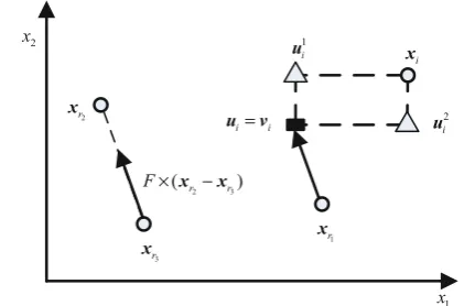
After initialization, a mutant strategy is adopted to generate a mutant vectorv_i=(vi,1,vi,2,,vi,n) by its cor-responding target vector xi=(xi,1,xi,2,,xi,n). There is a general nomenclature ‘‘DE/x/y’’ developed to denote the different DE mutant variants, where ‘‘DE’’ means differ-ential evolution, ‘‘x’’ indicates which individual as the base vector is selected to be mutated, and ‘‘y’’ is the number of difference vectors chosen for perturbation of x. The fol-lowing mutation strategies are most frequently used.

DE/rand/1:

vi¼xr1þF ðxr2xr3Þ: ð9Þ

DE/best/1:

vi¼xbestþF ðxr1xr2Þ: ð10Þ

DE/rand/2:

vi¼xr1þF ðxr2xr3Þ þF ðxr4xr5Þ: ð11Þ

DE/current-to-rand/1:

vi¼xiþF ðxr1xiÞ þF ðxr2xr3Þ: ð12Þ

DE/current-to-best/1:

vi¼xiþF ðxbestxiÞ þF ðxr1xr2Þ: ð13Þ

where indices r1,r2,r3, r4 andr5 are mutually exclusive

integers randomly selected from interval [1, NP] and are also different from individuali;Fis the scale factor chosen between 0 and 1; andxbestdenotes the best individual in the

current population.

Subsequently, a trial vector ui=(ui,1,ui,2,,ui,n) gen-erates by the binomial crossover or exponential crossover. The binomial crossover is utilized in this paper as follows:

ui;j¼

vi;j; if ðrandjð0;1Þ CRÞor j¼jrand;

xi;j; otherwise:

ð14Þ

where CR is the probability rate of crossover operator and jrandis a randomly integer chosen from the range [1,n]. The

strategy as an example, the schematic diagram of mutation and crossover operation is illustrated as shown Fig.1. The black square represents the mutant vector, which is the mutant vector u_i generated by mutant strategy. The two trianglesu1

i andu 2

i represent the two possible locations for

the trial vector after performing binomial crossover operation.

Then, the target vectorxi,gcompares with its trial vector

u_i,g by their fitness values, and the better one x_i,g?1will survive into the next generation population. The selection operation expresses as

xi;gþ1¼

ui;g; iffðui;gÞ fðxi;gÞ;

xi;g; otherwise:

ð15Þ

The above steps repeat generation by generation until the termination criterion is met.

4 Proposed Algorithm: ATMDE

The performance of COEAs mainly depends on the search ability of evolutionary algorithm and the effectiveness of constraint-handling technique. Hence, the proposed algo-rithm ATMDE utilizes an improved DE as search opti-mizer to reproduce offspring and introduces the adaptive trade-off model as the constraint-handling technique to select better individuals to retain into the next population. Furthermore, in order to reduce the redundant search region, the shrinking space technique is employed to enhance the convergence performance. This section will introduce the three core parts of ATMDE algorithm in detail, respectively.

4.1 Improved DE

To balance the convergence rate and accuracy of solution, an improved DE is used as the search engine for the pro-posed ATMDE algorithm. The set of offspring individuals

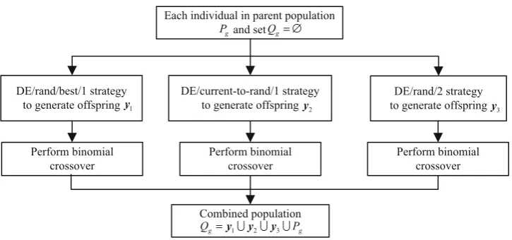
Qg is generated by the following three different mutant strategies (i.e. DE/rand/best/1, DE/current-to-rand/1, and DE/rand/2) which combine the advantages of different mutant strategies to generate individuals in order to increase the maximum probability of generating better offspring into evolutionary population. The strategies DE/ current-to-rand/1 and DE/rand/2 have the strong explo-rative ability to generate new promising individuals to add into the evolutionary population, and the strategy DE/rand/ best/1 has good exploitative ability to reproduce better individuals around the best individual. A good tradeoff between the global and local search performance can be achieved by combing the three different mutant strategies. The framework of generating offspring is shown in Fig.2. Each individual in the parent population is employed to generate three different offspring with three different mutant strategies and binomial crossover, and then the better individuals retaining into the next generation are chosen from the new offspring and parent population by ATM strategy.

The implementation of constructing ‘‘DE/rand/best/1’’ strategy is explained as follows. At the beginning, the ‘‘DE/ rand/1’’ strategy is introduced to maintain the diversity of population in order to prevent the population from being stuck in a local optimum. This strategy has the ability to enhance the global search ability because the new indi-viduals could learn the information from other indiindi-viduals randomly chosen from the whole population. Then it is necessary to accelerate the convergence of the evolutionary population, so the ‘‘DE/best/1’’ strategy is employed to speed up convergence as the feasibility proportion of cur-rent population increases. The ‘‘DE/best/1’’ strategy uti-lizes the information of the best individual in the current population to generate new individual which can enhance the convergence speed. Hence, the proposed strategy ‘‘DE/ rand/best/1’’ as shown in Algorithm 1 is constructed to balance diversity and convergence speed, which combines the ‘‘DE/rand/1’’ strategy and ‘‘DE/best/1’’ strategy through the feasibility proportion of current population. Specially, if a value randomly generated from [0, 1] is greater than the feasibility proportion of current population u, the ‘‘DE/rand/1’’ strategy is adopted. Otherwise, the ‘‘DE/best/1’’ strategy is employed.

Algorithm 1 The ‘‘DE/rand/best/1’’ strategy if rand(0, 1)[u, whereudenotes the feasibility proportion of current population

vi¼xr1þF ðxr2xr3Þ #DE/rand/1#

else

vi¼xbestþF ðxr1xr2Þ #DE/best/1#

end 1

x

2

x

3

r

x

2

r

x

2 3

( _{r r})

F× x −x

1

r

x

i

x

i= i

u v 2

i

u

1

i

u

4.2 Adaptive Trade-Off Model

Generally, a constraint-handling technique to address con-straints experiences three different situations in the whole evolutionary process: (1) the infeasible situation only includes the infeasible solutions; (2) the semi-feasible situ-ation includes the feasible and infeasible individuals simul-taneously; and (3) the infeasible situation only includes the infeasible individuals. The ATM strategy aims to construct an effective tradeoff scheme to address constraints for each situation according to their corresponding characteristics.

4.2.1 Infeasible Situation

In the infeasible situation, a hierarchical non-dominated selection strategy is introduced to choose individuals from Pareto front into the next population along with evolu-tionary process and is executed as follows: only the first half of non-dominated individuals with smaller constraint violations are selected to offspring population and are immediately eliminated from the parent population. This process repeats until the number of individuals reaches the size of the offspring population.

4.2.2 Semi-feasible Situation

In this situation, in order to balance the influence of objective value and constraint violation, the adaptive fitness transformation method is employed to calculate the fitness function ffit(xi) of individual xi. Firstly, the population is divided into the feasible individual group (Z1) and infeasible individuals group (Z2). The objective

function value f(xi) of solution xi is converted into

f0ðxiÞ ¼

fðxiÞ;i2Z1;

maxfufðxbestÞ þ ð1uÞfðxworstÞ;fðxiÞg;i2Z2;

ð16Þ

where f0ðxiÞis the converted objective function’s value of

solutionxi, andxbestandxworstare the best and worst solution

in the groupZ1, respectively. In order to assign equal

impor-tance to different objective functions, it is normalized as

fnorðxiÞ ¼

f0ðxiÞ min j2Z1[Z2

f0ðxjÞ

max

j2Z1[Z2

f0

ðxjÞ min j2Z1[Z2

f0

ðxjÞ

: ð17Þ

The constraint violation value calculated by Eq. (4) is also normalized as

GnorðxiÞ ¼

0; i2Z1;

GðxiÞ min j2Z2

GðxjÞ

max

j2Z2

GðxjÞ min j2Z2

GðxjÞ

; i2Z2:

8 > > < > > :

ð18Þ

Eventually, the final fitness function of solution xi is calculated by

ffitðxiÞ ¼fnorðxiÞ þGnorðxiÞ; i2Z1[Z2: ð19Þ

The individuals are ranked based on the values offfit()

in ascending order, and the individuals with smaller values are chosen to add into the offspring population until reaching its allowable size.

4.2.3 Feasible Situation

In this feasible situation, the constraint violations of COPs with zero are equivalent to be one of the unconstrained optimization problems because constraint violations of every individual are zero. Hence, only objective function is required to be considered, and Eq. (19) can be also used as a criterion to select better individuals becauseGnor() is zero.

4.3 Shrinking Space Technique

The shrinking space technique is one of the most pivotal ingredients of IS-PAES [27] and AATM [28]. This

Each individual in parent population and set

g

P

DE/rand/best/1 strategy to generate offspring y1

DE/current-to-rand/1 strategy to generate offspring y₂

DE/rand/2 strategy to generate offspring y₃

Perform binomial crossover

Combined population g

Q = ∅

Perform binomial crossover

Perform binomial crossover

1 2 3 g g

Q =y Uy U Uy P

technique aims to reduce the search region to focus the computational effort on the specific promising feasible. The main procedure of the shrinking space technique is carried out as Algorithm 2, where T denotes that the technique is performed at every T generations, ai is a threshold number,bis a reduced factor, andxpob;iandxpob;i

denote the upper and lower bounds of thei-th variable in the selected offspring population, respectively. Afterward, the following specific operations are performed to shrink the search space around the promising individuals to determine the new boundaries for design variables.

4.4 Framework of ATMDE

ATMDE algorithm including an improved differential evolution and adaptive trade-off model and shrinking space technique is constructed to deal with COPs, and the main procedure of ATMDE is shown in Fig.3. Firstly, it randomly generates NP individuals from the search domain [x_min, x_max] and then calculates the constraint value G(x), the function value f(x) and the feasibility proportion of current populationu. Secondly, it generates 3NP offspring individuals from the parent population Pg by the improved DE operator. Thirdly, the better NP individuals are selected from the com-bined population Qg into the next generation by ATM strategy, and then the shrinking space technique is employed to reduce the search region to focus the search effort on the promising feasible region when it is satisfied the given condition. Finally, the procedures repeat until meeting the stopping criterion (the maxi-mum generation or the maximaxi-mum function fitness evaluations, max_FFEs).

5 Benchmark Test Functions

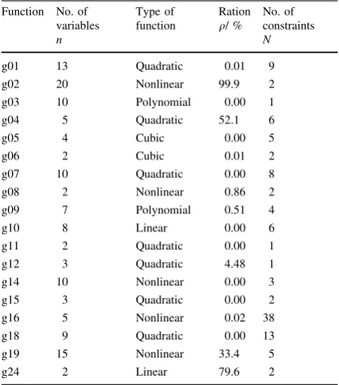
In this part, the performance of the proposed algorithm is verified by 18 benchmark functions from the IEEE CEC2006 [29]. The details of these test functions are listed in Table1. In this table, q=F/S is the estimated ratio between the feasible region and whole search space, where F is the number of feasible ones in S =1,000,000 ran-domly generated from search domain [xmin, xmax]. N

de-notes the number constraints.

5.1 Parameter Settings

For the numerical simulations, the following parameter settings are utilized unless some changes are mentioned: population size NP =50, tolerance of equality d =1 910-4, crossover rate CR =0.9, scaling factor F=0.8, maximum generation g=600. Meanwhile, the parameters of the shrinking space technique are set as:

T¼20; b¼pnffiffiffiffiffiffiffiffiffi0:02

;

ai¼ x0max;ixmin;i0

= 203lg

xmax;i0x_min;i0

ð Þ

:

ð20Þ

To compare the robustness of different algorithms, bench-mark functions are optimized at 30 independent runs. Then their statistical performances of the optimal solutions such as mean, standard deviation criteria are utilized to compare.

Perform the improved DE to generate 3NP individuals

Select the best NP individuals from combined population by ATM

Compute ( ), ( ), f x G x ϕ

Reduce the region by shrinking space technique

Output optimal solution mod(g, T)=0

FFEs>max_FFEs Initialization

0 { ,1 , i, , NP} P= x Lx L x

N

Y

Y N

5.2 General Performance of ATMDE

The numerical results of the eighteen-benchmark func-tions obtained by the ATMDE algorithm are summarized in Table2. This table includes the known ‘‘optimal’’ solution for each benchmark function and the ‘‘best’’, ‘‘median’’, ‘‘mean’’, ‘‘worst’’, and ‘‘standard deviation’’ of each test function solved by the ATMDE algorithm. From Table2, it shows that ATMDE has the strong ability to converge to the global optima for all test functions expect for functions g02 and g19. However, the benchmark functions g02 and g19 solved by ATMDE are extremely close to the known ‘‘optimal’’ values with small standard deviations. The rest sixteen test functions (g01, g03, g04, g05, g06, g07, g08, g09, g10, g11, g12, g14, g15, g16, g18, g24) can be found consistently to achieve ‘‘optimal’’ values in terms of the ‘‘best’’, ‘‘me-dian’’, ‘‘mean’’, ‘‘worst’’, and ‘‘standard deviation’’ cri-teria. Especially, the functions g01 and g12 can both converge to ‘‘optimal’’ values and their standard devia-tions are zero, which means that 30 independent runs can obtain their corresponding optimal values.

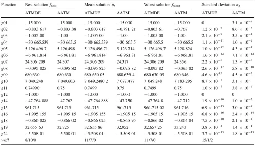
5.3 ATMDE Compared with AATM

The principal aim of this part verifies that the improved DE as the search optimizer is very effective and can be utilized to further enhance the performance of AATM.

To make a fair comparison, the results of benchmark functions by AATM are obtained from the original lit-erature [28]. The comparison results between AATM and ATMDE are listed in Table3. w/t/l denotes that the proposed ATMDE wins in w functions, equals to t functions, and loses in l functions, compared with AATM algorithm. The results by ATMDE is signifi-cantly better than those solved by AATM in 8, 11, 11, and 15 functions in terms of the ‘‘best’’, ‘‘mean’’, ‘‘worst’’, and ‘‘standard deviation’’ criteria, respectively. It equals to its corresponding results in 10, 7, 7, and 1 functions from the above criteria. For the standard deviations, the results only lose in functions g08 and g24, but their differences are extremely close and they both can achieve the ‘‘optimal’’ results with exceedingly small standard deviation. Based on the above compar-ison, it is clear that ATMDE achieves the competitive better performance than AATM in terms of the quality of the results by these benchmark functions.

Furthermore, the computational cost of ATMDE and AATM both are relatively low compared with the IS-PAES algorithm [27], but the performance of ATMDE is better than those solved by AATM in terms of quality of results. It should be noted that comparison results between AATM and IS-PAES are shown in the reference [28] in which AATM with smaller fitness function evaluations (FFEs) has better performance than IS-PAES. Hence, ATMDE is an effective and efficient algorithm with limited FFEs for solving COPs.

5.4 Effectiveness of the ‘‘DE/rand/best/1’’ Strategy

In order to verify the effectiveness of the proposed ‘‘DE/ rand/best/1’’ strategy, 18 test functions are also employed to perform another numerical simulation (i.e. ATMDE1) which only ‘‘DE/rand/1’’ without ‘‘DE/best/1’’ strategy is used to generate the first offspring y₁in the whole search process. For each function, 30 independent runs are also conducted without changing any parameter settings. The comparing results of ATMDE and ATMDE1 summarizes in Table4. Eleven functions (i.e. g04, g05, g06, g08, g09, g11, g12, g14, g15, g18, g24) can consistently converge to the global optima solved by both ATMDE and ATMDE1. However, the results of the seven functions (i.e. g01, g02, g03, g07, g10, g16, g19) solved by ATMDE can achieve the global optima but the ATMDE1 cannot consistently obtain ones especially for the functions g02, g03 and g10. More specifically, the results achieved by ATMDE are better than those solved by ATMDE1 in 6, 6, 7, 7 and 14 functions in terms of the ‘‘best’’, ‘‘median’’, ‘‘mean’’, ‘‘worst’’, and ‘‘standard deviation’’ criteria, respectively. It ties its corresponding results in 12, 12, 11, 11 and 3 functions from the above criteria. For the standard Table 1 Details about 18 benchmark functions

Function No. of variables

n

Type of function

Ration

q/ %

No. of constraints

N

g01 13 Quadratic 0.01 9

g02 20 Nonlinear 99.9 2

g03 10 Polynomial 0.00 1

g04 5 Quadratic 52.1 6

g05 4 Cubic 0.00 5

g06 2 Cubic 0.01 2

g07 10 Quadratic 0.00 8

g08 2 Nonlinear 0.86 2

g09 7 Polynomial 0.51 4

g10 8 Linear 0.00 6

g11 2 Quadratic 0.00 1

g12 3 Quadratic 4.48 1

g14 10 Nonlinear 0.00 3

g15 3 Quadratic 0.00 2

g16 5 Nonlinear 0.02 38

g18 9 Quadratic 0.00 13

g19 15 Nonlinear 33.4 5

deviation criterion, the function g11 solved by ATMDE1 is smaller than one by ATMDE, but they both can obtain the optimal result with an exceedingly small difference. Based

on the above analysis, the proposed ‘‘DE/rand/best/1’’ strategy is a very important part of the proposed ATMDE algorithm.

Table 2 Results obtained by ATMDE for 18 benchmark test function over 30 independent runs

Function Optimal solution

f*

Best solution

fbest

Median solution

fmedian

Mean solution

lf

Worst solution

fworst

Standard deviation

rf

g01 -15.000 -15.000 -15.000 -15.000 -15.000 0

g02 -0.803 619 -0.803 617 -0.803 617 -0.803 617 -0.803 610 1.238 9910-6

g03 -1.000 50 -1.005 00 -1.005 00 -1.005 00 -1.005 00 2.081 6910-9

g04 -30 665.538 6 -30 665.538 6 -30 665.538 6 -30 665.538 6 -30 665.538 6 1.110910-11

g05 5126.496 71 5126.496 71 5126.496 71 5126.496 71 5126.496 71 1.013 3910-12

g06 -6961.813 87 -6961.813 87 -6961.813 87 -6961.813 87 -6961.813 87 1.850910-12

g07 24.306 209 24.306 209 24.306 209 24.306 209 24.306 209 2.211 4910-8

g08 -0.095 825 -0.095 825 -0.095 825 -0.095 825 -0.095 825 2.564 1910-17

g09 680.630 05 680.630 05 680.630 05 680.630 05 680.630 05 4.634 8910-13

g10 7049.248 02 7049.248 02 7049.248 02 7049.248 02 7049.24802 8.700910-7

g11 0.749 90 0.749 90 0.749 90 0.749 90 0.749 90 1.011 2910-7

g12 -1.000 00 -1.000 00 -1.000 00 -1.000 00 -1.000 00 0

g14 -47.764 888 -47.764 888 -47.764 888 -47.764 888 -47.764 888 1.953 9910-10

g15 961.715 022 961.715 022 961.715 022 961.715 022 961.715 022 6.937 8910-13

g16 -1.905 155 -1.905 155 -1.905 155 -1.905 155 -1.905 155 6.775 2910-16

g18 -0.866 025 -0.866 025 -0.866 025 -0.866 025 -0.866 025 7.454 9910-10

g19 32.655 59 32.655 63 32.655 86 32.656 00 32.657 25 3.753 8910-4

g24 -5.508 013 -5.508 013 -5.508 013 -5.508 013 -5.508 013 3.735 5910-15

Table 3 Comparison results of ATMDE and AATM on 18 benchmark test functions

Function Best solutionfbest Mean solutionlf Worst solutionfworst Standard deviationrf

ATMDE AATM ATMDE AATM ATMDE AATM ATMDE AATM

g01 -15.000 -15.000 -15.000 -15.000 -15.000 -15.000 0 3.1910-7

g02 -0.803 617 -0.803 38 -0.803 617 -0.791 21 -0.803 61 -0.767 1.2910-6 8.6910-3

g03 -1.005 00 -1.00 -1.005 00 -1.00 -1.005 00 -1.00 2.1910-9 3.5910-4

g04 -30 665.539 -30 665.5 -30 665.539 -30 665.5 -30 665.5 -30 665.5 1.1910-11 _1.0910-4

g05 5 126.496 7 5 126.498 5 126.496 71 5 126.714 5 126.496 7 5 128.824 1.0910-12 4.3910-1

g06 -6 961.814 -6 961.81 -6 961.814 -6 961.81 -6 961.81 -6 961.81 1.6910-12 7.1910-12

g07 24.306 209 24.307 24.306 209 24.317 24.306 209 24.356 2.2910-8 1.3910-2

g08 -0.095 825 -0.095 82 -0.095 825 -0.095 82 -0.095 82 -0.095 82 2.6910-17 5.8910-18

g09 680.630 680.630 680.630 05 680.639 4 680.630 05 680.646 4.6910-13 4.5910-3

g10 7 049.248 7 049.603 7 049.2480 2 7 077.477 7 049.248 7 183.295 8.7910-7 3.19101

g11 0.74990 0.75 0.7499 0.75 0.7499 0.75 1.0910-7 _3.8910-6

g12 -1.000 -1.000 -1.000 -1.000 -1.000 -1.000 0 0

g14 -47.764 888 -47.762 -47.764 888 -47.750 -47.764 8 -47.712 1.9910-10 1.0910-2

g15 961.715 961.715 961.715 961.715 961.715 02 961.716 6.9910-13 3.0910-4

g16 -1.905 155 -1.905 15 -1.905 155 -1.905 15 -1.905 15 -1.905 15 6.8910-16 2.4910-14

g18 -0.866 025 -0.866 02 -0.866 025 -0.865 95 -0.866 02 -0.864 84 7.5910-10 2.1910-4

g19 32.655 63 32.725 32.655 86 32.952 32.657 25 33.243 3.8910-4 1.4910-1

g24 -5.508 01 -5.508 01 -5.508 01 -5.508 01 -5.508 01 -5.508 01 3.7910-15 1.8910-15

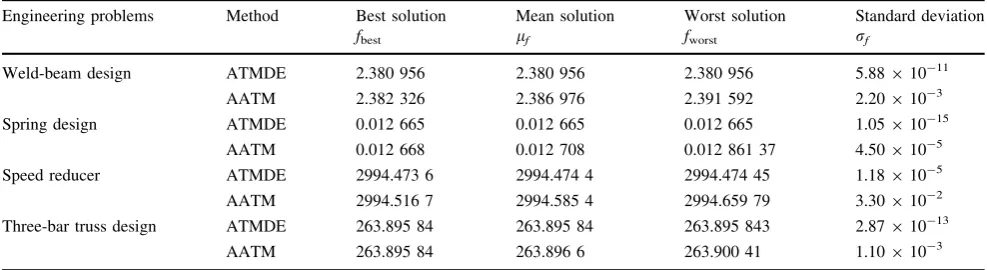
5.5 Four Mechanical Benchmark Engineering Designs

The four mechanical benchmark engineering problems are used by many researchers to demonstrate the performance of different algorithms. Different characteristics of objec-tive functions and constraints are illustrated as shown in Table5. The four mechanical engineering designs [28] are the minimum cost of a weld-beam design, the minimum

weight of a spring design, the minimum weight of a speed reducer design and the minimum volume of a three-bar truss design, respectively. Table6 summarizes the com-parative results of these problems solved by ATMDE and AATM in terms of the ‘‘best’’, ‘‘mean’’, ‘‘worst’’, and ‘‘standard deviation’’ metrics. It shows that the ATMDE has the better statistically quality and robustness than AATM under the same number of function fitness evalu-ations in terms of the selected performance criteria. Table 4 Results obtained by ATMDE and ATMDE1 on 18 benchmark test functions

Function Method Best solution

fbest

Median solution

fmedian

Mean solution

lf

Worst solution

fworst

Standard deviation

rf

g01 ATMDE -15.000 -15.000 -15.000 -15.0000 0

ATMDE1 -14.999 9 -14.999 9 -14.999 9 -14.999 9 8.98910-7

g02 ATMDE -0.803 617 -0.803 617 -0.803 617 -0.803 610 1.24910-6

ATMDE1 -0.802 125 -0.802 125 -0.802 124 -0.802 092 6.14910-6

g03 ATMDE -1.005 00 -1.005 00 -1.005 00 -1.005 00 2.08910-9

ATMDE1 -1.005 00 -1.005 00 -0.985 8 -0.798 4 4.93910-2

g04 ATMDE -30 665.53 -30 665.53 -30 665.53 -30 665.5 1.11910-11

ATMDE1 -30 665.53 -30 665.53 -30 665.53 -30 665.53 1.85910-11

g05 ATMDE 5126.496 71 5 126.496 71 5126.496 71 5 126.496 71 1.01910-12

ATMDE1 5126.496 71 5 126.496 71 5126.496 71 5 126.496 71 2.95910-9

g06 ATMDE -6961.813 -6961.813 -6961.813 -6961.81 1.85910-12

ATMDE1 -6961.813 -6961.813 -6961.813 -6961.81 2.78910-12

g07 ATMDE 24.306 209 24.306 209 24.306 209 24.306 209 2.21910-8

ATMDE1 24.3062 497 24.306 2497 24.306 253 24.306 364 2.09910-5

g08 ATMDE -0.095 825 -0.095 825 -0.095 825 -0.095 825 2.56910-17

ATMDE1 -0.095 825 -0.095 825 -0.095 825 -0.095 825 2.82910-17

g09 ATMDE 680.630 05 680.630 05 680.630 05 680.630 05 4.63910-13

ATMDE1 680.630 05 680.630 05 680.630 05 680.630 05 4.85910-13

g10 ATMDE 7 049.248 02 7 049.248 02 7 049.248 02 7 049.248 02 8.70910-7

ATMDE1 7 049.339 29 7 049.699 7 7 049.800 6 7 051.246 3 4.59910-1

g11 ATMDE 0.749 90 0.749 90 0.749 90 0.749 90 1.01910-7

ATMDE1 0.749 90 0.749 90 0.749 90 0.749 90 1.12910-16

g12 ATMDE -1.000 00 -1.000 00 -1.000 00 -1.000 00 0

ATMDE1 -1.000 00 -1.000 00 -1.000 00 -1.000 00 0

g14 ATMDE -47.764 888 -47.764 888 -47.764 888 -47.764 88 1.95910-10

ATMDE1 -47.764 888 -47.764 888 -47.764 888 -47.764 88 1.67910-8

g15 ATMDE 961.715 022 961.715 022 961.715 022 961.715 022 6.94910-13

ATMDE1 961.715 022 961.715 022 961.715 022 961.715 022 6.94E910-13

g16 ATMDE -1.905 155 -1.905 155 -1.905 155 -1.905 155 6.78910-16

ATMDE1 -1.905 102 -1.905 102 -1.905 102 -1.905 102 6.78910-16

g18 ATMDE -0.866 025 -0.866 025 -0.866 025 -0.866 025 7.45910-10

ATMDE1 -0.866 025 -0.866 025 -0.866 025 -0.866 025 4.49910-6

g19 ATMDE 32.655 63 32.655 86 32.656 00 32.657 25 3.75910-4

ATMDE1 32.676 38 32.702 88 32.704 75 32.774 96 2.16910-2

g24 ATMDE -5.508 013 -5.508 013 -5.508 013 -5.508 013 3.74910-15

ATMDE1 -5.508 013 -5.508 013 -5.508 013 -5.508 013 4.52910-15

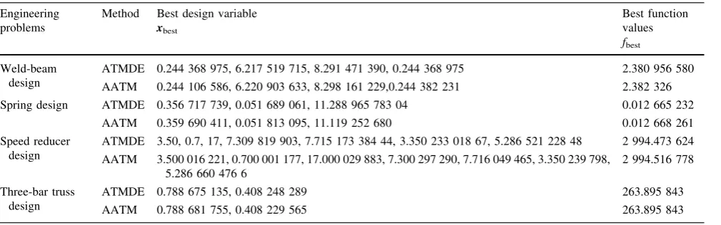
Moreover, the four standard deviations obtained by ATMDE are relatively small, which is a crucial feature for application of the approach for solving the practical world problems. Table7 lists the best design variables obtained by ATMDE and AATM for four engineering design problems associated with their corresponding optimal results, which show the ATMDE algorithm can obtain better solution than the AATM.

6 Engineering Applications

6.1 Vehicle Crashworthiness Problem

In the automotive industry, structural optimization design for vehicle crashworthiness has become a paramount research field. In this paper, different characteristics of low- and high-speed crashworthiness are considered simultaneously [30]. For the frontal impact, the most cru-cial energy absorbing components including rail, collision beam and stiffener can directly affect the performance of vehicle crashworthiness and safety. Therefore, the total mass M(x) of selected parts including collision beam, stiffener, front rail and front rail cover as shown in Fig.4is considered as our optimization objective and it is also subjected to acceleration, energy-absorbing and maximum intrusion constraints. Then, the crashworthiness problem could be formulated as

minfðxÞ ¼MðxÞ;

s:t:

g1ðxÞ ¼aðxÞ 350;

g2ðxÞ ¼EðxÞ 3000;

g3ðxÞ ¼IupðxÞ 3500;

g4ðxÞ ¼IdownðxÞ 2000;

8 > > < > > :

ð21Þ

where x =[x1,x2,x3,x4,x5], 2 mmBx1B3 mm,

1 mmBx2,x3B 2.5 mm, 1.5 mmBx4,x5B 3 mm, aðxÞ

is the mean value of integral acceleration, E(x) is the energy-absorbing of inner and outer front rail, Iup(x) and

Idown(x) are the intrusion of the two points at the engine as

shown in Fig. 5, respectively.

The finite element model (FEM) of the vehicle including 755 parts and 977 742 elements is established for the above objective and constraints. To improve efficiency, the response surfaces are established based on the samples by Latin hypercube sampling method. Then, the minimum massM(x) solved by ATMDE algorithm is 10.53 kg and its corresponding five design variables are 2.00 mm, 2.50 mm, 2.50 mm, 2.76 mm and 1.68 mm, respectively. Under this circumstance, values of constraints are 0 g,

-4208.33 J, -60.74 mm, -0.0002 mm, respectively.

Specifically, the mean value of integral accelerationaðxÞis 35 g, which can effectively protect passengers in the automobile when the collision inevitably occurs. Mean-while, the inner and outer front rail can absorb 3908.33 J. In addition, the intrusions of upper and lower point at the engine are 289.26 mm and 200 mm, which can effectively reduce the occupants’ injuries to protect the passengers’ safety.

6.2 Structural Optimization Design of Tablet Computer

Currently, Tablet computer is one of typical popular con-sumer electronic devices, which have high-integrated density and large power dissipation. It is inevitably for its structural design to consider various aspects of design requirements, such as appearance, portability, operating Table 5 Main features for each engineering design problem

Engineering benchmark No. of variables

n

Ration

q/ %

No. of constrains

N

Weld-beam design 4 37.625 5

Spring design 3 0.732 3 4

Speed reducer design 7 23.015 2 11

Three-bar truss design 2 21.870 6 3

Table 6 Results about four benchmark engineering design problems

Engineering problems Method Best solution

fbest

Mean solution

lf

Worst solution

fworst

Standard deviation

rf

Weld-beam design ATMDE 2.380 956 2.380 956 2.380 956 5.88910-11

AATM 2.382 326 2.386 976 2.391 592 2.20910-3

Spring design ATMDE 0.012 665 0.012 665 0.012 665 1.05910-15

AATM 0.012 668 0.012 708 0.012 861 37 4.50910-5

Speed reducer ATMDE 2994.473 6 2994.474 4 2994.474 45 1.18910-5

AATM 2994.516 7 2994.585 4 2994.659 79 3.30910-2

Three-bar truss design ATMDE 263.895 84 263.895 84 263.895 843 2.87910-13

safety, etc. Hence, structural optimization design of tablet computer should be guaranteed to work well under dif-ferent conditions. This subsection considers the structural optimization design of a 7-inches tablet computer, as illustrated in Fig.6 which mainly includes the touch screen, the display, the battery, the mainboard, the inner bracket, the front shell and the back shell [31]. Our opti-mization objective mainly considers the miniopti-mization of tablet’s thickness D(x). The design problem should be satisfied four practical work conditions including high-temperature constraint g1(x), room-temperature constraint

g2(x), and alternating temperature constraintg3(x) and free

fall constraint g4(x). Hence, this optimization problem

could be formulated as minfðxÞ ¼DðxÞ;

s:t:

g1ðxÞ ¼TCHð Þ x 650;

g2ðxÞ ¼TSHð Þ x 400;

g3ðxÞ ¼CBAð Þ x 240;

g4ðxÞ ¼CTSð Þ x 1000;

8 > > < > > :

ð22Þ

whereTCH(x) denotes the temperature of the chip on the main board under the high-temperature (45°C);TSH(x) is the shell surface temperature with a full load under the room temperature (25°C) for an hour continuously work; CBA(x) is the thermal stress of the battery andCTS(x) is the maximal stress of the touch screen under the collision of the 0.5 m-height free fall. The design variables are the thickness of the front shellx1, the thickness of the display

x2, the thickness of the inner bracketx3, the thickness of the

back shellx4, respectively. And their design values should

be restricted to the domains 4 mmBx1B6 mm,

0.5 mmB x2,x3,x4B2 mm.

Four finite element models (FEM) are constructed for the above four performance constraints. To improve efficiency, the four corresponding response surfaces are established based on the given samples. Furthermore, the accuracy of the response surfaces is verified. Then the

ATMDE algorithm is utilized to solve the tablet com-puter optimization problem. The structural thickness of optimized tablet computer is 6.42 mm which is a 31.7% reduction in compared with that of the original design (6.00 mm, 1.20 mm, 1.20 mm, 1.00 mm), and its design variables are 4.00 mm, 0.51 mm, 1.41 mm and 0.50 mm, respectively. Under this circumstance, the temperature of the chip is 62.05°C and the temperature of shell surface is 37.66 °C which can ensure consumer daily-using comfortably. The thermal stress of battery is about Table 7 Best design variables for four benchmark engineering design problems

Engineering problems

Method Best design variable xbest

Best function values

fbest

Weld-beam design

ATMDE 0.244 368 975, 6.217 519 715, 8.291 471 390, 0.244 368 975 2.380 956 580

AATM 0.244 106 586, 6.220 903 633, 8.298 161 229,0.244 382 231 2.382 326

Spring design ATMDE 0.356 717 739, 0.051 689 061, 11.288 965 783 04 0.012 665 232

AATM 0.359 690 411, 0.051 813 095, 11.119 252 680 0.012 668 261

Speed reducer design

ATMDE 3.50, 0.7, 17, 7.309 819 903, 7.715 173 384 44, 3.350 233 018 67, 5.286 521 228 48 2 994.473 624

AATM 3.500 016 221, 0.700 001 177, 17.000 029 883, 7.300 297 290, 7.716 049 465, 3.350 239 798, 5.286 660 476 6

2 994.516 778

Three-bar truss design

ATMDE 0.788 675 135, 0.408 248 289 263.895 843

AATM 0.788 681 755, 0.408 229 565 263.895 843

Fig. 4 Selected design variables

24 MPa, which can make sure the operating safety in daily. The maximal stress of touch screen is about 100 MPa, which can avoid the device broken during the collision of 0.5 m free fall. This optimized structural design is meaningful because the consumers are satisfied with the final design with better the appearance and portability for the tablet.

7 Conclusions

(1) An improved differential evolution with shrinking space technique and adaptive trade-off model, named ATMDE, is proposed to solve constrained optimiza-tion problems with high accuracy and robustness. (2) The new ‘‘DE/rand/best/1’’ mutant strategy is

con-structed to generate offspring by the feasibility proportion of the current population, which could enhance performance of the ATMDE illustrated by results of test functions.

(3) In comparison with AATM algorithm, ATMDE achieves better performance verified by the simula-tion results of eighteen benchmark test funcsimula-tions from the IEEE CEC2006.

(4) The ATMDE is employed to optimize the structural optimization design of tablet computer, and the optimized thickness is a 31.7% reduction in com-pared with that of the original design.

Open Access This article is distributed under the terms of the Creative Commons Attribution 4.0 International License (http://crea tivecommons.org/licenses/by/4.0/), which permits unrestricted use, distribution, and reproduction in any medium, provided you give appropriate credit to the original author(s) and the source, provide a link to the Creative Commons license, and indicate if changes were made.

References

1. HULL P V, TINKER M L, DOZIER G. Evolutionary optimiza-tion of a geometrically refined truss[J].Structural and Multidis-ciplinary Optimization, 2006, 31(4): 311–319.

2. ZHAO Y, CHEN G, WANG H, et al. Optimum selection of mechanism type for heavy manipulators based on particle swarm optimization method[J]. Chinese Journal of Mechanical Engi-neering, 2013, 26(4): 763–770.

3. TANG Q, LI Z, ZHANG L, et al. Effective hybrid teaching-learning-based optimization algorithm for balancing two-sided assembly lines with multiple constraints[J].Chinese Journal of Mechanical Engineering, 2015, 28(5): 1067–1079.

4. WANG Y, LIU H, CAI Z, et al. An orthogonal design based constrained evolutionary optimization algorithm[J].Engineering Optimization, 2007, 39(6): 715–736.

5. WANG L, LI L. An effective differential evolution with level comparison for constrained engineering design[J].Structural and Multidisciplinary Optimization, 2010, 41(6): 947–963.

6. CHEN D N, ZHANG R X, YAO C Y, et al. Dynamic topology multi force particle swarm optimization algorithm[J]. Chinese Journal of Mechanical Engineering, 2016, 29(1): 124–135. 7. RAO R, SAVSANI V, BALIC J. Teaching-learning-based

opti-mization algorithm for unconstrained and constrained real-pa-rameter optimization problems[J]. Engineering Optimization, 2012, 44(12): 1447–1462.

8. QUARANTA G, FIORE A, MARANO G C. Optimum design of prestressed concrete beams using constrained differential evolu-tion algorithm[J].Structural and Multidisciplinary Optimization, 2014, 49(3): 441–453.

9. ZHAO Y, WANG H, WANG W, et al. New hybrid parallel algorithm for variable-sized batch splitting scheduling with alternative machines in job shops[J]. Chinese Journal of Mechanical Engineering, 2010, 23(4): 484–495.

10. COELLO C A C. Theoretical and numerical constraint-handling techniques used with evolutionary algorithms: a survey of the state of the art[J].Computer Methods in Applied Mechanics and Engineering, 2002, 191(11): 1245–1287.

11. TESSEMA B, YEN G G. An adaptive penalty formulation for constrained evolutionary optimization[J].IEEE Transactions on Systems, Man and Cybernetics, Part A: Systems and Humans,

2009, 39(3): 565–578.

12. DEB K, DATTA R. A bi-objective constrained optimization algorithm using a hybrid evolutionary and penalty function approach[J].Engineering Optimization, 2013, 45(5): 503–527. 13. DEB K. An efficient constraint handling method for genetic

algorithms[J]. Computer Methods in Applied Mechanics and Engineering, 2000, 186(2): 311–338.

14. BALAMURUGAN R, RAMAKRISHNAN C, SWAMI-NATHAN N. A two phase approach based on skeleton conver-gence and geometric variables for topology optimization using genetic algorithm[J].Structural and Multidisciplinary Optimiza-tion, 2011, 43(3): 381–404.

15. Venkatraman S, YEN G G. A generic framework for constrained optimization using genetic algorithms[J].IEEE Transactions on Evolutionary Computation,2005, 9(4): 424–435.

16. JIAO L, LI L, SHANG R, et al. A novel selection evolutionary strategy for constrained optimization[J]. Information Sciences, 2013, 239: 122–141.

17. STORN R, PRICE K. Differential evolution–a simple and effi-cient heuristic for global optimization over continuous spaces[J].

Journal of Global Optimization, 1997, 11(4): 341–359. 18. STORN R. System design by constraint adaptation and

differ-ential evolution[J].IEEE Transactions on Evolutionary Compu-tation,1999, 3(1): 22–34.

19. LANDA B R, COELLO C A C. Cultured differential evolution for constrained optimization[J]. Computer Methods in Applied Mechanics and Engineering, 2006, 195(33): 4303–4322. 20. MEZURA-MONTES E, COELLO C A C, VEL Z J, et al.

Mul-tiple trial vectors in differential evolution for engineering design[J].Engineering Optimization, 2007, 39(5): 567–589. 21. ZHANG M, LUO W, WANG X. Differential evolution with

dynamic stochastic selection for constrained optimization[J]. In-formation Sciences, 2008, 178(15): 3043–3074.

22. MALLIPEDDI R, SUGANTHAN P N. Ensemble of constraint handling techniques[J]. IEEE Transactions on Evolutionary Computation,2010,14(4): 561–579.

23. ELSAYED S M, SARKER R A, ESSAM D L. Multi-operator based evolutionary algorithms for solving constrained optimiza-tion problems[J]. Computers & Operations Research, 2011, 38(12): 1877–1896.

24. GONG W, CAI Z, LIANG D. Engineering optimization by means of an improved constrained differential evolution[J]. Computer Methods in Applied Mechanics and Engineering, 2014, 268: 884–904.

25. WANG C, FANG Y, GUO S. Multi-objective optimization of a parallel ankle rehabilitation robot using modified differential evolution algorithm[J]. Chinese Journal of Mechanical Engi-neering, 2015, 28(4): 702–715.

26. WANG Y, CAI Z, ZHOU Y, et al. An adaptive tradeoff model for constrained evolutionary optimization[J].IEEE Transactions on Evolutionary Computation,2008, 12(1): 80–92.

27. AGUIRRE A H, RIONDA S B, COELLO C A C, et al. Handling constraints using multiobjective optimization concepts[J]. Inter-national Journal for Numerical Methods in Engineering, 2004, 59(15): 1989–2017.

28. WANG Y, CAI Z, ZHOU Y. Accelerating adaptive trade-off model using shrinking space technique for constrained evolu-tionary optimization[J]. International Journal for Numerical Methods in Engineering, 2009, 77(11): 1501–1534.

29. LIANG J J, RUNARSSON T, MEZURA-MONTES E, et al. Problem definitions and evaluation criteria for the CEC 2006 special session on constrained real-parameter optimization[R].

Technical report, Nanyang Technological University, Singapore. 2006.

30. JIANG C, DENG S L. Multi-objective optimization and design considering automotive high-speed and low-speed crashworthi-ness[J]. Chinese Journal of Computational Mechanics, 2014, 31(4): 474–479. (in Chinese)

31. HUANG Z, JIANG C, ZHOU Y, et al. Reliability-based design optimization for problems with interval distribution parame-ters[J]. Structural and Multidisciplinary Optimization, 2016, 1–16, doi:10.1007/s00158-016-1505-3.

Chunmming FU,born in 1987, is currently a PhD candidate atState Key Laboratory of Advanced Design and Manufacturing for Vehicle Body, Hunan University, China. His research interests include structural optimization design, differential evolution and constrained optimization. E-mail: [email protected]

Yadong XU, born in 1978, is currently an associate professor at

Nanjing University of Science and Technology, China. His research interests include structural optimization design and composite mate-rial. E-mail: [email protected]

Chao JIANG, born in 1978, is currently a professor and PhD candidate supervisor at Hunan University, China. His research interests include mechanical design, uncertainty analysis and relia-bility. Tel:?86-731-88821748; E-mail: [email protected]

Xu HAN,born in 1968, is currently a professor and a PhD candidate supervisor atHunan University, China. His research interests include mechanical design, uncertainty analysis and reliability. E-mail: [email protected]