On the Importance of
the Artificial Bee Colony
Control Parameter ‘Limit’
ITC 4/46Journal of Information Technology and Control
Vol. 46 / No. 4 / 2017 pp. 566-604
DOI 10.5755/j01.itc.46.4.18215 © Kaunas University of Technology
On the Importance of the Artificial Bee Colony Control Parameter ‘Limit’
Received 2017/05/21 Accepted after revision 2017/10/23
http://dx.doi.org/10.5755/j01.itc.46.4.18215
Corresponding author: [email protected]
Niki Veček
University of Maribor, Faculty of Electrical Engineering and Computer Science, Koroška cesta 46, 2000 Maribor, Slovenia, e-mail: [email protected]
Shih-Hsi Liu
California State University, Fresno, Department of Computer Science, 2576 E San Ramon Ave., Fresno, CA, USA, e-mail: [email protected]
Matej Črepinšek, Marjan Mernik
University of Maribor, Faculty of Electrical Engineering and Computer Science, Koroška cesta 46, 2000 Maribor, Slovenia, e-mail: [email protected], [email protected]
Artificial Bee Colony (ABC) is a successful meta-heuristic algorithm that has been greatly utilised by research-ers. Through our practical experience of ABC, we have noticed that the recommended formula ‘limit’ = ne * D
may not be the best choice for different problems. In this work, a set of experiments using horizontal and ver-tical approaches has been designed and executed with the aim of observing the effect of ‘limit’ on ABC. The results have been statistical analysed using Null Hypothesis Significance Testing (NHST) as well as the Chess Rating System for Evolutionary Algorithms (CRS4EAs), which is a novel approach for comparing meta-heu-ristic algorithms. It is shown that the recommended formula is not the best setting for different problems and approaches. Hence, the control parameter ‘limit’ should be tuned or controlled. The other important result of this study is to show that CRS4EAs is comparable but also shows benefits over NHST.
1. Introduction
Comparisons between different meta-heuristic algo-rithms [5] are inevitably necessary within the field of Evolutionary Computation (EC). Although the scientific testing [20] approach, the aim of which is to learn about which kinds of problems and why one algorithm performs better, is preferred over the horse racing approach [12], [23], [45], the aim of which is to outperform other algorithms, the latter approach still prevails during current EC experimental practices. However, even in the scientific testing approach, sim-ply understanding parameter interactions and plac-ing emphasis on the analysis of robustness may not be enough if an algorithm under investigation performs badly. Hence, there is still a need for comparing the performances of the algorithms under investigation using the currently best available algorithms [9]. This paper deals with the Artificial Bee Colony (ABC) algorithm [25], [26], [39], which is a swarm intel-ligence algorithm that accomplishes optimisation tasks through social cooperation among bees (i.e., individuals) – employed bees exploit food source and share food source information to onlooker bees; on-looker bees probabilistically choose and exploit food source based on the provided information; and scout bees explore new food source when current ones are exhausted. ABC exhibits remarkable balance between exploitation and exploration [8] (raw data for exper-iments presented in this paper are available in [47]). This balance between exploitation (employed bee phase and onlooker bee phase) and exploration (scout bee phase) is controlled by population size (SN) and ‘limit’, respectively. The formula ‘limit’ = ne * D
(‘lim-it’ is the threshold for determining whether a scout bee should be introduced or not, ne is the number of
employed bees, D is the dimension of a problem) was recommended in a very influential paper [26]. As ABC is a very successful algorithm, it has been used extensively over recent years [28], [29]. The suggest-ed formula for setting the ‘limit’ control parameter is indeed mostly used (e.g., [2]). We came across only a few studies where the ‘limit’ was set at a certain fixed number (e.g., 10 in [38], [55], 30 in [53], 40 in [56], 50 in [44], 100 in [22], [52], 200 in [34], [57]), or better where the ‘limit’ was tuned [35]. When experimenting using ABC we have noticed its sensitiveness to ‘limit’ control parameter and that its relationship between
population size (SN = 2 * ne) and the dimension of a
problem (D) is not straightforward. However, this was just our speculation driven by practical experience with ABC. Hence, we decided to perform extensive statistical analysis of ABC and support it by stronger conclusions, using the Null Hypothesis Significance Testing (NHST) [41] and Chess Rating System for Evolutionary Algorithms (CRS4EAs) [48]. For find-ing the significant differences with NHST, the Wil-coxon’s test [51] was a more appropriate test with the post-hoc analysis supported by the Holm’s test [19]. Both the Wilcoxon’s test and CRS4EAs compare the results pairwisely but whilst the Wilcoxon’s compar-ison concentrates only on 1×k comparison, the com-parison in CRS4EAs allows k×k comparison and the detections of significant differences amongst all algo-rithms. Note that when attempting to apply statistical
k×k comparison, the more appropriate test would be the Friedman test [13], [14]. However, as the number of problems is really small and the goal was to anal-yse different ‘limit’ settings regarding different prob-lems, the Friedman test could not be taken into con-sideration [50]. Hence, the choice of Wilcoxon’s test with post-hoc Holm’s test is shown as an appropriate one. Even though CRS4EAs allows k×k comparison and Wilcoxon’s test allows only 1×k comparison, the analysis of CRS4EAs was applied as 1×k comparison, as well as assuring that both methods are applied equally. Our results show that ABC’s performance is very sensitive to a control parameter ‘limit’, which is often independent regarding the population size. Whilst the ‘limit’ depends on dimension D, it is much more dependent on the problem under investigation. Although, the characteristics of a problem might drastically change when changing dimension D and can become a completely different problem (e.g., an optimisation function becomes multi-modal instead of uni-modal or vice verse, and the fitness-distance correlation is changed from high to low correlation or vice verse [7]). Hence, dimension D can be seen as part of a problem as well.
The main contributions of this paper are:
_ Sensitivity analysis is applied for the first time
parameter ‘limit’, which must be carefully set for the best results;
_ An example of how from sensitivity analysis
one might conclude that a suggested formula for setting control parameters is not most appropriate; Deep statistical investigations about setting ABC control parameter ‘limit’ as a full factorial design using NHST and CRS4EAs showing that the recommended formula for setting the control parameter ‘limit’ regarding population size SN and the dimension of the problem D is not the best for every problem and approach;
_ For the first time, it is shown that even the
control parameter ‘limit’ depends on the available maximum number of fitness evaluations, and that ABC convergence using the suggested formula is not amongst the fastest; and
_ First application of CRS4EAs as 1×k comparison
showing its applicability and suitability as a feasible replacement of NHST.
The main conclusion from this study is that ABC does not always perform best when under the setting ‘lim-it’ = ne * D. Hence, the ‘limit’ control parameter should
be tuned or controlled.
However, such a conclusion should not come as a sur-prise in EC and confirms already established knowl-edge within the meta-heuristic field. Namely, fixed formulae for setting a control parameter usually lead to poor performances when applying to different problems. However, a systematic mapping study from [39] shows that this formula is indeed very frequent-ly used indicating that still many researchers believe that some fixed formulae can be a robust choice. Our speculation is that this dichotomy between theory and practice exists due to lack of ABC studies show-ing that such a parameter settshow-ing is not the best. In this respect, our work can be seen as remedying this situation for ABC. There should be no excuse not to perform tuning on control parameter ‘limit’ anymore. The other important conclusion from this study is that CRS4EAs is comparable with NHST but CRS4EAs also showed many benefits during exper-imentation where a greater number of experiments needed to be conducted. When executing one tourna-ment in CRS4EAs, all the necessary data for analysis are obtained and calculated, whilst for NHST there are always additional tests required. Having so many
different situations and approaches, the results anal-ysed by CRS4EAs are far quicker and easier than with NHST.
The paper is organized as follows. Section 2 describes the conducted experiment in detail. This section is divided into three major parts: in Section 2.1 the sen-sitivity analysis is conducted for one optimisation problem; in Section 2.2 the results of experiment are analysed with NHST and the results reported regard-ing the different approaches; in Section 2.3 the results of the experiment are analysed with CRS4EAs and results are again reported regarding the different ap-proaches. Section 3 displays the results of tuning the parameters of ABC on different dimensionalities of one optimisation problem. Section 4 discusses other similar researches as presented in the past. Lastly, Section 5 concludes the paper. All the algorithms, fig-ures and tables are also placed online at https://lpm. feri.um.si/research/abc/.
2. Experiment
The amount of exploration [8] of ABC is controlled by the control parameter ‘limit’. ABC is exploring the search space more often when the ‘limit’ is set at a small number, and vice versa by exploiting the search space when the ‘limit’ is set to a higher number (Algorithm 1). The amount of exploration and exploitation depends on the problem and even on the evolution stage [8]. Hence, it is difficult to quantify. The formula ‘limit’ =
ne * D [26] suggests that higher-dimensional problems
require less exploration (higher dimension increases ‘limit’, which in turn decreases exploration), and that bigger population size increases exploitation, which is indeed correct for ABC. However, the relationship between population size and the needed amount of ex-ploration is unclear, as well as the fact that higher-di-mensional problems might require more exploration. Overall, the suggested formula was not intuitive for us and we decided to further explore the relationships be-tween population size SN (SN = 2 * ne), dimension D,
and control parameter ‘limit’. Our experiment was di-vided into two parts. In the first part, the importance of
emphasis was given to the ABC control parameter ‘lim-it’, where different settings were statistically analysed by NHST and CRS4EAs.
During the experiment, we used the same benchmark functions as in the original ABC work [26]. Although this benchmark suite contained only five numerical benchmark functions: (1) multi-modal, non-sepa-rable Schaffer function f1, (2) uni-modal, separable
Sphere function f2, (3) multi-modal, non-separable
Griewank function f3, (4) multi-modal, separable
Rastrigin function f4, and (5) uni-modal,
non-sepa-rable Rosenbrock function f5, it was enough to arrive
at appropriate conclusions. Even this small bench-mark suite confirmed our hypothesis and there was no need to perform the experiment on more compre-hensive benchmarks. On the other hand, whenever a statistical formula is suggested, it should be tested on comprehensive sets of benchmarks that can really support it on a vast number of different optimisation problems. For example, Piotrowski in [43] suggested that both the problems, minimisation and maximisa-tion should be used on the same benchmark funcmaximisa-tions since a good performance of a meta-heuristic algo-rithm on the minimisation of some function does not also guarantee a good performance on the maximisa-tion of the same funcmaximisa-tion, and vice versa.
We extended Karaboga’s experiment [26] by perform-ing a full factorial design on this benchmark suite usperform-ing the following factors and their values: SN = {24, 50, 100},
D = {2, 5, 10, 30, 50}, and ‘limit’ = {0, 100, 250, 500, 750, 1000, 1250, 1500, ∞}. Hence, altogether there were 3 * 5 * 9 = 135 different combinations tested using 100 inde-pendent runs, whilst using both vertical and horizontal approaches [18] when performing the experiments. In the first case, known also as ‘the fixed-cost approach’, we measured the quality of a solution reached by a pre-defined number of fitness evaluations (100,000 and 250,000 fitness evaluations for each combination). In the second case, also known as ‘the fixed-target ap-proach’, we measured the number of fitness evalua-tions needed to find a (sub-)optimal solution (10-6 and
10-12). The horizontal approach would have stopped
the algorithm if a (sub-)optimal solution could not be found over 1,000,000 fitness evaluations.
2.1. Sensitivity Analysis
In this subsection, the results of the first part of the experiment are presented showing the importance of
SN, D, and ‘limit’ to the performance of ABC.
Sensitiv-ity analysis [33] is shown only for f1 due to its
similar-ity of results on f2 – f5. The other reason is that the
em-phasis of this study was given to the second part of the experiment, where different settings of ‘limit’ were statistically analysed, and in the third part where the results were analysed using a novel method for pair-wise comparison, CRS4EAs.
The aim of sensitivity analysis was to show the ro-bustness of a meta-heuristic algorithm against dif-ferent settings of control parameters. By performing a sensitivity analysis, we could find those control parameters (if any) that are very sensitive, as well of those (if any) which are very robust. In the former case, a proper setting of a control parameter is crucial for obtaining good performance of a meta-heuristic algorithm, whilst in the latter case, similar perfor-mance can be achieved regardless of the different settings of such non-sensitive control parameters. An obvious question may arise as to why the dimension-ality of problem D was included within our sensitivi-ty analysis as a factor as it is not a control parameter but D should be considered as part of the optimisation problem? As the formula ‘limit’ = ne * D [26] suggested
a particular correlation between ‘limit’ and two oth-er variables: population size and dimensionality of a problem, such a correlation should probably be indi-cated by sensitivity analysis as well. If at least one of these factors is insensitive, then the suggested formu-la [26] might not capture the reformu-lationships amongst the factors too well. As shown in the continuation, this was indeed the case.
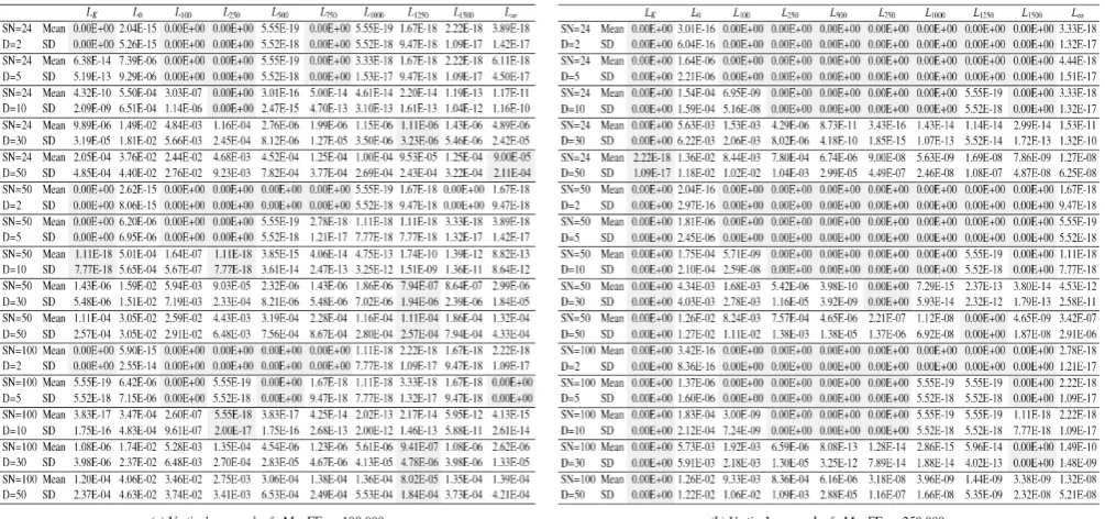
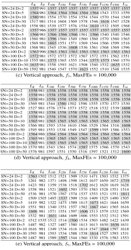
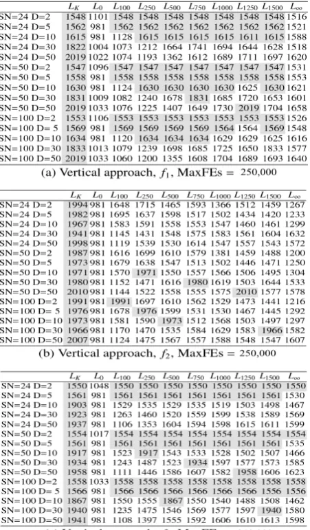
In Tables 1(a) and 1(b), the experimental results of f1
are presented when using the vertical approach with 100,000 and 250,000 maximum number of fitness evaluations (MaxFEs in the tables appeared later), respectively. In Tables 2(a) and 2(b), the experimen-tal results of f1 are presented when using the
horizon-tal approach in order to find a (sub-)optimal solution at 10-6 and at 10-12, respectively. The best results are
highlighted by a light grey colour.
The difference between Tables 1(a) and 1(b)shows that 250,000 fitness evaluations were almost always enough for f1 to find the exact solution; except for high
dimensions D = 30 and D = 50, or when ‘limit’ = 0 (high exploration) and ‘limit’ = ∞ (no exploration). The Karaboga’s setting of ‘limit’ Lk was always the better
Table 1
Mean values (Mean) and standard deviation values (SD) for the vertical approach to problem f1
Table 2
other fixed ‘limit’ values performed better; in most cases (8 out of 15), the better performing value being
L250. A meticulous reader may notice that those
prob-lems with higher dimensions always required more fitness evaluations in order to reach a sub-optimal solution (Tables 2(a) and 2(b)), which was an expect-ed property. Less expectexpect-edly, the population size did not have a big influence on this property. For example, to reach 10-6, the following average numbers of
fit-ness evaluations were needed at L1000: 5.65E+03 (SN =
100, D = 2), 5.60E+03 (SN = 50, D = 2), and 5.31E+03 (SN = 24, D = 2), whilst 8.14E+04 (SN = 100, D = 30), 8.17E+04 (SN = 50, D = 30), and 8.22E+04 (SN = 24, D = 30). In order to reach 10-12, twice as many fitness
eval-uations were roughly needed compared to 10-6. Again,
an increase in the number of fitness evaluations was expected, although the magnitude of the increase was
hard to predict. From these tables, as well as based on the results for f2 to f5 (not shown in this paper), we
no-ticed that setting the ‘limit’ was a difficult task. It can be observed that setting the control parameter ‘lim-it’ using the formula from [26] obtained good results only for the vertical approach with 250,000 fitness evaluations. If only one experiment were applied, the wrong conclusions could be drawn. In other cases, a clear winner was hard to discover (if it existed at all). However, we could not define a rule for setting ‘limit’ based on these results as the statistical significance had not yet been examined.
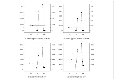
Figure 1shows the sensitivity analyses for the (a) ver-tical approach with a maximum number of 100,000 fitness evaluations; (b) vertical approach with a max-imum number of 250,000 fitness evaluations; (c) hor-izontal approach with (sub-)optimal solution 10-6; (d)
Figure 1
horizontal approach with (sub-)optimal solution 10-12.
The X-axis represents the parameter settings of SN (3 settings: 100, 50, 24 from left to right), D (5 settings: 2, 5, 10, 30, 50 from left to right), and ‘limit’ (9 settings: 0, 100, 250, 500, 750, 1000, 1250, 1500, ∞ from left to right). The Y-axis represents the sensitivities of three parameters in terms of the average of better solutions found and the average number of fitness evaluations needed to reach (sub-)optimal solution amongst 100 runs for vertical and horizontal approaches, respec-tively.
As can be observed, SN had minimal effect. Changing
SN amongst 24, 50, and 100 did not make too much difference. Conversely, ‘limit’ and D played important roles when determining the performance of the ABC algorithm. All the figures indicated that ‘limit’ was more sensitive than D because, in terms of the Y-axis, the range of ‘limit’ was longer than D. Conversely, D is not the ABC control parameter but the property of the problem. Hence, amongst ABC control parameters the size of the population (SN) was much more robust than control parameter ‘limit’, indicating that much more emphasis should be given to properly setting it. All four graphs in Figure 1 show remarkable similar-ities, and although they show that ABC is very sen-sitive to ‘limit’, an important question is: “Are differ-ences in setting ‘limit’ also statistically significant?” Hence, we performed NHST and CRS4EAs analyses on the obtained results. Furthermore, all four graphs in Figure 1clearly indicate that there exists no linear relationship between ‘limit’, population size SN, and dimension D, as suggested by formula [26].
2.2. Null Hypothesis Significance Testing Karaboga’s suggestion of ‘limit’ value Lk = ne*D =
(SN/2)*D [26] was compared to the set of fixed ‘limit’ values ‘limit’ = {0, 100, 250, 500, 750, 1000, 1250, 1500,
Table 3
Description of all four parts of the experiment
∞ } for SN = {24, 50, 100} and D = {2, 5, 10, 30, 50}. The whole experiment was divided into four sections (see Table 3). In the first two sections, we measured the quality of a solution reached by a pre-defined number of fitness evaluations (100,000 and 250,000), which is also known as the vertical or ‘the fixed-cost’ ap-proach. In the other two sections, we measured the number of fitness evaluations needed to find a (sub-) optimal solution (10-6 and 10-12), which is also known
as the horizontal or ‘the fixed-target’ approach. The horizontal approach would have stopped the algo-rithm if a (sub-)optimal solution could not be found over 1,000,000 fitness evaluations. The number of in-dependent runs was in all cases n = 100. By using the vertical approach only the quality of the final solution was taken into consideration but not the convergence. Fast convergence is also a desirable property of me-ta-heuristic algorithms, which can be captured using the horizontal approach. Convergence can also be an-alysed by using the vertical approach and additional Page’s trend statistics, as shown in [10].
The obtained results (readers can find the raw data in [47]) were analysed using Null Hypothesis Signif-icance Testing [41] for multiple comparisons. The non-parametric Wilcoxon’s test [51] was used be-cause the distribution of the data was unknown. In Wilcoxon’s test, the results Lkobtained over n=100
runs for particular settings SN, D and problem fi
were pairwisely compared to the results of another fixed ‘limit’ value obtained over n = 100 runs for the same settings SN, D and problem fi. The differences
between the corresponding outcomes were ranked and the p value was calculated regarding to the sum of positive ranks (whenever Lk was better) and the
sum of negative ranks (whenever Lk was worse). As
several multiple Wilcoxon’s tests were conducted on the same data and we wished to control the Type-I-Error, the post-hoc procedure known as the Holm test [19] was applied to each such comparison. In Holm’s procedure, p values (there is k = 9 of them) obtained using Wilcoxon’s test were ordered from the most sig-nificant (smallest p value, i.e., p1) to the least
signifi-cant (largest p value, i.e., pk). p1 was then compared to
α/(k-1), and if it was smaller, the hypothesis (which states that Lk and ‘limit’ setting linked to p1 are equal)
was rejected. p2 was compared to α/(k -2), p3 to α/(k
-3) and so on, until the value j for which pj was not
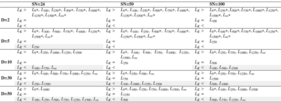
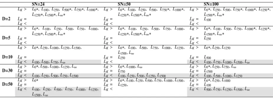
found, the procedure stopped and all the remaining hypotheses were retained. All the results from the presented experiments were analysed under a signif-icance level of α = 0.05. The results of these analyses are presented in Tables 5-21. In each table, Karabo-ga’s ‘limit’ value Lk is compared to other fixed values
of ‘limit’ (L0, L100, L250, L500, L750, L1000, L1250, L1500, L∞). Lk
was either better (>), equal (=), or worse (<) than any fixed value of ‘limit’. The decision whether Lkwas
bet-ter or worse depended on the sums of the positive and negative ranks from the Wilcoxon’s test. Whenever the difference between the two values was significant under the Holm test, there is a star symbol (*) behind the ‘limit’ value. Whenever Karaboga’s ‘limit’ value Lk
was worse than at least one other fixed ‘limit’ value, the cell in the table is highlighted in light grey colour. Since Lk was different for different settings of SN and
D, its values are displayed in Table 4.
Table 4
Values of ‘limit’ Lk= (SN/2)*D
2.2.1. Experiment 1: Vertical Approach with
MaxFEs =100,00
Tables 5-9 show the differences found between Lk
and the other 9 fixed ‘limit’ values on all 5
optimisa-tion problems. While Lk was in most cases better than
some fixed ‘limit’ values, there were some values for which Lk was worse, sometimes even significantly.
In particular, for f1: SN = 24 and D = 5 where Lk was
significantly worse than L100, L250, L500, L750, L1000, L1250,
L1500, L∞; SN = 24 and D = 10 where Lk was
significant-ly worse than L250, L500, L750, L1000, L1250, L1500; SN = 100
and D = 10 where Lk was significantly worse than L250;
SN = 24 and D = 30 where Lk was significantly worse
than L500, L750, L1000, L1250, L1500. For f5: SN = 24 and D =
5 where Lk was significantly worse than L100, L250, L500,
L750, L1000, L1250, L1500, L∞; SN = 50 and D = 5 where Lk was
significantly worse than L500, L750, L1000, L1250, L1500; SN
= 100 and D = 5 where Lk was significantly worse than
L1500; SN = 24 and D = 10 where Lk was significantly
worse than L250, L500, L750, L1000, L1250, L1500, L∞. Hence,
Lk had significantly better alternatives for problems
f1 and f5, whilst for f2, f3, and f4 the found differences
were not significant. The differences between Lk and
some other fixed ‘limit’ values for f1 were significant
when the population size SN equaled 24, and dimen-sion D equaled 5, 10, or 30. So for this problem and small population size, Lk would not be a better choice.
For f5, Lk had significantly better alternatives
whenev-er dimension D equaled 5, and for dimension D = 10 and small population size SN = 24. However, for all five problems, Lk had better alternatives (however,
these alternatives were not significantly better) when dimension D was bigger (10, 30, or 50) and population size SN had different values.
Table 5
Table 6
f2, vertical approach, MaxFEs = 100,000, NHST
Table 7
f3, vertical approach, MaxFEs = 100,000, NHST
Table 8
Table 9
f5, vertical approach, MaxFEs = 100,000, NHST
Table 10
f1, vertical approach, MaxFEs = 250,000, NHST
Table 11
Table 13
f4, vertical approach, MaxFEs = 250,000, NHST
Table 14
f5, vertical approach, MaxFEs = 250,000, NHST Table 12
On the other hand, for f1 and f4, Lk was never the
abso-lute best value, meaning that there was always a better or at least equal ‘limit’ value. For f2, f3, and f5 that was not
the case, as Lk was in some cases better than all 9 fixed ‘limit’ values. In particular, for f2: SN = 24 and D = 2, SN
= 50 and D = 2, and SN = 50 and D = 5. For f3: SN = 24 and
D = 10. For f5: SN = 24 and D = 2, and SN = 50 and D = 2.
This, however, does not mean that the ‘limit’ values that could be better than Lk for these problems and settings
do not exist; it only means that Lk was better for these
problems and settings than these 9 fixed ‘limit’ values.
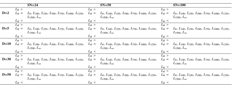
2.2.2. Experiment 2: Vertical Approach with
MaxFEs = 250,000
In this section, there were more fitness evaluations available, and Lk was almost always better than or equal
to other settings. This means that when large enough fitness evaluations were available, Lk was an
appro-priate choice regardless of the population size and di-mension of a problem (for the benchmark suite under investigation). Only for problem f5, which is harder than the other four problems, Lk was in two cases worse
than some other settings. Firstly for SN = 24 and D = 5 and secondly for SN = 24 and D = 10. These differences, however, were never significant. All the differences are shown in Tables 10-14. These findings suggest that set-ting a control parameter ‘limit’ depends on the avail-able maximum number of fitness evaluations.
2.2.3. Experiment 3: Horizontal Approach – 10-6 –
MaxFEs = 1,000,000
During the horizontal approach where we measured the number of function evaluations needed to reach a (sub-)optimal solution, Lk had the better alternatives
in almost all cases. For f1, these better alternatives were
available for the small population size SN = 24 and for the bigger population size SN = 100, whereas for SN = 50, Lk was worse only for D = 5 and better for all other dimension values. For f2, Lk was worse than all the
pop-ulation sizes and dimension values, except for SN = 50 and D = 10, SN = 100 and D = 10, SN = 100 and D = 50, and SN = 100 and D = 50. For f3 and f4, Lk always had a
better alternative and was always worse than at least one other ‘limit’ value, regardless of the population size and dimension of a problem. Lastly, for f5 and small
di-mension D =2 (and any population size values), Lk had
better alternatives, whilst for other dimensions and population sizes all ‘limit’ values performed the same. This happened due to the fact that none of these ‘limit’ values had found the (sub-)optimal solution 10-6 after
1,000,000 fitness evaluations. For D = 2, some ‘lim-it’ values found (sub-)optimal solutions during some runs, and therefore they performed better than Lk.
Whilst there were a lot of differences found between Lk
and other ‘limit’ values, these differences were rarely significant. There were only two problems for which
Lk was significantly worse than some other ‘limit’
val-ues. First was f1 when Lk was significantly worse for
small population size SN =24 for all dimensions. The other was f4 when Lk was significantly worse than all
other ‘limit’ values except L0 for small population size
SN =24 and small dimension D = 2. These differences are shown in Tables 15-19.
2.2.4. Experiment 4: Horizontal Approach 10-12 –
MaxFEs = 1,000,000
In this section, the (sub-)optimal solution was set at 10-12, which was a harder problem than finding (sub-)
optimal solution 10-6. Again, L
k almost always had
a better alternative. For f1 better ‘limit’ values were
found for small population size SN = 24 regardless of dimension D and for the bigger population size SN
=100 where the dimension was greater than D = 2, whilst for SN =50, Lk had better alternatives for small
dimensions D = 2 and D =5 and bigger dimension D = 50. For f2, Lk had better alternatives regardless of the
population size and dimension values. The same went for f3, except when the population size was SN =50 and
dimension D = 5, where Lk was better than the other
fixed ‘limit’ values. For f4, Lk was better than the
oth-er fixed ‘limit’ values when dimension D = 30, whilst for other dimensions (regardless of population size value) there were better alternatives. For f5, all
‘lim-it’ values were the same during performances, which was due to the fact that none of them found the (sub-) optimal solution 10-12 after 1,000,000 fitness
evalua-tions. These differences are shown in Tables 20-24.
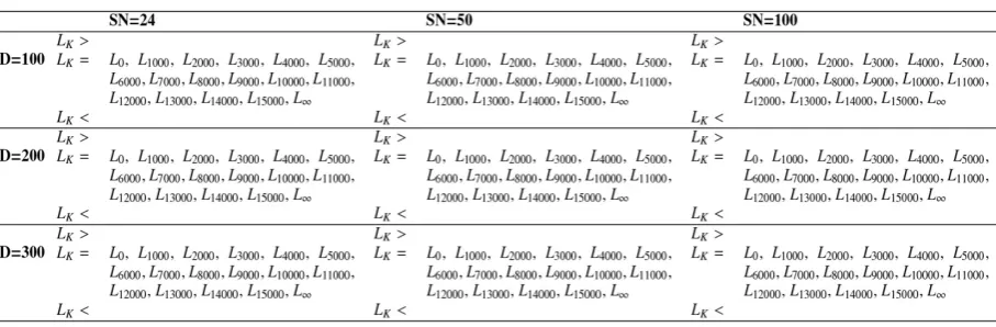
2.2.5. Experiment 5: Large Dimensions
In this section, the horizontal approach with (sub-)op-timal solution set at 10-6 was repeated for larger
dimen-sions, D = {100, 200, 300}, since we have expected that the recommended formulae might perform even worse for large dimensions (such very large optimisation problems are now common for some benchmark suites [32]). Again, fixed ‘limit’ values, L = {0, 1000, 2000, 3000, 4000, 5000, 6000, 7000, 8000, 9000, 10000, 11000, 12000, 13000, 14000, 15000, ∞} were compared to Karaboga’s setting Lk. Found differences are shown
Table 16
f2, horizontal approach, 10-6, NHST
Table 17
f3, horizontal approach, 10-6, NHST Table 15
Table 18
f4, horizontal approach, 10-6, NHST
Table 19
f5, horizontal approach, 10-6, NHST
Table 20
Table 21
f2, horizontal approach, 10-12, NHST
Table 22
f3, horizontal approach, 10-12, NHST
Table 23
Table 24
f5, horizontal approach, 10-12, NHST
Table 25
f1, horizontal approach, 10-6, large dimension, NHST
Table 26
Table 27
f3, horizontal approach, 10-6, large dimension, NHST
Table 28
f4, horizontal approach, 10-6, large dimension, NHST
Table 29
experiment showed that there are other ‘limit’ values that perform better than Lk, for certain problems (f1)
even significantly. In almost all D and SN settings and problems, at least one better performing ‘limit’ value was found (the only exceptions are f1, SN = 50, and D =
200 and f2, SN = 100, and D = 300). For f5, none of the
‘limit’ values reached optimal solution, since all set-tings performed equally. By comparing Tables 25-29 with Tables 15-19, it can be observed that with higher dimensions Lk setting becomes less appropriate.
2.2.6. Discussion
The analysis with NHST supported our concerns about setting a fixed ‘limit’ value regarding the sug-gested formula Lk = ne * D = (SN/2) * D. When a
small-er numbsmall-er of fitness evaluations (e.g., 100,000) wsmall-ere available, Lk was the appropriate choice only for small
dimensions (D = 2, rarely for D = 5 or D = 10) amongst all the five presented problems. When dimension got bigger, more appropriate alternatives could be cho-sen. On the other hand, when sufficiently large enough numbers of fitness evaluations were available (e.g., 250,000), Lk was a significantly better choice than
the presented fixed ‘limit’ values for all the presented problems, dimensions, and values of population size. This does not necessarily mean that a better value than Lk does not exist but it was not defined in our set
of fixed ‘limit’ values.
When it was of interest in finding a (sub-)optimal solution (i.e., 10-6) and a larger number of fitness
eval-uations were available (i.e., 1,000,000), Lk has better
alternatives for the all presented problems, dimen-sions, and values of population size. The only time
Lk seemed to be like an appropriate choice was for
problem f1 (multi-modal, non-separable problem)
when population size equaled 50 and for problem f5
(uni-modal, non-separable problem) for which ABC did not reach the given (sub-)optimal solution over 1,000,000 fitness evaluations regardless of the ‘limit’ value. When the value of this (sub-)optimal solution was even more precise (i.e., 10-12) there were better
alternatives than Lk even for problem f1. In summary,
it was shown that even within this small benchmark suite used in our study setting ‘limit’ is very problem dependent (e.g., see Tables 5-9for results on f1 - f5).
In many cases, better settings existed (even signifi-cantly better) than setting ‘limit’ according to the suggested formula. The results also heavily depended on the number of available fitness evaluations,
indi-cating that ABC convergence with Lk is not amongst
the fastest. The results from the horizontal approach further supported this claim.
2.3. Chess Rating System for Evolutionary Algorithms (CRS4EAs)
The Chess Rating System for Evolutionary Algo-rithms (CRS4EAs) [48] is a novel method for the com-paring and ranking of evolutionary algorithms. In this method, each participating algorithm plays the role of a chess player. The comparison between two players is treated as one game that can have only one out of three outcomes: win, lose, or draw. Two algorithms play a draw whenever the difference in their solutions is smaller than predefined e. Otherwise, the algorithm with the solution closer to the optimum of an optimi-sation problem wins and the other loses. A pairwise comparison between the solutions of all participating algorithms on all optimisation problems over all inde-pendent runs is treated as one tournament. After the tournament has been conducted, the rating R, rating deviation RD, and rating interval RI for each of the players are calculated regarding the formula from the Glicko-2 rating system [16], [17]. Rating is an absolute power of a player that is supported by rating devia-tion. The higher the rating deviation, the less reliable the player’s rating. Rating interval is formed from rat-ing and ratrat-ing deviation. It can be said with 95% prob-ability that a player’s rating R belongs to an interval [R-2RD, R+2RD]. Regarding these rating intervals, the algorithms can then be compared and if their in-tervals do not overlap, the algorithms are considered significantly different. The result of one such tourna-ment is a leaderboard from which all these data can be read and interpreted. When players enter a tour-nament their rating power equals 1500, and their rating deviation equals 350, which is the maximum available rating deviation value. The more games the algorithms play, the smaller become the rating devi-ation values, and the minimum value usually used in CRS4EAs comparisons equals 50.
In this analysis, players were presented as ABC algo-rithms with different ‘limit’ value settings. A tourna-ment was executed for each combination of SN and
differ-ences. Even though, both the Wilcoxon’s test and CRS4EAs compared all runs pairwisely, the results of the Wilcoxon’s test were more relative and the re-sults of CRS4EAs’ more absolute. The Wilcoxon’s test took into consideration only wins and losses against
Lk, which were reflected in the p value. CRS4EAs, on
the other hand, conducted a tournament between 10 players (Lk, L0, L100, L250, L500, L750, L1000, L1250, L1500, L∞)
where runs were pairwisely compared. In regard to these wins, losses, and draws, a rating was calculat-ed and not only were the games against Lk taken into
consideration but games against all opponents. This is the main reason behind the differences between the results of both methods. However, to point out once again: in both approaches, the results were compared as 1×k comparison as CRS4EAs being appropriate for both types of comparisons – 1×k and k×k. There was also a difference in effort put into executing both methods. In CRS4EAs when the ratings of pairwise comparison were obtained, there was no need for fur-ther calculations and testing, whilst when p values are calculated with a statistical test, a post-hoc test, such as the Holm test, is always necessary due to the repetitive comparisons of Lk with other settings.
The experiment was again divided into 4 parts for CRS4EAs analysis. Each part of the experiment took a different approach just as the ones shown in Table 3. For a more straightforward comparison, the reports of rating deviations and rating intervals were omitted in the tables with results, even though they were cal-culated and used in detecting significant differences. The e for determining the draw was set to 10-20 as
re-sults were compared up to 20 decimals places in the Wilcoxon’s test as well. A less precise e would affect the detected differences and there would be great-er diffgreat-erences in NHST and CRS4EAs analyses. The minimum rating deviation value was set at 50 and the maximum rating deviation value at 350. Glicko-2 also calculates some other measurements we omitted during this analysis, as they were unimportant in this analysis. The other CRS4EAs’ parameters used in for-mulae for calculating rating and rating deviation were determined regarding the Glicko-2 rating system. Readers can find more on this topic and definitions of these parameters in [26].
2.3.1. Experiment 1: Vertical Approach with
MaxFEs = 100,000
Tables 30(a) – 30(e)showed the ratings obtained for every setting of SN and D for all 5 minimisation
prob-lems. All the players reached the minimum rating de-viation value of 50 rating points. The best player of each setting (shown in one row) is marked in light grey background colour. For example, from Table 30 (SN = 24, D = 10), it can be observed that the highest rating of 1768 points was obtained using L250 followed by L500
(1693 points), L1000 (1631 points), L750 (1628 points),
L1500 (1603 points), L1250 (1597 points), L∞ (1588 points),
Lk (1394 points), L100 (1116 points), and L0 (982 points).
The difference in rating between the winner L250 (1768
points) and Lk (1394 points) was more than 200 points
(4RD) and hence statistically significant. Overall, these tables show that Lk was not always the more
appropri-ate value for ‘limit’ – especially for f5. However,
observ-ing the ratobserv-ings and when calculatobserv-ing the ratobserv-ing inter-vals as [R-100, R+100] where 100 is 2*RDmin = 2*50, the
differences were rarely significant.
Tables 31-35show more clearly the differences found between Lk and the other 9 fixed ‘limit’ values on all 5
optimisation problems. Whenever the difference was significant, the star symbol (*) has been placed after
Table 30
‘limit’ value, and whenever the Lk had better
alterna-tive(s) the background of table cell has been highlight-ed in light grey colour. Similar to the NHST approach, CRS4EAs also found significant difference only for f1
and f5. In particular, for f1: SN = 24 and D = 10 where Lk
was significantly worse than L250, L500, L750, L1000, L1250,
L1500. For f5: SN = 24 and D = 5 where Lk was
signifi-cantly worse than L250, L500, L750, L1000, L1250, L1500, L∞; SN
= 50 and D = 5 where Lk was significantly worse than
L1000, L1250, L1500, L∞; SN = 24 and D = 10 where Lk was
significantly worse than L750, L∞. However, when
com-paring the detected significant differences between NHST and CRS4EAs (compare Tables 5-9 with Ta-bles 31-35), CRS4EAs appears more conservative than NHST. Whilst the differences were presented for the same settings, in CRS4EAs these differences were hardly ever significant.
For all five problems, Lk had almost always better
al-ternatives (but not significant) when dimension D
was greater (10, 30, or 50).
2.3.2. Experiment 2: Vertical Approach with
MaxFEs = 250,000
Tables 36(a)-36(e)show the ratings obtained for ev-ery setting of SN and D on all 5 minimisation prob-lems. All players reached the minimum rating devia-tion value of 50 rating points. The best player of each setting (shown in one row) is marked in light grey background colour. These tables show that Lk was
almost always the more appropriate value for ‘limit’.
f5 was the only problem for which better alternatives
were found for some SN and D settings. Moreover, Lk
was just as in NHST analysis – the significantly bet-ter choice in most cases.
Table 31
Table 33
f3, vertical approach, MaxFEs = 100,000, CRS4EAs
Table 34
f4, vertical approach, MaxFEs = 100,000, CRS4EAs Table 32
Table 35
f5, vertical approach, MaxFEs = 100,000, CRS4EAs
Table 36
Tables 37-41show more clearly the differences found between Lk and other 9 fixed ‘limit’ values on all 5
op-timisation problems. As mentioned before, the better alternatives were found only for problem f5, when the
dimensions were either 5 or 10 but the ‘limit’ values were not significantly better than Lk. As in NHST
analysis, the CRS4EAs also showed that whenever sufficiently larger numbers of function evaluations were available, Karaboga’s ‘limit’ setting was an ap-propriate choice. In this approach, both methods, NHST and CRS4EAs, appeared equally conservative (compare Tables 10-14 with Tables 37-41).
2.3.3. Experiment 3: Horizontal Approach – 10-6 - MaxFEs = 1,000,000
In the horizontal approach, there were fixed ‘limit’ values that found (sub-)optimal solutions in fewer
fitness evaluations than Lk for all optimisation
prob-lems. Tables 42(a)-42(e)show the ratings for every optimisation problem and every setting of SN and D. All ‘limit’ values reached the minimum rating devia-tion value of 50 rating points and the better rating val-ues are again highlighted with light grey colour. For f1, better alternatives than Lk were available for
the smaller population size SN = 24 and for the greater population size SN = 100, whereas for SN = 50, Lk was
only worse for D = 5 and D = 50 and better for all other dimension values. For f2, Lk was the worst value for all
population sizes and dimensions, except for SN =50 and
D =10, SN = 100 and D = 10, SN = 50 and D = 30, and SN
= 50 and D = 50. For f3, Lk was the better value only for
SN =24 and D =2 and SN =24 and D = 50, but for other settings there were better alternatives. For f4, Lk always
had a better alternative and was always worse than at
Table 37
f1, vertical approach, MaxFEs = 250,000, CRS4EAs
Table 38
Table 39
f3, vertical approach, MaxFEs = 250,000, CRS4EAs
Table 40
f4, vertical approach, MaxFEs = 250,000, CRS4EAs
Table 41
Table 42
Horizontal approach, 10-6
least one other ‘limit’ value, regardless of the population size and dimension of a problem. Lastly, for f5 and small
dimension D =2, Lk had better alternatives, whilst for
other dimensions and population sizes values, all ‘limit’ values performed the same. This happened due to the fact that none of these ‘limit’ values found the (sub-)op-timal solution 10-6 in 1,000,000 available fitness
evalua-tions. For D = 2, some ‘limit’ values found (sub-)optimal solution in some runs, and therefore performed better than Lk. Whilst there were a lot of differences found
be-tween Lk and other ‘limit’ values, these differences were
hardly ever significant. There were only two problems for which Lk was significantly worse than some other
‘limit’ values. The first was f1 where Lk was significantly
worse for small population size SN = 24 and dimension
D = 5. The other problem was f4 where Lk was
signifi-cantly worse than L∞for small population size SN =24
and small dimension D = 2. CRS4EAs again appeared as more conservative than NHST (compare Tables 15-19 with Tables 43-47).
2.3.4. Experiment 4: Horizontal Approach – 10-12 - MaxFEs = 1,000,000
In the horizontal approach with (sub-)optimal solu-tion 10-12, L
k again had better alternatives in almost
all cases. In this approach, Lk was the optimal solution 50% fewer times than when the (sub-)optimal solu-tion equaled 10-6. Tables 48(a)-48(e) show the ratings
obtained for all five optimisation problems.
For f1, Lk always had a better alternative, except when
SN = 50 and D = 10, SN = 50 and D = 30, and SN = 100 and D = 2. For f2, Lk always had a better alternative and
was always worse than at least one other ‘limit’ value, except when SN = 50 and D = 5. For f4, Lk always had a
better alternative and was always worse than at least one other ‘limit’ value, except when SN = 24 and D = 30 and SN = 100 and D = 30. Lastly, for f5, all ‘limit’ values
performed the same. This happened due to the fact that none of these ‘limit’ values found the (sub-)optimal solu-tion 10-12 in 1,000,000 fitness evaluations. Whilst there
were a lot of differences found between Lk and other
‘limit’ values, these differences were rarely significant. There were only two problems for which Lk was
signifi-cantly worse than some other ‘limit’ values. The first was
f1 where Lk was significantly worse for small population
size SN = 24 and dimensions D = {5, 10, 30, 50}. The oth-er was problem f4 where Lk was significantly worse for
small population size SN = 24 and small dimension D = 2. CRS4EAs again appeared as more conservative than NHST (compare Tables 20-24 with Tables 49-53).
2.3.5. Experiment 5: Large Dimensions
In this section, the horizontal approach with (sub-) optimal solution set at 10-6 was repeated for larger
dimensions, D = {100, 200, 300}. Again, fixed ‘limit’ values, L = {0, 1000, 2000, 3000, 4000, 5000, 6000, 7000, 8000, 9000, 10000, 11000, 12000, 13000, 14000, 15000, ∞}, were compared to Karaboga’s setting Lk.
Obtained ratings are shown in Table 54 and found differences are shown in Tables 55-59.As in previous four experiments, this experiment showed that there are other ‘limit’ values that perform better than Lk, for
certain problems (f1) even significantly. In majority
of D and SN settings and problems, at least one better performing ‘limit’ value was found. For f5 none of the
‘limit’ values reached optimal solution, since all set-tings performed equally. By comparing Tables 55-59 with Tables 43-47, it can be observed that with higher dimensions Lk setting becomes less appropriate.
Table 43
f1, horizontal approach, 10-6, CRS4EAs
Table 44
Table 45
f3, horizontal approach, 10-6, CRS4EAs
Table 46
f4, horizontal approach, 10-6, CRS4EAs
Table 47
2.3.6. Discussion
The results between CRS4EAs and NHST were com-parable. When smaller numbers of fitness evaluations were available, Lk was an appropriate choice only for
small dimensions; and when sufficiently large enough numbers of fitness evaluations were available, Lk was
a significantly better choice than the presented fixed ‘limit’ values. When it was of interest to find a (sub-) optimal solution and large numbers of fitness evalua-tions were available, better alternatives than Lkwere
available several times. The main difference between NHST and CRS4EAs comparison was that CRS4EAs was more conservative and detected less significant differences than NHST, however, the conservativi-ty/liberality can be easily controlled through rating deviation RD [48]. Otherwise, the methods showed the same trends when and for which population size and dimension Lk was an unsuitable choice and when
it was a suitable choice. Hence, the main conclusion as presented in Section 2.2.5 is that using NHST was the same as using CRS4EAs. The main differences be-tween both methods showed in the abilities to detect differences amongst fixed ‘limit’ values. Whilst for NHST only the differences between Lk and other fixed
‘limit’ values were calculated and detected, CRS4EAs allowed direct comparisons between fixed ‘limit’ values. In order to find the differences between the fixed ‘limit’ values in NHST, additional tests would be needed, which would be both time consuming and re-quire special care to avoid Type-I-Error.
3. ABC Parameter Tuning
In the previous section, it was shown that ABC does not always perform best when under the setting ‘limit’ Table 48
= ne * D. Hence, the ‘limit’ control parameter should be
tuned or controlled. Therefore, this section displays the results of ABC tuning in contrast to the suggested ‘limit’ setting and to the statistical analysis in Section 2. Tuning is a process of finding those parameter values for which the meta-heuristic algorithm performs the
Table 49
f1, horizontal approach, 10-12, CRS4EAs
Table 50
f2, horizontal approach, 10-12, CRS4EAs
Table 51
f3, horizontal approach, 10-12, CRS4EAs
Table 52
f4, horizontal approach, 10-12, CRS4EAs
Table 53
f5, horizontal approach, 10-12, CRS4EAs
Before the tuning procedure starts, the user has to de-fine the initial set P of all configurations that will be tested, number of initial races r, significance level α under which the statistical tests will be applied, and maximum number of executions. In each iteration, all configurations from P will be executed on one ran-dom problem from the set F over nf independent runs.
After that, if the number of iterations is greater than
r, a Friedman test will be applied to see if there are significant differences amongst all configurations in
P. If the Friedman test shows that there are signifi-cant differences, a post-hoc test, such as Holm test [19] is applied between the best performing config-uration (the one with the smallest Friedman rank) and other configurations. Those configurations that
are significantly worse than the best performing configuration under significance level α are removed from set P. This procedure is repeated until the max-imum number of executions is reached or only one configuration remains in P (Algorithm 2). As already described, one execution is treated as the execution of one configuration on one problem from F over nf
independent runs.
To test the suggested formula for parameter ‘lim-it’ further, we tuned parameters SN and ‘limit’ for different dimensions D on problem f1 with vertical
approach and maximum number of fitness evalua-tions 100,000. The number of independent runs nf
equaled 15,000. A goal of this experiment was to find the parameter values SN and ‘limit’ for which ABC will perform the best on f1 for different dimensions.
Hence, some boundaries and precisions of these two parameters needed to be set. The values parameter
SN could take were {10, 20, 30, ... , 100}, and the values parameter ‘limit’ could take were {0, 50, 100, 150, ... , 1450, 1500, ∞}. These values are different from those used in the experiment in Section 2, as the goal of this experiment is different as well. In this experiment, we wanted to tune the parameters of ABC and in the experiment from Section 2 the goal was to make a pairwise comparison of pre-selected values. In other words, the values of SN and D were fixed in Section 2 and the performances of different ‘limit’ settings compared to Karaboga’s ‘limit’ setting. In this sec-tion, on the other hand, only the allowed values of SN
and ‘limit’ were defined, and the best settings of SN
and ‘limit’ for each fixed value of dimension D were selected with a tuning process. The size of the initial population P equaled 320 (10*32 combinations, 10 for
SN and 32 for ‘limit’). The conclusions of the tuning process are summarised as follows.
_ When the dimensionality of a problem was set to D = 2, 62 configurations remained from the initial set P. The values of parameter SN were from 20 to 100, and the values of parameter ‘limit’ were from 100 to 500. The best performing configurations (those with the lowest Friedman ranks) were {SN = 60, ‘limit’ = 200}, {SN =40, ‘limit’ = 200}, and {SN =80, ‘limit’ = 200}. Following the Karaboga’s formula, the ratio between ‘limit’ and SN when D =2 should be 1:1, meaning that ‘limit’ should have the same value as
SN. None of the configurations found by the tuning process corresponded to this formula.
_ When the dimensionality of a problem was set to
D = 5, 19 configurations remained from the initial set P. The values of parameter SN were from 30 to 50, and the values of parameter ‘limit’ were from 300 to 700. The best performing configurations were {SN =30, ‘limit’ = 300}, {SN = 40, ‘limit’ = 400}, and {SN = 40, ‘limit’ = 550}. Following the Karaboga’s formula, the ratio between ‘limit’ and SN when D = 5 should be 2.5:1, meaning that ‘limit’ should be 2.5-times greater than SN. None of the configurations found by the tuning process corresponded to this formula.
Table 54
Table 55
f1, horizontal approach, 10-6, large dimension, CRS4EAs
Table 56
f2, horizontal approach, 10-6, large dimension, CRS4EAs
Table 57
_ When the dimensionality of a problem was set to D = 10, four configurations remained from the initial set P. The values of parameter SN were 30, and the values of parameter ‘limit’ were from 800 to 1000. Those four configurations were {SN =30, ‘limit’ = 800}, {SN =30, ‘limit’ = 1000}, {SN = 30, ‘limit’ = 950}, and {SN =30, ‘limit’ = 850}. Following the Karaboga’s formula, the ratio between ‘limit’ and SN when D = 10 should be 5:1, meaning that ‘limit’ should be 5-times greater than SN. None of the configurations found by the tuning process corresponded to this formula.
_ When the dimensionality of a problem was set to
D = 30, 70 configurations remained from the initial set P. The values of parameter SN were from 10 to 70, and the values of parameter ‘limit’ were from 700 to ∞. The best performing configurations were {SN = 20, ‘limit’ = 1450}, {SN = 20, ‘limit’ Table 58
f4, horizontal approach, 10-6, large dimension, CRS4EAs
Table 59
f5, horizontal approach, 10-6, large dimension, CRS4EAs
= 1250}, and {SN = 20, ‘limit’ = 1500}. Following the Karaboga’s formula, the ratio between ‘limit’ and SN when D = 30 should be 15:1, meaning that ‘limit’ should be 15-times greater than SN. None of the configurations found by the tuning process corresponded to this formula.
_ When the dimensionality of a problem was set
One would expect that these results can be compared to those in Tables 5 and 31, however as Tables 5 and 31 display the answers to different questions (as already explained above), the results and conclusions of these experiments cannot be compared directly. There are, however, some similarities between the conclusions of both sections. For example, when D = 10 it can be noticed that F-Race found the following best configu-rations: SN = 30 and ‘limit’ = {800, 950, 1000}. Whilst, from Tables 5 and 31 it can be noticed that configura-tions with SN = 24 and ‘limit’ = {750, 1000, 1250} are significantly better statistically than Lk under NHST
and CRS4EAs. Or, when D = 30 it can be noticed that F-Race recommended the following best configura-tions: SN = 20 and ‘limit’ = {1250, 1450, 1500}. Whilst, from Tables 5 and 31 it can be noticed that configura-tions with SN =24 and ‘limit’ = {1000, 1250, 1500} are significantly better statistically than Lk under NHST
and only better, but not statistically significant, un-der CRS4EAs as CRS4EAs is more conservative than NHST in this experiment.
Overall, the results of ABC parameter tuning showed that the best performing configurations did not corre-spond to the Karaboga’s formula for f1. Similar
conclu-sion can be derived from recent study [49] where for ABC parameter tuning F-Race, Revac, and CRS-Tun-ing have been used. From the best performCRS-Tun-ing config-urations found by F-Race, Revac, and CRS-Tuning none conform to the Karaboga formula.
4. Related Work
To date there have been no deep investigations about setting ABC control parameter ‘limit’. The formula ‘limit’ = ne * D was first proposed in the ABC
introduc-tory paper [29] and since then used in many papers (e.g., [6], [21], [24], [27], [28], [31], [54]). The effect of ‘limit’, as investigated by ABC inventors [29], has been studied on the same benchmark suite f1, … , f5
as presented in Section 2 (actually we used the same benchmark suite as in [29]) using the following fac-tors and their values: SN ={20, 40, 100}, D = {2, 5, 50}, and ‘limit’ ={0.1*ne*D, 0.5*ne*D, ne*D, ∞}. However,
full factorial design has not been used since D = 2 was used only for f1, D = 5 for f2, and D = 50 for f3, ... , f5.
Fur-thermore, the only vertical approaches applied in [26] used 20,000 fitness evaluations for f1, f2, and 100,000
fitness evaluations for f3, ... , f5. In our work,
Karabo-ga’s experiment [8] has been extended by performing a full factorial design on this benchmark suite using the following factors and their values: SN = {24, 50, 100}, D = {2, 5, 10, 30, 50}, and ‘limit’ = {0, 100, 250, 500, 750, 1000, 1250, 1500, ∞}, whilst using two differ-ent horizontal and vertical approaches [18]. The other difference between these two studies is that 30 inde-pendent runs were used in [8], whilst 100 in our study in order to enhance its reliability.
The effect of ‘limit’ on ABC was briefly studied in [1] on functions f1 … f5, Ackley and Weierstrass with a
vertical approach (30,000 fitness evaluations, 30 in-dependent runs) using the following factors and their values: SN = {10}, D = {10}, and ‘limit’ = {10, 200, 500, 1000, 3000, 5000}. It was found that ‘limit’ = 200 was more appropriate than other values used in this study. Again, our study can be seen as an extension of [1]. A similar study as in [1] on the effect of ‘limit’ has been recently performed in [30] using a variant of ABC called the quick artificial bee colony (qABC) algorithm. The vertical approach has been applied with 500,000 function evaluations and 30 indepen-dent runs on a benchmark suite containing optimi-sation functions f2, ... , f5. The following factors and
their values have been used: SN= {50}, D = {30}, and ‘limit’ = {10, 50, 187, 375, 750, 1500}. It was found that the ‘limit’ = 750 is the more suitable value, which is equal to the value calculated from the for-mula ‘limit’ = ne * D.
The Enhancing artificial bee colony (EABC) algo-rithm has been proposed in [15] and tested on 48 benchmark functions. The effect of ‘limit’ on EABC was investigated with vertical approach (150,000 function evaluations, 30 independent runs) on seven functions out of 48. The following factors and their values were used: SN = {100}, D = {30}, and ‘limit’ = {50, 100, 200, 400, ∞}. It was reported that ‘limit’ = 200 was the more appropriate than other values used in that study.
‘limit’ is indeed needed. An example of a study where tuning on ‘limit’ was applied is presented in [35]. It is worth mentioning that in all of the above men-tioned experiments, the better settings for ‘limit’ were chosen by visual inspection of the results and without any statistical testing. Our study was quite different to the aforementioned works due to the applications of NHST and CRS4EAs. In this respect, our work was similar to [42], where full factorial design and ANO-VA statistical analysis were used to investigate the sensitivity of reactive tabu search (RTS) to its me-ta-parameters.
5. Conclusions
As the horse racing approach is still omnipresent, researchers have often compared their algorithms, which are well tuned for (a) particular problem(s), with some standard versions of meta-heuristic algo-rithms using recommended control parameter set-tings, which might not be appropriate for some prob-lems used in an experiment. This situation should be avoided. In the recently published guidelines for replication and comparison of experiments in EC [9], we promoted fair comparisons amongst algorithms where all the algorithms used in the comparisons, not only the researchers’ preferred, should be using the best control parameter settings. Hence, performing extensive parameter tuning or control [11] for all al-gorithms involved in an experiment is a prerequisite for a fairer comparison.
This paper has shown that amongst ABC control pa-rameters ‘limit’ is very sensitive, whilst population size (SN) is quite robust (at least for the benchmark suite used in this study). Hence, properly setting con-trol parameter ‘limit’ should be of particular inter-est to every ABC user. Furthermore, it was shown in this study that ABC is not always the best performing when ‘limit’ = (SN/2)*D, although it is a very competi-tive setting. This formula was the best for the vertical approach using 250,000 fitness evaluations for the benchmark suite used in this study. Better settings for ‘limit’ exist, occasionally statistically significant, for the vertical approach using 100,000 fitness evalu-ations, as well as for the both horizontal approaches (reaching (sub-)optimal solution at 10-6 and 10-12) for
benchmark suite used in this study. When 100,000 fitness evaluations were available, Lkwas the
appro-priate choice only for small dimensions (D = 2, rare-ly for D = 5 or D = 10) amongst all the five presented problems. When the dimension becomes bigger, more appropriate alternatives could be chosen. Hence, proper setting of ‘limit’ also depends on the available maximum number of fitness evaluations, indicating that ABC convergence with Lk is not amongst the