USING NEAR-INFRARED PHOTOGRAPHY TO BETTER STUDY SNOW MICROSTRUCTURE AND ITS VARIABILITY OVER TIME AND SPACE
by
Jesse Raymond Dean
A thesis
submitted in partial fulfillment of the requirements for the degree of
Master of Science in Geophysics Boise State University
BOISE STATE UNIVERSITY GRADUATE COLLEGE
DEFENSE COMMITTEE AND FINAL READING APPROVALS
of the thesis submitted by
Jesse Raymond Dean
Thesis Title: Using Near-Infrared Photography to Better Study Snow Microstructure and Its Variability Over Time and Space
Date of Final Oral Examination: 09 November 2016
The following individuals read and discussed the thesis submitted by student Jesse Raymond Dean, and they evaluated his presentation and response to questions during the final oral examination. They found that the student passed the final oral examination. Hans-Peter Marshall, Ph.D. Chair, Supervisory Committee
John Bradford, Ph.D. Member, Supervisory Committee Alejandro N. Flores, Ph.D. Member, Supervisory Committee
iv DEDICATION
v
ACKNOWLEDGMENTS
First and foremost, I would like to thank my advisory committee: Hans-Peter “HP” Marshall, John Bradford, and Alejandro “Lejo” Flores. HP gave me the opportunity to transition from geology to snow science and it was wonderful experience. John and Lejo were critical in educating, enlightening, and guiding me to being able to produce a much more refined thesis. These three have motivated me to strive for an end goal of producing better work and obtaining a more profound understanding of Earth’s systems.
Boise State was my first funding source, as they gave me the opportunity to teach the lab for geology intro courses. Following these labs, they provided me a position as a lab manager. Grants that contributed significant funding include the NASA Harris Grant #NNX11AF27G, Subcontract #A000193404, NASA EPSCoR Grant #NNX10AN30A, the NASA Instrument Incubator Program Grant #NNX11AF27G, and the National Science Foundation (NSF) Hydrologic Sciences Grant #0943710. I greatly appreciate these programs and their continued support of aspiring scientists like myself.
On a personal note, I must thank my Mom and Dad (Claudia and Woody),
vi ABSTRACT
vii
TABLE OF CONTENTS
DEDICATION ... iv
ACKNOWLEDGMENTS ...v
ABSTRACT ... vi
LIST OF FIGURES ... ix
LIST OF ABBREVIATIONS ... xi
INTRODUCTION ...1
BACKGROUND ...5
I. Reflectance Modeling ...5
II. NIR Photography...8
III. Other Optical Methods ...12
METHODS ...15
I. Choosing A Camera...15
II. Camera Construction and Modification ...16
III. Digital Image Files ...19
IV. Image Distortions...21
V. Image Corrections ...22
VI. Snowpit Preparation and Observations ...23
RESULTS ...25
viii
II. A Comparison of Snowpit Data Collection Methods...31
III. A Spatial Comparison of NIR Snowpit Imagery ...36
DISCUSSION ...41
I. NIR Photography for Analyzing Snow Stratigraphy ...41
II. A Comparison of Snowpit Data Collection Methods...44
III. A Spatial Comparison of NIR Snowpit Imagery ...45
IV. Future Work ...47
CONCLUSIONS...49
ix
LIST OF FIGURES
Figure 1. Reflectance of light against wavelength for different snow grain sizes (from Langloiset al., 2010) ... 4 Figure 2. Comparison of calculated and observed albedo versus wavelength for two
unique grain radii (from Wiscombe and Warren, 1980) ... 7 Figure 3. Albedo spectra for four combinations of different contaminant particle
sizes and grain radii (from Warren and Wiscombe, 1980) ... 7 Figure 4. Spectrometry transmission data for the X-Nite850 NIR lens filter
(Llewellyn, 2013) ... 18 Figure 5. A bird’s eye view of Bogus Basin research sites 1 and 2 (Google Earth,
2016) ... 27 Figure 6. NIR image with manual snowpit observations (a,b), ambient and flash
median profile (c), ambient and flash interquartile range (d), and
probability density functions of ambient (e) and flash (f) images ... 29 Figure 7. Ambient NIR image (a), histogram (b), and cumulative distribution
function (c) and flash NIR image (d), histogram (e), and cumulative distribution function (f) ... 30 Figure 8. NIR image with snowpit data (a), Snow Fork wetness (b), AvaTech SP1
NIR emitter/detector pair profile (c), NIR image median (d), and Snow Micro-Penetrometer profiles (e-g) from Site 1 at Bogus Basin on 9 April 2014. Identified correlations have been annotated. ... 34 Figure 9. NIR image and snowpit data (a), NIR image median (b), and Snow
Micro-Penetrometer profiles (c-d) from Site 1 at Bogus Basin on 30 April 2014. SMP correlations are annotated by red boxes. ... 35 Figure 10. Map view of the state of Colorado with the Grand Mesa transect marked
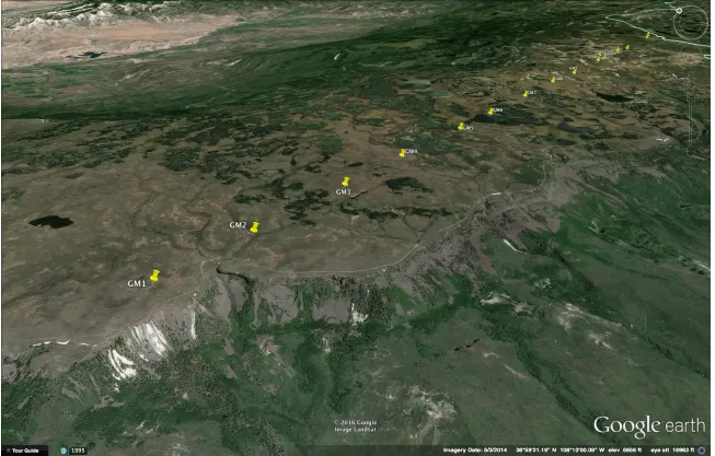
by a yellow pin (Google Earth, 2013) ... 38 Figure 11. Down-line view of the transect from west to east (Google Earth, 2013) . 39 Figure 12. NIR images and snowpit data collected from GM1 (a), GM3 (b), GM6 (c),
x
xi
LIST OF ABBREVIATIONS
SWE Snow-Water Equivalent
SMP Snow Micro-Penetrometer
NIR Near-Infrared
SSA Specific Surface Area
NPP No-Parallax Point
Micro-CT Micro-Computed Tomography ASD Analytical Spectral Devices SWIR Short Wave Infrared
InGaAs Indium-Gallium-Arsenic
DUFISSS Dual Frequency Integrating Sphere for Snow SSA DSLR Digital Single-Lens Reflex
A/D Analog-to-Digital
CMOS Complementary Metal-Oxide Semiconductor
IQ Image Quality
ADU Analog-Digital Unit
RGB Red, Green, and Blue
CFA Color Filter Array
UV Ultra-Violet
MTF Modulation Transfer Function
xii
ICSSG International Classification for Seasonal Snow on the Ground SWAG Snow, Weather, and Avalanche Guidelines
FMCW Frequency-Modulated Continuous-Wave
IQR Interquartile Range
pdf Probability Density Function cdf Cumulative Distribution Function
WISM Wideband Instrument for Snow Measurement
RA1 Reflectance Anomaly 1
1
INTRODUCTION
Seasonal snowmelt dominates over 80% of annual streamflow in the mountainous western United States of America (Serrezeet al., 1999; Barnettet al., 2005). Due to a projected annual warming trend of 0.8-1.7 °C by 2050, maximum stream flow will occur roughly one month sooner in the year (Barnettet al., 2005); combined with limited reservoir storage in the western US, this demands improvements in our understanding of water resources from snowmelt (Barnettet al., 2005). The changing temporal and spatial patterns of snowmelt, caused by changing climate, have large implications on water resources, flood, and avalanche forecasting. With snowfall shifting towards the beginning of the season, certain reservoirs, unable to accommodate the flux, will be forced to
release large volumes of water (Cayanet al., 2001; McCabe and Clark, 2005; Clow, 2009). This will ultimately strain water resources, as reservoirs were designed for a mid- to late-season snowmelt to meet local demand late in the summer. A large enough reservoir release in preparation for a large influx of early season snowmelt will also put areas around downstream rivers and tributaries at risk for flood and subsequent damage.
liquid water to transport through the snowpack. Layer boundaries that exhibit a
significant change in grain size, and sometimes type, can provide an interface for liquid water to transport along, accelerated by gravitational forces (Eirikssonet al., 2013).
On a snowpack scale, stratigraphy complicates Snow-Water Equivalent (SWE) acquisition from spaceborne remote sensing platforms. The current mission concept for measuring SWE from space with active and passive microwave sensors uses changes in radar backscatter and microwave emission. These approaches assume changes are caused by variations in SWE, but these signals are also sensitive to reflections from layer
interfaces and changes in microstructure, independent of changes in SWE. Due to the non-unique nature of reflection profiles produced by variable snow stratigraphy, the accuracy of what is measured can be greatly improved by understanding the microscale properties of the medium.
Current technology used to measure snowpack stratigraphy is time-consuming, technically difficult, and typically provides 1 cm vertical resolution at one location. To observe a snow pit, a researcher must identify layer boundaries, identify grain size and type (at least in the major layers, if not all), test hand hardness, and measure mass at 5 cm increments using a cutter of known volume and a scale (to later calculate density). While it is easily apparent how much time this can take, especially in adverse weather
3
those in this field are prone to subjective bias in their own snow pit observations. As a compounding factor, the nature of these measurements is low resolution. Density is recorded every 5 cm at best, sometimes every 10 cm, and hand hardness profiles can only characterize hardness down to 1 cm (size of your finger).
While collecting these manual snow pit observations is necessary, in order to become more efficient in the field, observers need to supplement this data with time-efficient, simple, high-resolution, and, most importantly, objective tools. The only current tool that satisfies this criteria is the Snow Micro-Penetrometer (SMP), but it is expensive (~$80,000) and equally difficult to transport. Near-infrared (NIR) photography satisfies all the necessary criteria and, unlike the SMP, is extremely cost-effective, and very easy to transport.
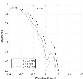
Figure 1 shows how the light reflectance of certain wavelengths changes based on grain size of a particular layer. Between 800 and 1100 nm the reflectance difference between grain sizes is maximized (e.g., Langloiset al., 2010). This is because 800-1100 nm wavelengths are on the order of typical grain sizes in a snowpack. NIR photography harnesses this phenomenon by filtering out wavelengths outside this spectrum, commonly known as near-infrared. Grain sizes vary in both time and space; at a given site, grains will metamorphose over time and change size. This, combined with the grain size-dependent NIR reflectance, provides the framework for a unique analysis of
Without calibration, NIR photography can provide a high-resolution (< 1 mm) map of layer boundaries and measurements of layer roughness (e.g., Tape et. al., 2010). With calibration, NIR photography can be used to estimate Specific Surface Area (SSA; Matzl and Schneebeli, 2006).
Figure 1. Reflectance of light against wavelength for different snow grain sizes
5
BACKGROUND I. Reflectance Modeling
Light interacts with a medium by reflecting off, transmitting through, or being absorbed by that medium. NIR photography records light that has both reflected off and refracted out of the snowpack. Complications arise from many sources, but liquid water, even in small amounts, dramatically affects NIR reflectivity. For this reason, many albedo models operate under the assumption of dry snow.
Stemming from the radiation transmission modeling of gaseous stars by Shuster (1905), Dunkle and Bevans (1956) produce the first formal model of snow by assuming a semi-infinite, homogeneous slab with constant reflection, i.e. isotropic scattering, and absorption coefficients. Although they acknowledge weakness in the assumption of diffuse radiation at normal incidence angles, Dunkle and Bevans (1956) had no information on shallow, directional irradiation. Additionally, impurities increase the absorption coefficient overall, reducing the total reflected light; according to their model, as snow crystals grow, albedo should decrease, which correlates with observations
adjusted absorption rate, k = kdirt + ksnow, accounts for dirt impurities distributed
homogeneously, but can sometimes be neglected (Giddings and LaChapelle, 1961). Bohren and Barkstrom (1974) finally remove the assumption of isotropic scattering, unreasonable in natural snow, and introduce the assumption of spherical ice crystals. They show that for incidence angles not near 90° the reflection coefficient is small and little energy is reflected at an air-ice interface (Bohren and Barkstrom, 1974). This means that the albedo of an ice grain in visible light is dominated by refraction within the grain and not reflection off of its surface, as previously thought (Bohren and Barkstrom, 1974).
In the first of a two-part publication, Wiscombe and Warren (1980) consider dependences on grain size, liquid water content, solar zenith angle, cloud cover, snow thickness, and snow density to model pure snow albedo. Wiscombe and Warren (1980) compare their model results to measured reflectance data of 600-2600 nm wavelengths from O'Brien and Munis (1975) and find respectable agreement between albedo spectra, but much less so in the NIR spectrum (Fig. 2). In the second part of the related
publications, Warren and Wiscombe (1980) find that discrepancies between their pure snow model curves and results from O'Brien and Munis (1975) are easily explained by the presence of atmospheric contaminants. They show that for certain combinations of contaminant particle and grain sizes, the albedo spectra shift dramatically (Warren and Wiscombe, 1980; Fig. 3).
Kokhanovsky and Zege (2004) designed a model of close-packed, fractal ice grains with simple geometrical optics equations instead of Mie scattering. They
7
Figure 2. Comparison of calculated and observed albedo versus wavelength for
two unique grain radii (from Wiscombe and Warren, 1980)
Figure 3. Albedo spectra for four combinations of different contaminant
spectrum where absorption of light is weak relative to other local spectral regions (Kokhanovsky and Zege, 2004).
Until now, this review of albedo modeling has been on dry snow. There have been a few studies of albedo, specifically in NIR light, on wet snow. These studies have
largely used radiometers to measure NIR albedo at the surface (e.g., Chen et al., 2014; Gallet et al., 2014; Hanesiak et al., 2001). Chen et al. (2014) looked at weather station data spanning 18 years to analyze the seasonal evolution of snow albedo at the surface. Gallet et al. (2014) used the DUFISSS instrument (discussed here shortly) with an integrating sphere at 1310 nm to measure SSA of wet snow. Hanesiak et al. (2001) applied surface albedo measurements to airborne video data to extrapolate measurements of various types of snow-covered features; this helped Hanesiak et al. (2001) gather a better understanding of how melt ponds affect albedo over a large area. However, still no study has attempted to measure albedo as it changes with snowpack stratigraphy.
Snow albedo modeling is still in its infancy, but not stagnant in growth. As the need continues to rise for accurate models, such as those that calculate grain size from readily available reflectance data (e.g. satellite imagery), research will progress the community’s understanding of the scattering optics of snow and the underlying physics.
II. NIR Photography
9
preparation of the pit wall, Matzl and Schneebeli (2006) were able to determine true NIR reflectance with a deviation of 2.6%.
Matzl and Schneebeli (2006) used dyed diethyl phthalate to cast 29 individual 70x70x50 mm snow samples of varying grain types from within the image. These samples were analyzed with model-based stereology (i.e. X-Ray Tomography; Baddeley et al., 1986; Matzl, 2006); volume density, resulting in the calculation of snow density, and SSA were both derived from the stereology data (Matzl and Schneebeli, 2006). Matzl and Schneebeli (2006) developed the correlation function, SSA = Aer/t where A = 0.017 ± 0.009 mm-1 and t = 12.222 ± 0.842, by modeling the relationship between stereology-determined SSA values and calculated NIR reflectance. The correlation coefficient, R2, was 90.8% at a significance of p < 0.002 (Matzl and Schneebeli, 2006). The error
increased with increasing SSA; at an SSA of 5 mm-1 error was 4% and at 25 mm-1 it was
15% (Matzl and Schneebeli, 2006). Matzl and Schneebeli (2006) conclude that SSA can be measured in 2-D at a very high resolution with an uncertainty of around 15%. They propose improvements in NIR imaging by recommending the use of cover for diffuse illumination at least 0.5 m behind the pit wall and extending over the sides as well as a flat-field image correction to remove illumination heterogeneities.
Toureet al. (2008) used NIR photography to estimate snow correlation length for microwave emission modeling. Toureet al. (2008) acknowledges that snow hydrologists have traditionally used the largest grain diameter as grain size (Colbecket al., 1990; Armstronget al., 1993), but that leads to an overestimation of effective grain size used in electromagnetic wave scattering models (Maätzler, 2002). Matzl and Schneebeli (2006)
proportional to the relative permittivity correlation length (Debye et al., 1957). Toureet al. (2008) calculated correlation length from NIR reflectance-derived SSA and manually measured snow density using the relationship established by Debye et al. (1957) and
Maätzler (2002).
Tape et al. (2010) studied micro-scale variations in snow stratigraphy with NIR
photography. Further improving the image calibration efforts made by Matzl and
Schneebeli (2006), Tape et al. (2010) corrected for lens distortion (barrel rather than pin-cushion for their equipment) and the NIR bright spot, as most lenses are not designed to
provide consistent transmittance across their image circle for NIR light. To correct for
parallax error, Tape et al. (2010) used a commercially available and affordable panoramic
tripod head to position the camera for rotation about its entrance pupil, or no-parallax
point (NPP), incorrectly referred to as the nodal point in Tape et al. (2010). In an optical
arrangement (i.e. camera lens), there is a front and rear nodal point, but neither are of any
significance to parallax error (Kerr, 2008). PTGui, commercial image-stitching software,
was used to combine laterally adjacent images after lens distortion and NIR illumination
corrections were applied (Tape et al., 2010). A median difference of <2 cm between NIR
image and manually-identified layer boundaries was achieved (Tape et al., 2010).
Recommended applications of this study include estimating thickness and lateral
continuity of structurally weak layers as well as extrapolating manually recorded grain
size and density profiles (Tape et al., 2010).
Assuming a constant shape factor, Langlois et al. (2010) used the simple model
developed by Kokhanovsky and Zege (2004) to calculate NIR reflectance as a function of
11
shown in Figure 1. Langlois et al. (2010) used a large, homogeneous panel under
Lambertian (diffuse) lighting to remove chromatic aberrations and illumination
inconsistencies (NIR bright spot) across the image. To calibrate NIR reflectance, 50%
and nominal 100% (actually 99%) Spectralon NIR reflectance targets were used in the
snow pit image; a five day controlled lab test with 2, 20, 50, 75, and nominal 100%
reflectance targets determined reflectance is consistent and linear with time (Langlois et
al., 2010). Langlois et al. (2010) concluded that NIR photos provide a robust and efficient
method for obtaining a vertical profile of optical grain diameter, assuming a known shape
factor value based upon in-situ grain observations.
Building upon the work primarily by Matzl and Schneebeli (2006), Gergely et al. (2010) aimed to use NIR transmittance photography, where the dominant light source is
diffusely transmitted through rather than reflected off snow layers to determine snow
density. NIR transmittance for a given wavelength only really depends on grain size and
snow density; this is because light absorption increases rapidly moving from visible to
NIR wavelengths and soot-to-ice volume ratios in snow are on the order of 10-9 to 10-6
(Gergely et al., 2010). Density increases cause greater interaction between light and ice
due to close proximity and higher particle density in fine ice grains (Gergely et al., 2010).
Diffuse transmittance can be calculated by Mie theory (van de Hulst, 1958) or by the
DISORT radiative transfer model (Stamnes et al., 1988). Due to user-defined incident
illumination (i.e. diffuse) and computation and output data depths, the DISORT model
was chosen for Gergely et al. (2010). In the case of an infinite snow slab with diffuse
illumination within (i.e. transmittance), the extinction - light that is absorbed and
(Gergely et al., 2010). Micro-computed tomography (micro-CT) was used to estimate
SSA and snow density, as inputs to DISORT (Gergely et al., 2010). While other methods
of measuring SSA exist (e.g. Matzl and Schneebeli, 2006; Painteret al., 2007; Galletet al., 2009), Gergely et al. (2010) also needed density values for their optical transmittance analysis provided by micro-CT. Diffuse transmittance measurements were taken at 830
and 927 nm for 8 snow samples containing melt forms, decomposed, rounded, faceted,
and machine-made snow (Gergely et al., 2010). NIR transmittance results agreed with
DISORT values, calculated using micro-CT-derived SSA and density as inputs, within
the variability of SSA, density, and slab thickness (Gergely et al., 2010).
III. Other Optical Methods
Diffuse NIR reflectance of snow is controlled by SSA, which is equivalent to
optical grain size (Wiscombe and Warren, 1980; Grenfell and Warren, 1999; Zhou et al.,
2003). Gergely et al. (2010) uses three different methods besides NIR photography to
analyze optical properties: InfraSnow (Hug and Trunz, 2006; Frost, 2008), contact
spectroscopy (Painter et al., 2007), and an integrating sphere device (Gallet et al., 2009).
The InfraSnow device was developed to measure grain size near the surface to
study mechanical interactions; it is a hand-held integrating sphere with a 950 nm internal
light source that directly outputs grain size from measured reflectance (Hug and Trunz,
2006; Gergely et al., 2010). While the footprint of the integrating sphere is only 3.5 cm in
diameter, grain size accuracy was 25% for numerous measurements, but errors over 50%
existed due to specular light near the surface and in rough snow (Gergely et al., 2010).
Fortunately, when calibrated to diffuse-reflecting Spectralon targets of known NIR
13
Using an Analytical Spectral Devices (ASD) contact probe and an ASD FieldSpec
FR field spectroradiometer, Painter et al. (2007) provide a source light, measure the
optical response, and invert the 1030 nm absorption component for optical grain radius –
the spherical grain radius that produces the same albedo. The 966 nm (peak wavelength)
light source in a fixed geometry with the probe body helps ease removing the effect of the angular dependence on hemispherical reflectance (Painter et al., 2007). The technique presented by Painter et al. (2007) has a vertical resolution of 2 cm and was shown to produce very accurate, repeatable optical grain radius measurements. However, differences between optical and traditional (manually observed) grain radii, modeled albedo, and associated net shortwave calculations promote a reconsideration of snow metamorphism and grain growth as used by models if modeled grain size is to be used for remote sensing and shortwave radiation purposes.
Gallet et al. (2009) proposed a short wave infrared (SWIR) laser diode oriented
perpendicular to the snow surface and an Indium-Gallium-Arsenic (InGaAs) photodiode
that recorded oriented parallel to the snow surface. Both devices were mounted to a
SphereOptics integrating sphere with an internal SWIR reflectance of 98.5% and an
external SWIR reflectance of 3%; the device was named the Dual Frequency Integrating
Sphere for Snow SSA measurements (DUFISSS; Gallet et al., 2009). Reflectance
calibration curves were calculated with SphereOptics graphite-doped Zenith calibration
targets (Gallet et al., 2009); SSA calibration was done by measuring snow reflectance,
SSA by methane absorption, and reflectance of the sample again to capture any changes
induced by measuring its SSA (Gallet et al., 2009). Two artifacts appeared in their data
artifact was due to their own equipment (Gallet et al., 2009). The sample holder was 13
mm deep initially, which, in low enough density snow, caused the light to reach the
bottom of the sample holder and be absorbed, subsequently hindering an accurate
reflectance measurement (Gallet et al., 2009). Gallet et al. (2009) fixed this issue by using
a 25 mm deep sample holder instead, allowing for lower density snow to be more reliably
measured. The geometry artifact was due to the sample holder sitting below the
integrating sphere; some light scattered will be absorbed by the side walls of the holder
instead of returning to inside the integrating sphere (Gallet et al., 2009). This is inherent
to the design of the instrument and results in the apparent density dependence of their
measurements. The DISORT model was used to calculate hemispherical reflectance and
SSA for 900, 1030, 1310, and 1550 nm wavelengths (Gergely et al., 2010); this showed
that the SSA-reflectance relationship is highly dependent upon wavelength (Gergely et
al., 2010). Gergely et al. (2010) showed that reflectance-derived SSA is twice as accurate
at 1030 nm than 900 nm and three times as accurate than the latter at 1310 nm; 1550 nm
improves upon 1310 nm by providing greater precision for snow with high SSA (Gergely
et al., 2010). Based on their findings, Gallet et al. (2009) recommend using a 1310 nm
source for determining SSA<60 m2/kg and a 1550 nm source for SSA>60 m2/kg. While
not operating at such high resolutions as the methods of Matzl and Schneebeli (2006) or
15
METHODS I. Choosing A Camera
In order to collect NIR photographs, the camera must sensitive to said
wavelengths. Ordinary, off-the-shelf cameras have minimal-to-no NIR sensitivity, as the internal factory filters are intended to accurately reproduce visible light images, but these cameras are readily available and very cost-efficient. For this research, I decided a digital single-lens reflex (DSLR) camera body would be the best to have modified for our use. “Digital” refers to the type of image-recording sensor, “single-lens” refers to the sole lens that attaches to the bayonet (i.e. tab-locking) mount built into the camera body, and “reflex” refers to the articulating mirror inside the camera in front of the sensor. Generally, the more professional-grade DSLRs have higher signal-to-noise ratios than point-and-shoot, consumer-grade cameras, dominantly because the effective pixel area collecting light is larger, allowing more photons to expose a single pixel. More photons collected in a single pixel receptor reduce the necessary gain to be applied and ultimately the amount of noise when sent through the analog-to-digital (A/D) converter. Ultimately, I decided to start with the Canon EOS 60D. The complementary
display) much easier at strange angles in the snow pit. The articulating LCD screen proved itself invaluable when working in adverse weather conditions. Repositioning the screen allowed me to put myself between incoming wind gusts and/or blowing snow and the camera to minimize vibrations or snow sticking to the lens filter, adversely affecting image quality (IQ). IQ, while it is often improperly used in the photographic community to describe subjective observations, should and will refer to objective factors in the data presented here.
II. Camera Construction and Modification
17
emulsion, consistent A/D conversion, lack of inconsistent film developing times and techniques, and lack of other issues related to digitally scanning film negatives.
A digital image sensor functions by capturing photons and accumulating a current at each photodiode while the shutter is open. When the shutter closes, the digital sensor converts that collected current to a voltage, applies a multiplicative gain to bring each voltage within the readable range of an A/D converter, and quantizes each voltage into what may be referred to as an Analog-Digital Unit (ADU). These ADUs measured from each photosite (i.e., pixel) define the RAW camera file, which can be saved as-is to a RAW format or compressed to a JPEG in-camera.
Excluding electrical components used to collect and process a digital image, atop each photodiode in a CMOS sensor is a single-color filter (red, green, or blue; RGB, respectively) overlaid by a micro-lens (FSU website, 2004). These filters are arranged in a color filter array (CFA), which in the case of Canon’s CMOS sensors is made up of Bayer patterns (Bayer, 1976; Canon, 2016). The Bayer array is composed of individual color filters arranged in a two-by-two grid, top left to bottom right, as RGGB (Bayer, 1976). The dyes used to create these RGB filters have transmission spectra that bleed into ultra-violet (UV) and NIR wavelengths (Turchettaet al., 2015). To allow imaging of only visible wavelengths, a glass UV-IR cut filter is mounted on top of the CFA (Llewellyn, 2013). Typical glass compositions like BK7 used by camera companies, such as Canon and Nikon, transmit light from around 360 nm in UV to above the upper sensitivity limit of CMOS sensors at 1100 nm (Llewellyn, 2013).
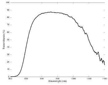
factory-installed UV-IR cut filter and replaced with a custom-cut Schott WG280 UV-VIS-IR filter that transmits from 280 nm to above 1100 nm (Llewellyn, 2013). Installing a UV-VIS-IR filter in place of the factory UV-IR cut filter is necessary to maintain infinity focus of the lens (Llewellyn, 2013). To limit the imaging spectrum to NIR wavelengths only, an X-Nite850 on-lens filter, which screws into the lens’ front filter threads, was purchased from LDP LLC, as well. The X-Nite850 filter has a nominal transmission spectrum of 850-1100 nm; spectrometry data of the X-Nite850 filter, kindly provided by Llewellyn (2013) are in Figure 4.
Figure 4. Spectrometry transmission data for the X-Nite850 NIR lens filter
(Llewellyn, 2013)
19
as an active source. I chose the Canon Speedlite 430EX II for its compact size, affordable price, and lightweight but durable construction. Clarence Spencer of Spencer’s Camera in Alpine, UT modified the flash to fire predominantly NIR light. The source of light inside the 430EX II provides plenty of NIR light and all that was needed was for a 720 nm nominal filter to be attached to the built-in diffusion screen.
III. Digital Image Files
Matzl and Schneebeli (2006), Toureet al. (2008), Langloiset al. (2010), and Tape et al. (2010), among others, do not discuss the file type they are using or why they ultimately chose to use that file type. Hans-Peter Marshall and Martin Schneebeli said that in Tapeet al. (2010) and Matzl and Schneebeli (2006), respectively, JPEG files were used rather than RAW (Schneebeli, 2012; Marshall, 2013). A RAW file is a proprietary container file (e.g., .CR2 for Canon and .NEF for Nikon) or open-source container (e.g., .DNG by Adobe) for the ADU values and descriptive metadata of a given image.
green, or blue-filtered photodiodes are extracted from the RAW file and placed in an m-by-n-by-3 matrix with the third dimension corresponding to the RGB channels,
respectively. Once debayered, the image is intelligently interpolated to fill all empty cells with values (Llewellyn, 2013). The image is now color and tone scale processed; this is a highly complex, non-linear process that most certainly removes all linearity in the RAW data (Llewellyn, 2013). Another step of noise reduction is applied to the image; this time the RGB channels are noise processed to remove aliasing from debayering and
interpolation steps and this process can also be highly non-linear (Llewellyn, 2013). Finally, the processed 16-bit RGB values are rotated into the sRGB color space, reduced to 8-bits (2^8 or 256 values) and compressed into the JPEG format (Llewellyn, 2013).
While the heavily processed and most certainly non-linear JPEG file is an industry standard compressed format for its quality and modest size, in the interest of staying true to the original data, I chose to work with the RAW data. Canon cameras capable of RAW image recording, which includes their 60D DSLR, record the ADU values to a proprietary Canon .CR2 file. The only known processing that is applied the ADU values before they are saved into the RAW container is a gain on the red channel (Llewellyn, 2013). Llewellyn (2013) removes color filter arrays from sensors to make them monochrome and his photos were appearing with a red tint in Adobe Camera Raw; Llewellyn (2013) postulates that the dyes used to cast the R filters do not allow as much power transmission as the G or B dyes, so Canon applies a gain to R channel to
21 container structure. Steve Eddins’ tutorial on the MathWorks blog is a very easy-to-follow, step-by-step guide on how to use the free Adobe DNG Converter to do exactly this and use MATLAB’s Tiff class to import the DNG (Eddins, 2011). Experimental images I collected by maximally overexposing the sensor into a bright light confirmed the ADU scale for a Canon 60D is in fact 14-bits; this means that the scale has 2^14 or 16384 values ranging from 0 to 16383 ADUs.
IV. Image Distortions
Any lens will create some measurable amount of optical distortion. Since lenses are radially symmetric, the distortion can be modeled and removed accordingly. Each lens has a slightly different distortion profile; either the lens induces barrel (outward or “fish-eye”) or pincushion (inward) distortion. The lens I chose for this research came with the Canon EOS 60D in an available kit. It is the Canon EF-S 18-55mm f/3.5-5.6 IS II. Based on a modulation transfer function (MTF) test, which calculates how faithfully the lens reproduces a known source, performed by Photozone, a well-respected German website for lens reviews and information, the lens performs optimally at f/8 (Photozone, 2013).
data. While this effect was not corrected for in this research, it should be noted that it appears negligible and should not affect any quantitative analysis, especially at NIR layer boundaries.
All lenses project an image circle onto the sensor; when the image circle, as determined by the optical arrangement, is significantly larger than the size of the sensor, there is even illumination across the sensor. However, when the image circle is not quite large enough, there is a noticeable fall-off in illumination. This effect is referred to as vignetting. In NIR light, the effect is magnified such that a hot spot of significant brightness appears in the middle of the image circle for most lenses.
The NIR-modified Canon Speedlite 430EX II is an active source of illumination over a range of flash-synchronized shutter speeds. Because the flash provides so much light to the snow pit wall, it cannot be perfectly diffused at the source without using large studio photography softboxes that are unwieldy and expensive. Fortunately, the
cumulative effect between CA, vignetting, the NIR bright spot, and the NIR flash can be recorded by calibration photos with a diffuse-reflecting calibration material covering the pit wall.
V. Image Corrections
23
lighting, both ambient and flash, immediately before the diffuse material was removed and after of the prepared pit face. These diffuse calibration images were median filtered across redundant images and used to normalize the snow layer image, removing any fall-off in lighting. In order to correct for both ambient and flash illumination patterns, calibration images were collected for both cases.
Due to uncontrollable temporal and spatial variations in lighting, all NIR photographs must be reflectance corrected. Two Spectralon calibration targets with known 50% and 99% NIR reflectance were placed in all four corners of each image. Samples within the image of these targets were used to calculate a two-point linear reflectance calibration model between the ADU values and true reflectance.
VI. Snowpit Preparation and Observations
To prepare the snow pit face, I used an avalanche shovel to carefully cut away a nearly flat wall. I then used a plastic crystal card to clear away snow grains until the wall was perfectly flat and smooth down its face.
Manual snow pit observations were made using the current International
Classification for Seasonal Snow on the Ground (ICSSG) 2009 and Snow, Weather, and Avalanche Guidelines (SWAG) 2010 publications (Fierzet al., 2009; Greeneet al., 2010). Standard observations included hand hardness, grain size, grain type, snow density, and temperature profiles.
A snow fork, originally designed by Sihvola and Tiuri (1986), was used to collect a wetness profile with measurements taken every 5 cm down the snow pit wall. The model calculates density and wetness from snow fork-measured dielectric properties (Sihvola and Tiuri, 1986). This model assumes the snow is relatively clean with a pH near 7; if the snow is dirty, its wetness will be overestimated (Sihvola and Tiuri, 1986).
AvaTech, a start-up company out of the Massachusetts Institute of Technology in Boston, MA, has developed the SP1 device that rapidly collects a vertical hardness profile. The AvaTech SP1 device also includes an NIR emitter/detector pair. Comparison between NIR photography and this probe will inform exploration of new,
25
RESULTS
I. A Comparison Between Flash vs. Ambient Lighting
Bogus Basin Ski Area, located 18 km northeast of Boise, ID, was chosen for this study because of its well-instrumented record and accessibility. Site 2 is identified in map view on Figure 5; Site 2 has an east-northeast aspect and typically a deeper, more
stratified snowpack than Site 1.
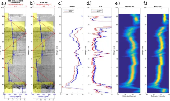
Figure 6 demonstrates the capability of NIR photography to capture complex snow stratigraphy and its spatial variability. Measurements in Figures 6a-b can be
considered below 74 cm, as the flat-field correction material does not cover the pit below this height; this particular limitation was identified at the time and addressed in later data. Series of thin (<1 cm thick) ice lenses are resolved between 41-50 cm and 65-71 cm (Figs. 1a-b). An NIR reflectivity contrast appears at 32 cm above ground; snow
reflectivity appears largely homogeneous between 32 cm and ground (Figs. 6a-b). Low density, relative to the immediately overlying snow, is identified alongside a negative temperature gradient upwards across 0-41 cm; above this from 41-90 cm there is a trend of decreasing density moving up the snowpit (Figs. 6a-b).
The median profile is calculated over 50 rows vertically and all columns
(IQR), calculated for each row and across all columns, detects thin, sloping layers between 41-50 and 65-71 cm, caused by ice lenses (Fig. 6d). However, IQR misses or poorly identifies horizontal, thick layer boundaries recognized by the median. The flash IQR in red sits lower than the ambient in blue, demonstrating it has a lower noise (Fig. 6d). At reflectance contrasts identified by the IQR, the flash profile spikes at or above, in some cases, the ambient demonstrating a higher contrast (Fig. 6d).
27
Figures 7a,d display the NIR reflectivity layers selected from both the ambient and flash images. Histograms of the sampled layers, divided into 50 bins of a width of 1% calibrated intensity value. are displayed by Figures 7b,e. These histograms were normalized, which removes bias attributed to variable sample sizes from within the NIR layers themselves (Figs. 7b,e). For both flash and ambient lighting, histograms suggest the layers did not come from the same sample distribution (Figs. 7b,e). Cumulative distribution functions (cdfs) generated for ambient and flash layers also support the fact that the statistical distributions are unique for each layer. P-values were calculated by first determining all possible combinations of the three layers in each image, ambient and flash, separately. Then, for each possible combination within an image, a two-sample Kolmogorov-Smirnov test (kstest2 function in MATLAB) was performed and in every case returned 0 (Figs. 7c,f). This means the p-values are well below the default threshold of p = 0.05 and it is very unlikely that for each image, ambient and flash, the three layers came from the same distribution (Figs. 7c,f).
Histograms and cdfs of the manually sampled Layer 1 show that the ambient results differ significantly from the flash (Fig. 7b,e). Reflectivity within a fairly
29
Figure 6. NIR image with manual snowpit observations (a,b), ambient and flash median profile (c), ambient and flash
30
Figure 7. Ambient NIR image (a), histogram (b), and cumulative distribution function (c) and flash NIR image (d),
31
flash NIR image over the ambient. Ambient Layer 1 data differs from the flash most likely because of non-homogeneous lighting conditions during ambient image collection. The pit was not covered, as can be seen in the tops of Figures 7a,d, which allowed non-diffuse light to cause the upper layers of the snow pit to appear brighter than the lower layers in NIR light.
II. A Comparison of Snowpit Data Collection Methods
To obtain a dataset that provides unique and valuable insight into the similarities and differences and strengths and weaknesses of NIR photography against other, more established snowpit methods, I studied the snowpack of our Site 1 at Bogus Basin Ski Area (Fig. 5). Site 1 presents a slope with variable land cover that has been
well-instrumented and regularly studied in winters past. For this study, NIR photography was collected alongside manual observations, Snow Fork wetness, AvaTech SP1 profiles, and Snow MicroPenetrometer (SMP) data. Data collected on 9 and 30 April 2014 will be used for these comparisons; spring melt had begun so the snowpack was wet.
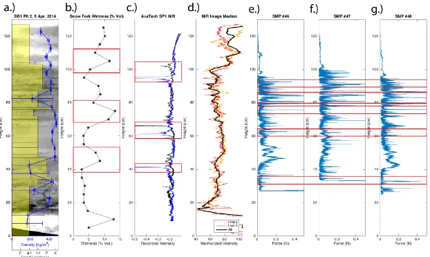
On 9 April 2014, NIR reflectivity anomalies at 34, 44, 75, 88, and 102 cm correlate with manually observed layer boundaries at 35, 46, 77, 88, and 103 cm (Fig. 8a). On 30 April 2014, NIR reflectivity anomalies at 21, 33, 36, 70, 72, and 76 cm
The snowpack was very wet on 9 April 2014. Moving from top to bottom in the snowpit there exists a trend where wetness increases above, then sharply decreases below, a low NIR reflectivity layer identified as an ice lens (Fig. 8b). This phenomenon occurs across layers at 44, 75, and 102 cm (Fig. 8b). Because of the strong correlation between immediate increases in wetness and observed hard layers in the snowpack, these data show the stratigraphic location where liquid water is pooling in the snowpack. No Snow Fork data was collected on 30 April.
The AvaTech SP1 NIR emitter/detector pair identified extremely low reflectivity anomalies in one profile (blue) at 41, 66, and 95 cm and in a second profile (black) at 61 and 102 cm (Fig 8c). Considering the extremely high spatial variability of snow
stratigraphy, low reflectivity anomalies between the two profiles at 61 (blue) and 66 (black) cm as well as 95 (blue) and 102 (black) cm are likely produced by the same reflectance contrast in the snowpack. These low reflectivity anomalies correlate to
observed layer boundaries and the sharp increases in Snow Fork wetness (Fig. 8a-c). Due to these correlations, the AvaTech SP1 NIR emitter/detector pair is also detecting
concentrations of liquid water because water strongly absorbs NIR light. Putting this NIR emitter/detector pair in the context of NIR photography, it is like extracting one column of NIR reflectance measurements from an NIR image; an NIR photo shows how variable this reflectivity is across the pit wall. No AvaTech SP1 data was collected on 30 April 2014. Median processing of the NIR image supports both the aforementioned
33
On 9 April, the SMP was used to measure undisturbed snow behind the face of the exposed snowpit (Fig. 8e-g). Correlated hardness anomalies vary up to 8 cm within 1 m2 of the snowpack (Fig. 8e-g). High hardness anomalies in the SMP data at 34, 62, 76, 81, 84, and 90 cm that correlate to low NIR reflectivity anomalies at 35, 62, 77, 81, 84, and 90 cm (Fig. 8e-g). These anomalies are in-part identified as ice layers by manual observation at 35, 77, and 87 cm and are also locations where liquid water was
concentrated. On 30 April, the SMP probed additional profiles adjacent to the exposed snowpit in undisturbed snow (Fig. 9c-d). Between the two profiles there is good
34
Figure 8. NIR image with snowpit data (a), Snow Fork wetness (b), AvaTech SP1 NIR emitter/detector pair profile (c),
35
Figure 9. NIR image and snowpit data (a), NIR image median (b), and Snow Micro-Penetrometer profiles (c-d) from Site
III. A Spatial Comparison of NIR Snowpit Imagery
From 20-25 February, 2015, the NASA Wideband Instrument for Snow
Measurement (WISM) project flew airborne LiDAR, radar, and radiometer instruments on Grand Mesa, supported by an extensive ground-truthing campaign, along a 20 km transect. The transect itself can be seen in map view in relation to the state of Colorado in Figure 10. The transect ran roughly west to east and stretched across both unprotected and protected meadows and frozen lakes, and its west end, at the edge of the mesa, was just north of a sheer vertical cliff face. A down-line view of the transect is shown in Figure 11.
This site was identified to have an increase in SWE from west to east due to either changes in land cover or the interaction between wind and topography, not due to
37
well (Fig. 12), but is a clear, thin layer with different microstructure than the adjacent layers. These kinds of layers are hard to identify in the field, and underscores the benefit of combining NIR photography with traditional snow observations. Three other local RAs are identified and matched between GM8 and GM10 with solid cyan lines (Fig. 12); these three local RAs only partially agree with manual observations (Fig. 12). An ice-facet layer boundary (LB1), unassociated with RA1, is identified and is traced in purple across all snowpits in Figure 12 but with lower confidence east of GM6 due to a change in precipitation and overall weather pattern made obvious by the increased snow
deposition. It is important to note that while descriptions of these qualitative correlations between NIR and observed layer boundaries may seem easy to have confidence in, all correlations made are suggested; there are no absolutely definitive correlations between snowpits in these data.
38
39
40
Figure 12. NIR images and snowpit data collected from GM1 (a), GM3 (b), GM6 (c), GM8 (d), and GM10 (e) between
20-21 February 2015 in Grand Mesa, Colorado. Manually observed snowpit boundaries and NIR reflectance layers connected by solid and dashed lines as noted in the legend. Manual snowpit data shown in (e) has been shifted 8 cm vertically to better align
41
DISCUSSION
I. NIR Photography for Analyzing Snow Stratigraphy
The horizontal resolution provided by NIR photography demonstrates how spatially variable snow can be. Stratigraphic layers are not necessarily parallel to the snow-ground (bottom) or snow-air (top) pit surfaces. In Figure 6, low density and a negative temperature gradient below 41 cm suggest basal faceting (depth hoar), which is likely the cause of lower reflectivity. Also in Figure 6, the upward trend of decreasing density above 41 cm is likely caused by settling and compaction under the cumulative weight of overlying snow.
exits the snowpack at a complementary angle; light returned to the camera sensor from the bottom of the snowpit will be of lower intensity than that from the top. This fairly obvious effect best explains why in Figure 6c the flash image median is greater in the upper half and lesser in the lower half than the ambient one. So as far as being able to compare relative differences between NIR layers is concerned, ambient light appears to be the better approach. This is because of its more consistent illumination down the pit wall and the ease of keeping these lighting conditions consistent between snowpits.
Looking at the IQR of NIR images, more dramatic contrasts become readily apparent. Ice lenses, especially those between 41-50 cm, which are less than 1 cm thick or the width of an observer’s finger, stand tall above from the noise floor and demonstrate the very useful nature of this type of statistical processing (Fig. 6d). In Figure 6d, the ambient IQR noise floor is consistently greater than the flash; the only time it is not greater is when the two are equal at IQR spikes. Since the two are equal when they spike and the flash IQR shows a lower noise floor, this demonstrates that the flash provides an increase in contrast among recorded intensities over the ambient-lit image. The use of an NIR flash is certainly promising and appears to be superior to ambient light, but first a way to fully diffuse the light source to uniformly expose the pit wall must be developed. Once a uniform field of light can be generated, many of the current complications and shortcomings of flash NIR will be resolved soon-after.
A non-parametric pdf calculated for the amplitudes of each of the ambient and flash NIR images combines benefits of median and IQR processing and provides a simple and intuitive look at the distribution of recorded intensities down the snowpit. This
43
visualization. Both the subtler grain size and shape change at 32 cm and prominent ice lenses between 41-50 and 65-71 cm are highlighted in the pdf (Fig. 6e-f). The ambient pdf has a more wide and flat shape than the flash and the flash spikes higher in the z -direction (height in z is proportional to color warmth) and deviates less about its median in x than the ambient (Fig. 6e-f). To proceed with an attempt to automatically detect layer boundaries in an NIR image, using the pdf of the NIR image would be advantageous, as it identifies the widest range of reflectivity contrasts in a single analytical tool.
Increased contrast of flash over ambient demonstrated by IQR and pdf plots (Figs. 6d-f) is facilitated by the shutter speed as these ambient and flash NIR images capture photons over the same, short length of time. Since the sample times are equal between these images, the resulting scales of RAW intensity are also comparable; RAW refers to the most original form of data recorded by the camera ideally with zero compression. No additional sample time for either image means the maximum number of photons captured by any single pixel site remains the same; the minimum photon count is obviously always zero. RAW intensity is therefore proportional to the total number of photons collected at a given pixel site and can be compared between different images of equal sample time. Because these images have been calibrated both to a homogeneous reflectance surface and targets of known NIR reflectance, the equal shutter speed (sample time) point is rendered moot (Fig. 6).
minimize changes in lighting conditions, one can compare images of equal shutter speed without additional calibration for certain objective purposes (i.e. analyzing relative reflectivity changes between pits). This allows for a very compact field kit (an NIR-modified camera alone) to produce rapidly-collected, high-resolution, comparable, and objective data from highly variable snowpacks with only an elementary knowledge of photography principles and be done at a considerably lower cost than alternative methods.
II. A Comparison of Snowpit Data Collection Methods
45
In the case of 30 April data, median values of the NIR image once again provides the ability to delineate layer boundaries (Fig. 9b). Spikes in both SMP profiles correlate well with jumps in the NIR median profile at 32, 35, 43, 49, and 73 cm in SMP #98 and 32, 35, 40, 48, 65, 77, and 83 cm in SMP #99 (Fig. 9). Consistency in correlation between NIR reflectivity and SMP strength contrasts demonstrates the usefulness of combining and comparing the results from multiple methods to study snow. Insights gathered from a single geophysical method are supported and potentially further refined by the comparison with other techniques, often observing entirely different phenomena or electromagnetic/material properties.
III. A Spatial Comparison of NIR Snowpit Imagery
In all snowpits measured for this study at Grand Mesa, CO, there was an observed dust layer. The appearance of snow stratigraphy in visible light is dominantly affected by impurities, but not by grain size (Painter et al., 2013); in NIR light, its appearance is dominantly affected by changes in grain size, not by the presence of impurities (Langlois et al., 2010). This dust layer, noted by the snowpit observers, does not appear in any of the NIR photographs. Observation of the dust layer in visible light by the naked eye and lack of evidence of its presence in the snow stratigraphy in NIR photographs supports the accepted theory of the interaction between different types of light, impurities, and grain size in snow as described by Painter et al. (2013) and Langlois et al. (2010).
frozen, so most of the snow melts away immediately. Once the lake has frozen and snow begins to accumulate, the lake water is warmer than the frozen lake surface creating a negative upward temperature gradient to the cold air above the top of the snowpack. Snow melt and metamorphosis happen at a much faster rate due to this extreme
temperature gradient. Thus, while LB1 appears very similar in GM6 in composition and hardness to the naked-eye, similar in NIR reflectivity, and is likely the same layer, due to the vastly different circumstances under which it formed it must be an implied
correlation. Unfortunately, not every NIR snowpit image reveals a layer that can be identified as the manually observed LB1 (Fig. 12).
RA1 is an NIR reflectance anomaly correlated across the transect by a solid green line in Figure 12. It is important to note that LB1 identified under manual observation is not able to be reliably correlated to an NIR reflectivity layer across the transect (Fig. 12). Also, from just manual snowpit observation it is equally challenging to identify RA1 as any one layer in manual observation data. This supports our accepted theoretical
understanding of how snow grain size and shape are the two most prominent controls on NIR reflectivity. An inadequate change in grain size and shape will not produce an NIR reflectance contrast in the snowpit image, just as how human error and the difference in interaction of snow and visible light versus NIR affect the ability of a layer to be
47
IV. Future Work
Stemming directly from qualitatively correlating layers on the Grand Mesa, CO, data, the very next work should be an attempt to quantitatively correlate NIR layers between snow pits. This can be done one of two ways. Either the calibrated reflectance values can be correlated within a given tolerance between NIR snowpit images or these reflectance values can be converted to SSA and then to grain size using the method devised by Matzl and Schneebeli (2006) and compared to the manual grain size observations.
Snow grain anisotropy exists in certain grain types (e.g. basal facets a.k.a. depth hoar) that build connected vertical chains of crystals by the mass movement process of sublimation and deposition. The NIR reflectance contrast between air and ice is sufficient to allow a noticeable change in recorded intensity in an NIR image. Thus, NIR
photography allows the observer to record an image that identifies these unidirectional, connected crystal chains that stand in contrast against the empty matrix they occupy. Observing this phenomenon in NIR light with simultaneous manual observation and measurement using microwave radar techniques could provide valuable insight into better understanding how reflections occur along layer boundaries and how energy is scattered by common grain types that make up most layers.
with lower individual power output providing a more evenly distributed blanket of light over the imaged area that could be better diffused by a semi-transparent scattering
medium. After this equipment is constructed, the focus should then turn to calibrating the power output and spectrum of the LED light grid and the images themselves to attempt to quantify the amount of liquid water.
Following an exploration into using very carefully calibrated active-source NIR photography to quantify liquid water content, a minimally-destructive probe, much like the AvaTech SP1, to measure and quantify stratigraphic properties should be considered. Useful values this probe could attempt to measure and/or calculate include liquid water content, SWE, and SSA. Other valuable sensors to consider including on such a device would be multiple resolution NIR emitter/detector pairs and an infrared temperature sensor.
49
CONCLUSIONS
In a general sense, data from NIR photography and manual snowpit observations are best collected and analyzed together. Combining data from the NIR and visible spectrums allows us to exploit the widest range and difference in electromagnetic properties of snow to build a more complete understanding of a rapidly evolving
snowpack. NIR reflectance, primarily controlled by snow grain size and shape, should be used to compliment hardness, density, and temperature measurements and reinforce or quality-check manual grain size and type observations.
NIR photography lets us revisit a snowpack and take a closer look at exactly how, predominantly, grain size and shape change. NIR imagery helps us identify certain layers often missed by manual observers; this is especially true for thin layers, particularly those less than 1 cm wide or the width of an observer’s finger. The resolution provided by NIR photography is unparalleled for the price. Cameras readily available with at least 15 million pixels have the ability to zoom in to below the millimeter scale to study changes vertically and horizontally. This is crucial to gathering a meaningful understanding of the properties and processes at work. This sub-millimeter resolution for less than $500 is in a ballpark all its own; if you want to measure stratigraphy at a comparable resolution, you need an SMP that costs approximately $50,000.
processing and demonstrate the higher contrast and lower noise floor associated with using an active light source rather than a passive one.
NIR photography is sensitive to two phases of water: solid and liquid. The Snow Fork measures what can be considered bulk wetness, or an integrated measurement from about a 5-10 cm diameter sphere around the electrical prongs that are inserted into the snowpack. NIR imagery shows the distribution of this liquid water and where it is
pooling atop ice lenses when analyzed alongside wetness data. Using a technique such as the NIR emitter/detector pair in the AvaTech SP1 probe can also identify the stratigraphic distribution of liquid water because liquid water strongly absorbs NIR light causing very low reflectance anomalies. This reinforces the importance of corroborating data from multiple methods.
It is always important to consider evidence from various methods in order to gain the best picture and therefore understanding of the snowpack in question. NIR
photography is an affordable method to rapidly collect and process images that record and allow for the correlation of snow layer boundaries at variable heights above ground across space and time. Introducing a flash into NIR photography research has improved and expanded existing NIR techniques and applications. Currently, the NIR flash is not properly diffused and needs to be to provide uniform illumination of the pit wall. Until the flash can be uniformly distributed down the pit wall, ambient-lit NIR photography is the superior technique to analyze layer stratigraphy and from which to obtain quantitative reflectance measurements.
51
REFERENCES
Armstrong, R. L., A. Chang, A. Rango and E. Josberger (1993). "Snow depths and grain-size relationships with relevance to passive microwave studies." Annals of Glaciology 17: 171-176.
Baddeley, A. J., H. J. G. Gundersen and L. M. Cruz-Orive (1986). "Estimation of surface area from vertical sections." Journal of Microscopy 142(3): 259-276.
Barnett, T. P., J. C. Adam and D. P. Lettenmaier (2005). "Potential impacts of a warming climate on water availability in snow-dominated regions." Nature 438(7066): 303-309. Bayer, B. E. (1976). Color imaging array. U. S. P. a. T. Office. United States of America,
Eastman Kodak Company.
Bohren, C. F. and B. R. Barkstrom (1974). "Theory of the optical properties of snow." Journal of Geophysical Research 79(30): 4527-4535.
Canon (2016) "EOS HD (DSLR) White Paper." Canon EOS and Adobe Premiere Workflow Cayan, D. R., M. D. Dettinger, S. A. Kammerdiener, J. M. Caprio and D. H. Peterson (2001).
"Changes in the Onset of Spring in the Western United States." Bulletin of the American Meteorological Society 82(3): 399-415.
Chen, A., W. Li, W. Li, and X. Liu (2014). “An observational study of snow aging and the seasonal variation of snow albedo by using data from Col de Porte, France.” Chinese Science Bulletin 59(34): 4881-4889.
Clow, D. W. (2009). "Changes in the Timing of Snowmelt and Streamflow in Colorado: A Response to Recent Warming." Journal of Climate 23(9): 2293-2306.
Colbeck, S., E. Akitaya, R. Armstrong, H. Gubler, J. Lafeuille, K. Lied, D. McClung and E. Morris (1990). The International Classification for Seasonal Snow on the Ground, University of Colorado, Boulder, CO, USA.
53
Dunkle, R. V. and J. T. Bevans (1956). "An approximate analysis of the solar reflectance and transmittance of a snow cover." Journal of Meteorology 13(2): 212-216.
Eddins, S. (2011) "Tips for reading a camera raw file into MATLAB."
Einstein, A. (1905). "Investigations on the theory of the Brownian Movement." Annalen der Physik 17 549-560
Eiriksson, D., M. Whitson, C. H. Luce, H. P. Marshall, J. Bradford, S. G. Benner, T. Black, H. Hetrick and J. P. McNamara (2013). "An evaluation of the hydrologic relevance of lateral flow in snow at hillslope and catchment scales." Hydrological Processes 27(5): 640-654.
Fierz, C., R. L. Armstrong, Y. Durrand, P. Etchevers, E. Greene, D. M. McClung, K.
Nishimura, P. Satayawali and S. A. Sokratov (2009). The International Classification for Seasonal Snow on the Ground, International Association for Cryospheric
Geosciences.
Frost, D. (2008). Calibration, testing and design of a hand-held instrument for outdoor measurements of the grain size and temperature of snow, Autonomous System Lab (ASL), Swiss Federal Institute of Technology Zürich.
Gallet, J. C., F. Domine, C. S. Zender and G. Picard (2009). "Measurement of the specific surface area of snow using infrared reflectance in an integrating sphere at 1310 and 1550 nm." The Cryosphere 3(2): 167-182.
Gallet, J. C., F. Domine, and M. Dumont (2014). “Measuring the specific surface area of wet snow using 1310 nm reflectance.” The Cryosphere 8: 1139-1148.
Gergely, M., M. Schneebeli and K. Roth (2010). "First experiments to determine snow density from diffuse near-infrared transmittance." Cold Regions Science and Technology 64(2): 81-86.
Giddings, J. C. and E. LaChapelle (1961). "Diffusion theory applied to radiant energy distribution and albedo of snow." Journal of Geophysical Research 66(1): 181-189. Google Earth (2013). 39°52'14.79" N, 107°47'58.47" W, Elevation 8200 ft. Google Earth 7. Google Earth (2016). 43°45'54.86" N, 116° 5'12.21" W, Elevation 7140 ft. Google Earth 7. Greene, E., K. Birkeland, K. Elder, C. Landry, B. Lazar, I. McCammon, M. Moore, D. Sharaf,
Observational Guidelines for Avalanche Programs in the United States, American Avalanche Association.
Grenfell, T. C. and S. G. Warren (1999). "Representation of a nonspherical ice particle by a collection of independent spheres for scattering and absorption of radiation." Journal of Geophysical Research: Atmospheres 104(D24): 31697-31709.
Hanesiak, J. M., D. G. Barber, R. A. De Abreu, and J. J. Yackel (2001). “Local and regional albedo observations of arctic first-year sea ice during melt ponding.” Journal of Geophysical Research 106(C1): 1005-1016.
Hug, M. and S. Trunz (2006). InfraSnow.
Johnson, J. B. and M. Schneebeli (1999). "Characterizing the microstructural and
micromechanical properties of snow." Cold Regions Science and Technology 30(1–3): 91-100.
Kerr, D. A. (2008) "The Proper Pivot Point for Panoramic Photography."
Kokhanovsky, A. A. and E. P. Zege (2004). "Scattering optics of snow." Applied Optics 43(7): 1589-1602.
Langlois, A., A. Royer, B. Montpetit, G. Picard, L. Brucker, L. Arnaud, P. Harvey-Collard, M. Fily and K. Goïta (2010). "On the relationship between snow grain morphology and in-situ near infrared calibrated reflectance photographs." Cold Regions Science and Technology 61(1): 34-42.
Llewellyn, D. (2013). Personal communication. J. Dean.
Maätzler, C. (2002). "Relation between grain-size and correlation length of snow." Journal of Glaciology 48(162): 461-466.
Marshall, H. P. (2013). Personal communication. J. Dean.
Matzl, M. (2006). Quantifying the stratigraphy of snow profiles. Doctor of Science, Swiss Federal Institute of Technology Zürich.
Matzl, M. and M. Schneebeli (2006). "Measuring specific surface area of snow by near-infrared photography." Journal of Glaciology 52(179): 558-564.
McCabe, G. J. and M. P. Clark (2005). "Trends and Variability in Snowmelt Runoff in the Western United States." Journal of Hydrometeorology 6(4): 476-482.
55
Painter, T. H., N. P. Molotch, M. Cassidy, M. Flanner and K. Steffen (2007). "Contact spectroscopy for determination of stratigraphy of snow optical grain size." Journal of Glaciology 53(180): 121-127.
Painter, T. H., F. C. Seidel, A. C. Bryant, S. McKenzie Skiles, and K. Rittger (2013). “Imaging spectroscopy of albedo and radiative forcing by light-absorbing impurities in mountain snow.” Journal of Geophysical Research: Atmospheres 118: 9511–9523.
Photozone. (2013). "Canon EF-S 18-55mm f/3.5-5.6 STM IS - Review/Test Report." Retrieved 2 June 2016, from http://www.photozone.de/Reviews/180-canon-ef-s-18-55mm-f35-56-ii-test-report--review.
Schneebeli, M. (2012). Personal communication. J. Dean.
Schneebeli, M. and J. B. Johnson (1998). "A constant-speed penetrometer for high-resolution snow stratigraphy." Annals of Glaciology 26: 107-111.
Serreze, M. C., M. P. Clark, R. L. Armstrong, D. A. McGinnis and R. S. Pulwarty (1999). "Characteristics of the western United States snowpack from snowpack telemetry (SNOTEL) data." Water Resources Research 35(7): 2145-2160.
Shuster, A. (1905). "Radiation through a foggy atmosphere." The Astrophysical Journal 21(1): 1-22.
Sihvola, A. and M. Tiuri (1986). "Snow Fork for Field Determination of the Density and Wetness Profiles of a Snow Pack." IEEE Transactions on Geoscience and Remote Sensing GE-24(5): 717-721.
Stamnes, K., S. C. Tsay, W. Wiscombe and K. Jayaweera (1988). "Numerically stable algorithm for discrete-ordinate-method radiative transfer in multiple scattering and emitting layered media." Applied Optics 27(12): 2502-2509.
Tape, K. D., N. Rutter, H.-P. Marshall, R. Essery and M. Sturm (2010). "Recording microscale variations in snowpack layering using near-infrared photography." Journal of
Glaciology 56(195): 75-80.
Turchetta, R., K. R. Spring and M. W. Davidson. (2015). "Molecular Expressions: Optical Microscopy Primer: Digital Imaging in Optical Microscopy." Retrieved 2 June 2016, from http://micro.magnet.fsu.edu/primer/digitalimaging/cmosimagesensors.html. van de Hulst, H. C. (1958). "Light scattering by small particles." Quarterly Journal of the Royal
Meteorological Society 84(360): 198-199.
Warren, S. G. and W. J. Wiscombe (1980). "A Model for the Spectral Albedo of Snow. II: Snow Containing Atmospheric Aerosols." Journal of the Atmospheric Sciences 37(12): 2734-2745.
Wiscombe, W. J. and S. G. Warren (1980). "A Model for the Spectral Albedo of Snow. I: Pure Snow." Journal of the Atmospheric Sciences 37(12): 2712-2733.