Secrecy Constrained Distributed Inference in Wireless Sensor Networks

DEFENSE COMMITTEE AND FINAL READING APPROVALS

of the dissertation submitted by

Jun Guo

Dissertation Title: Secrecy Constrained Distributed Inference In Wireless Sensor Net-works

Date of Final Oral Examination: 7th April 2017

The following individuals read and discussed the dissertation submitted by student Jun Guo, and they evaluated his presentation and response to questions during the final oral examination. They found that the student passed the final oral examination.

Hao Chen, Ph.D. Chair of the Supervisory Committee

John Chiasson, Ph.D. Member, Supervisory Committee

Leming Qu, Ph.D. Member, Supervisory Committee

Qi Cheng, Ph.D. External Examiner

In his book, The Ph.D. Grind, Philip Guo wrote, “there would be no Ph.D. without ten thousand hours of unglamorous, hard-nosed grinding”. I have the same feeling about my pursuit of Ph.D., which is closing to an end. However, I do not think hard work alone is enough for me to come so far without the guidance, encouragement and support from my advisor, professors, family and friends. So, I would like to express my gratitude to all of them on this page.

I am deeply indebted to my advisor, Dr. Hao Chen, for his belief in me from the very beginning and patient guidance on my research during the course of my Ph.D. study. I have learned a great deal on statistical inference from Dr. Chen, but one thing I am most impressed is his mathematical intuition. “Our intuition is based on accumulated and compiled experiences, not on magic”, mentioned in the book,

The power of intuition, which means it is not something that one can pick up in a short amount of time; however it motivates me to keep accumulating, learning and thinking for the rest of my life. Besides, his sharpness and humor make me feel that he is more like a mentor and a caring friend, who also gave me freedom and support to collaborate with other professors and researchers on signal processing and machine learning projects.

I am grateful to Dr. John Chiasson, Dr. Leming Qu, and Dr. Qi Cheng for serving in my committee. Dr. Chiasson’s machine learning course motivated me to dive into the field of deep learning. We often discuss things beyond engineering topics and his humor definitely made my Ph.D. life more pleasant.

I am really fortunate to have friends, Kehan Zhu and Mucun Tian during the course of my doctoral study. Throughout these years, we encourage and help out each other on research and daily lives.

This thesis is dedicated to my mother for the unconditional love, support and belief in me. To my sister, Jin, who always cares me deeply in her heart and taught me to be a resilient person. To my wife, Yuwen, who helps me find my inner peace and gives strength to keep exploring the road less traveled. To my child, who always reminds me to have a beginner’s mind.

Last but not the least, the writing of this thesis heavily relies on open-source operating system and tools including GNU/Linux, LA_{TEX, LaTeX draw, Vim, Emacs,}

Python, git, Gummi and so on. I revere the visionary leaders in free software revolution, Richard Stallman and Linus Torvalds who made free software possible at the very beginning. I am also thankful for all the programmers and donors who contribute to open-source software. Your great work indeed makes the world a better place.

Comprised of a large number of low-cost, low-power, mobile and miniature sensors, wireless sensor networks are widely employed in many applications, such as envi-ronmental monitoring, health-care, and diagnostics of complex systems. In wireless sensor networks, the sensor outputs are transmitted across a wireless communication network to legitimate users such as fusion centers for final decision-making.

Because of the wireless links across the network, the data are vulnerable to security breaches. For many applications, the data collected by local sensors are extremely sensitive, and care must be taken to prevent that information from being leaked to any malicious third parties, e.g., eavesdroppers. Eavesdropping is one of the most significant threats to wireless sensor networks, where local sensors are tapped by an eavesdropper in order to intercept information.

I considered distributed inference in the presence of a global, greedy and informed eavesdropper who has access to all local node outputs rather than access. My goal is to develop secured distributed systems against eavesdropping attacks using a physical-layer security approach instead of cryptography techniques because of the stringent constraints on sensor networks energy and computational capability. The physical-layer security approach utilizes the characteristics of the physical layer, including transmission channels noises, and the information of the source. Addi-tionally, physical-layer security for distributed inference is scalable due to the low computational complexity.

ing Kullback-Leibler divergence ratio between the fusion center and eavesdropper. Under the Neyman-Pearson framework, I show that the eavesdropper’s detection performance can be limited such that her decision-making is no better than random guessing; meanwhile, the detection performance at the fusion center is guaranteed at the prespecified level. Similar analyses and proofs are provided under the Bayesian framework, where it was shown that an eavesdropper can be constrained to an error probability level equal to her prior information. Additionally, I derive the asymptotic error exponent and show that asymptotic perfect secrecy and asymptotic perfect detection are possible by increasing the number of sensors under both frameworks if the fusion center has noiseless channels to the sensors.

For secrecy constrained distributed estimation, I conducted similar analysis under both a classical setting and Bayesian setting. I derived the maximum achievable secrecy performance and show that under the condition that the eavesdropper has noisy channels and the fusion center has noiseless channels, both asymptotic perfect secrecy and asymptotic perfect estimation can be achieved under a classical setting. Similarly, under a Bayesian setting, I derived the performance trade-off using Fisher information ratio and show that the fusion center outperforms the eavesdropper significantly in the simulation section.

Secrecy constrained in distributed inference with Rayleigh fading binary symmet-ric channel is considered as well. Similarly, I derive the maximum achievable secrecy performance ratio for both detection and estimation.

The maximum achievable trade-off turns out to be almost the same in distributed estimation as in distributed detection. This suggests that a universal framework for

Dedication . . . iv

Acknowledgements . . . v

ABSTRACT . . . vii

LIST OF TABLES . . . xiv

LIST OF FIGURES . . . xv

LIST OF ABBREVIATIONS . . . xix

LIST OF SYMBOLS . . . xx

1 Introduction . . . 1

1.1 Wireless Sensor Networks . . . 1

1.1.1 Topologies in WSNs . . . 1

1.1.2 Sensors Communication Protocol . . . 5

1.1.3 WSNs Applications . . . 8

1.2 Cyber Attacks in WSNs . . . 10

1.3 Cyber Defense Mechanisms . . . 11

1.3.1 Cryptography in WSNs . . . 13

1.3.2 Physical-Layer Security Approach . . . 15

2.2 Distributed Detection . . . 22

2.3 Distributed Estimation . . . 23

2.4 Performance and Secrecy Metrics . . . 25

2.4.1 Distributed Detection under Neyman-Pearson Framework: In-formation Divergence . . . 25

2.4.2 Distributed Detection under Bayesian Framework: Probability of Error . . . 27

2.4.3 Distributed Estimation under Classical Setting: Mean Squared Error and Fisher Information . . . 30

2.4.4 Distributed Estimation under Bayesian Setting: Bayesian Cram´er-Rao Lower Bound . . . 31

3 Secrecy Constrained Distributed Detection in WSNs . . . 32

3.1 Distributed Detection in Sensor Networks . . . 32

3.1.1 WSN Model . . . 32

3.1.2 Received Decision Qualities . . . 35

3.2 Secrecy in Distributed Detection . . . 37

3.2.1 Performance Metric and Secrecy Constraints under Neyman-Pearson framework . . . 37

3.2.2 Performance Metric and Secrecy Constraints under Bayesian framework . . . 40

3.3 Performance Analysis Under Neyman-Pearson Framework . . . 41

3.3.1 Maximum Achievable Performance . . . 41

F E

3.4 Performance Analysis Under Bayesian Framework . . . 45

3.4.1 Detection Performance Trade-off under Perfect Secrecy Constraint45 3.4.2 Asymptotic Perfect Secrecy and Asymptotic Perfect Detection . 47 3.5 Experimental Results . . . 50

3.5.1 Simulations under Neyman-Pearson Framework . . . 51

3.5.2 Simulations under Bayesian Framework . . . 53

4 Secrecy Constrained Distributed Estimation in WSNs . . . 60

4.1 Distributed Estimation Model . . . 60

4.2 Estimation Performance and Asymptotic Perfect Secrecy under Clas-sical Setting . . . 63

4.2.1 Fisher Information Ratio . . . 64

4.2.2 Asymptotic Perfect Secrecy . . . 66

4.3 Estimation in Gaussian Noise under Classical Settings . . . 66

4.3.1 Performance Comparison in Detection and Estimation . . . 69

4.4 Estimation under Bayesian Framework . . . 69

4.4.1 θ _{∼ N}(0,1) . . . 70

4.5 Experimental Results . . . 72

4.5.1 Fixed but Unknown Parameter in Gaussian Noise . . . 72

4.5.2 Simulations under Bayesian Framework . . . 75

5 Secrecy Constrained Distributed Inference with Fading Channel Mod-els . . . 78

5.2 Secrecy Constrained Distributed Estimation with Parallel Rayleigh

Fading Binary Symmetric Channel . . . 82

5.3 Experimental Results . . . 84

5.3.1 Secrecy Constrained Distributed Detection . . . 84

5.3.2 Secrecy Constrained Distributed Estimation . . . 86

6 Conclusion . . . 89

6.1 Summary . . . 89

6.2 Future Research Topics . . . 91

References . . . 94

A KLD Analysis . . . 108

A.0.1 (α, β)≈(0,0) and ¯ρ6= 0 . . . 109

A.0.2 (α, β)≈(0,0) and ¯ρ= 0 . . . 111

B Proof of Maximum Achievable Performance Trade-off under Neyman-Pearson Framework . . . 113

C Secrecy and Detection Trade-off under Bayesian Framework . . . 116

C.0.1 Case1: At Point ˜A= (0, βF) . . . 117

C.0.2 Case2: At Point ˜B = (αF,1) . . . 120

D Decision Rule Threshold under Bayesian Framework . . . 122

E Minimized Fisher Information Ratio . . . 125

1.1 Characteristics of Common Topologies for WSNs. . . 6

1.2 Denial-of-service Attacks in WSNs [92] . . . 12

1.3 Symmetric Key Cryptography: Average Execution Times on Atmel ATmega128[38] . . . 14

1.4 Symmetric Key Cryptography: Average Energy Consump-tion on Atmel ATmega128 [90] . . . 15

2.1 Information Divergence[22] . . . 28

3.1 Approximated KLD. . . 42

3.2 Decision Rule Threshold T . . . 48

3.3 Approximated Asymptotic Error Exponent . . . 49

1.1 Peer-to-Peer Topology. . . 2

1.2 Parallel Topology . . . 3

1.3 Tree Topology . . . 4

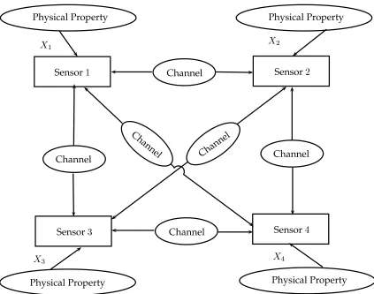
1.4 Mesh Topology . . . 5

1.5 Wireless sensor network protocol stack. [1] . . . 7

2.1 Distributed Detection . . . 22

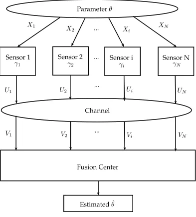
2.2 Distributed Estimation . . . 24

3.1 The model of a parallel sensor network under the attacks of an informed and greedy eavesdropper who eavesdrops on all the sensors decisions (i = 1. . . N) that are transmitted wirelessly via a binary symmetric channel with bit error rate ρE,i. The legitimate user receives sensor i data through another binary symmetric channel with bit error rate ρF,i < ρE,i.. . . 33

3.2 The maximum achievable detection performance trade-off un-der Neyman-Pearson framework using KLD for one sensor.. . . 52

3.3 The maximum achievable detection performance trade-off un-der Neyman-Pearson framework using KLD for one sensor.. . . 53

(D(¯α,β))

FC and at eavesdropper for N sensors. _DF and DE denote the actual KLDs at the FC and at eavesdropper, respectively. DfF and DEf denote the approximated KLDs at the FC and at

eavesdropper, respectively.. . . 54 3.5 When(α, β)_≈(1,1), the asymptotic secrecy and detection

per-formance using approximated and actual KLD(D(¯α,β¯))at the FC and at eavesdropper for N sensors. _DF and _DE denote the actual KLDs at the FC and at eavesdropper, respectively. DfF and DfE denote the approximated KLDs at the FC and at eavesdropper, respectively.. . . 55 3.6 ROC curves for the FC and eavesdropper with different

num-ber of sensors in N-P. The random guess line implies zero detectability. eavesdropper’s detectability is getting closer and closer to the diagonal line. . . 56 3.7 The maximum achievable detection performance trade-off

un-der Bayesian framework, where eavesdropper’s detection per-formance is constrained to the prior information.. . . 57 3.8 The asymptotic error exponent for the FC with ρF = 0 when

(α, β) _→ (0,0). As the number of sensor increases, the esti-mated error exponent approaches to the actual error exponent.58

NlnN e,F

number sensors increases, while Pe,E at eavesdropper is con-strained at π1. . . 59

4.1 Parallel sensor network model under eavesdropper attack, who eavesdrops on the output of sensor i, transmitted wire-lessly via a binary symmetric channel with bit error rate

ρE,i. The FC receives sensor i data through another binary

symmetric channel with bit error rate ρF,i < ρE,i.. . . 61 4.2 Total Fisher Information for the FC and eavesdropper with

different number of sensors given θ = 1, η = q4

3logN under

classical setting. As the number of sensors grow, the FI at the FC increases significantly while the FI at eavesdropper is close to zero. . . 73 4.3 Mean of estimated signal by the FC and eavesdropper with

different bit error rates under classical setting, where η =

q 4

3 logN, N = 100. The FC’s estimation is close to the ground

truth, while for eavesdropper, the estimations are off even the one with small bit error rate.. . . 74 4.4 MSE of estimated signals by the FC and eavesdroppers with

different bit error rates under classical setting, where the threshold, η=q4₃logN, N = 100. . . 75

the parameter, θ = 1 and the threshold, η=√logN. . . 76 4.6 Total Fisher Information for both the FC and eavesdropper

with different number of sensors under Bayesian framework, where η=√logN. . . 77

5.1 The maximum achievable KLD ratio for secrecy constrained distributed detection, ξF = 0 dB and ξE =−7 dB. . . 85 5.2 The actual KLD for the FC and eavesdropper with different

number of sensors, ξF = 0 dB and ξE =−7 dB. . . 86 5.3 The maximum KLD ratio for the FC and eavesdropper with

ξE =−7 dB. . . 87 5.4 The actual FI for secrecy constrained distributed estimation

with ξE =−7 dB, the number of sensors, N = 100.. . . 88

C.1 Operation Region is the inside area of two ROC curves.. . . 118

KLD – KullbackLeibler Divergence WSN –Wireless SensorNetwork FC –Fusion Center

IoT– Internet of Things LRT– Likelihood Ratio Test

ROC – ReceiverOperating Characteristic MSE– Mean Squared Error

CRLB – Cram´er RaoLower Bound LRQ –Likelihood Ratio Quantizer BER– Bit Error Rate

BSC – Binary SymmetricChannel SNR – Signal Noise Ratio

FI – Fisher Information

BPSK – Binary Phase Shifting Keying

α sensor false alarm probability

β sensor detection probability

η decision threshold

Pf false alarm probability at the decision center

Pd detection probability at the decision center

Pm missed detection probability at the decision center

TE prespecified performance threshold for Eve

TF prespecified performance threshold for the fusion center

Pe probability of error at the decision center

ρ bit error rate

γ decision rule

mean squared error

I Fisher information for one sensor I Fisher information for all sensors

D(P0(_·)_||P1(_·)) KLD for one sensor D(P0(·)||P1(·)) total KLD for all sensors

CHAPTER 1

INTRODUCTION

1.1

Wireless Sensor Networks

Comprised of a large number of low-cost, low-power, mobile and miniature sensors, wireless sensor networks (WSNs) are systems of detecting phenomena, estimating parameters or measuring some physical properties of the environment, where sensors are densely deployed to the region of interest [1, 5, 83, 88]. Many WSNs have a dedicated node called sink node or fusion center (FC), of which the computational capability is more powerful than other sensing nodes because of data fusion require-ments. Due to energy constraints, time-delay, bandwidth and memory limitations, the local nodes cannot send all the observed information directly to the FC where the final decision is made. The data observed by local sensors must be quantized or compressed before transmission over wireless channels to the FC. Therefore, one of the essential problems in WSNs is to design and optimize the local quantization rule for local nodes and fusion rule at the decision center in order to make the optimal inference at the FC based on the transmitted data from senors [5, 83, 88, 100].

1.1.1 Topologies in WSNs

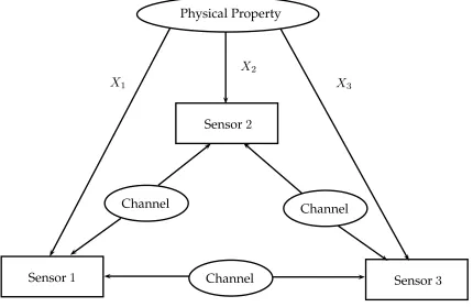
common topologies in WSNs include peer to peer networks, parallel (star) networks, tree networks, and mesh networks [72].

Physical Property

Sensor1 _Sensor3

X1 X3

Sensor2

X2

Channel _Channel

Channel

Figure 1.1: Peer-to-Peer Topology

In peer-to-peer network for three sensors shown in Figure 1.1, local sensors observe the physical property and they are able to send the outputs to each other across their respective channels. In this way, each sensor can be considered as the FC. Therefore, this network topology is flexible in a sense that when one sensor fails, another sensor could take over the job for decision making.

Physical Properties

Sensor 1

Sensor 2

...

Sensor N

X

_X

2

X

X

Channel

Fusion Center

...

γ

γ

γ

γ

Sensor i

...

Decision

...

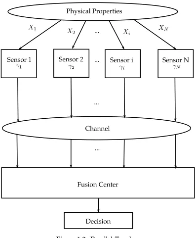
Figure 1.2: Parallel Topology

WSNs due to its simplicity and robustness. Under such a setting, the failure of a small portion of sensors will not deteriorate the performance of the network significantly.

Physical Properties

...

High level

Fusion Center ...

Decision

Mid level Low level

... ...

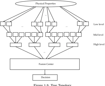
Figure 1.3: Tree Topology

level sensors observe the physical properties and then send their outputs to the next level and they keep doing so until the FC receives the output from high level nodes. This multi-hop communication is expected to consume less power than the single hop communication. Furthermore, the transmission power is low [97].

Physical Property

Sensor1

Sensor3

X1

X3

Sensor2

X2

Channel

Channel Channel

Sensor4

Channel

Chan

nel Cha

nne_l

Physical Property

Physical Property Physical Property

X4

Figure 1.4: Mesh Topology

most complicated structure.

To sum up, the characteristics of common topologies for WSNs are summarized in Table 1.1. The topology of a WSN does not necessarily remain the same because the sensors could be mobile and their locations may change from one place to another.

1.1.2 Sensors Communication Protocol

Table 1.1: Characteristics of Common Topologies for WSNs

Topology Name Advantages Disadvantages

Peer-to-Peer flexible not robust to sensor failures

Parallel

simple; robust in terms of sensor not flexible

failures and network performance

Tree

flexible; energy-efficient not robust to backbone

sensor failures

Mesh flexible; robust complicated

by sensor-to-sensor and sensor-to-FC. A protocol diagram is illustrated in Figure 1.5, which consists of the application layer, transport layer, network layer, data link layer, physical layer, power management plane, mobility management plane, and task management plane [1].

Each layer has their own functionalities and knows how to respond to the requests from the layer below or above. The main functions are summarized as follows:

• The application layer interacts with the end users and specifies how the data are requested.

Application Layer

Transport Layer

Network Layer

Data Link Layer

Physical Layer

Po

w

er

M

an

ag

em

en

t

M

ob

ilit

y

M

an

ag

em

en

t

Ta

sk

M

an

ag

em

en

t

Figure 1.5: Wireless sensor network protocol stack. [1]

• The network layer routes the incoming data to the desired locations.

• The data link layer is responsible for the multiplexing of data streams, data frame detection, medium access and error control.

• The physical layer is responsible for frequency selection, carrier frequency gen-eration, signal detection, modulation, and data encryption.

consumption and coordinate different tasks.

1.1.3 WSNs Applications

With topology and communication protocols in mind, the natural question is what kind of applications we can apply with WSNs. In fact, WSNs are widely employed in many applications such as environmental monitoring, cyber-physical systems, health-care, diagnostics of complex systems and military applications and so on. We sum-marize the main applications as the following categories.

• Environmental monitoring includes temperature monitoring (forest fire detec-tion), flood detection, geophysical research and so on [69, 76, 91]. Take forest fire detection as an example, where a large number of sensors are randomly and densely deployed to a forest in order to collect data on weather conditions including temperature, wind speed, rain and relative humidity. These sensors need to be durable in that they are often exposed to harsh environments. They send the compressed outputs to the FC through the wireless communication module, then the FC combines the information collected by local nodes and makes the final decision whether there is a fire or not in that forest [7].

power transmission lines in order to improve transmission efficiency, reliability and sustainability [26, 29].

• Health related applications include tracking patients’ physiological conditions, movements and behaviors. For this purpose, patients usually wear different types of wireless sensors to collect data on body conditions [31, 102]. For real-time applications such as telemonitoring of patients, sensors transmit to the FC securely in real-time. For offline decision-making, such as future medical diagnostics, drug administration in hospitals and so on, sensors collect data for a long time and then securely transmit the data to the FC.

• For complex systems like vehicles, airplanes or nuclear plants, WSNs keep monitoring the conditions of the parts, the environment or the function units, once the fault or anomaly occurs, the sensors would report to the FC [46, 50, 64]. One example for this application is a WSN deployed in an airplane cabin to monitor particulate matter, carbon dioxide, pressure and humidity to make sure the environment is suitable for passengers [35].

• Military applications include battlefield surveillance and reconnaissance of op-posing forces. WSNs can be deployed to detect, localize and track targets, moreover, they can be used to assess damage conditions, monitoring equipment and ammunition [62, 80].

sensor nodes in order to improve the overall quality of road transportations including safety, congestion, emissions, and traffic waiting time [23, 42, 51]. The Internet of things is another application of WSNs which aims at connecting home appliances, smart phones and other Internet connected devices [4] in order to improve energy-efficiency, convenience, safety and so on.

1.2

Cyber Attacks in WSNs

Wireless communication makes the aforementioned applications possible, on the other hand, wireless communication allows local nodes to broadcast and all of their wireless packets are potentially available to any other listeners. It also means WSNs are vulnerable to all kinds of attacks. As the data collected by the aforementioned applications could be extremely sensitive, care must be taken to prevent the collected information from being leaked to any malicious third parties. Thus, we need to understand the potential strategies of attackers against WSNs in order to defend them effectively.

In [92], Wang et al. surveyed cyber threats in sensor networks, which is summa-rized in Table 1.2. According to the security requirements in WSNs, these attacks can categorized as [73]:

• Secrecy and authentication attacks where eavesdroppers either passively listen to packets or modify packets in order to gain certain advantages.

• Stealthy attacks against service integrity where attackers falsify the data and make the network accept it so that the decision center is confused, e.g., Byzan-tine attackers.

Among all of these attacks, this dissertation concentrates on eavesdropping at-tacks in that it forms the basis or starting point for a large number of different, more malicious attack strategies. For example, if Byzantine attackers, jammers or intruders have reliable information provided by the eavesdropper, their subsequent attacks could be more efficient [65]. There are two types of eavesdropping attacks, passive and active. Passive eavesdroppers detect the information by tapping the data transmissions between the local sensors and the legitimate user; active eavesdroppers, however, send queries to some local sensors by disguising themselves as friendly nodes [20]. In this dissertation, we consider the general problem of passive eavesdropping because it is the foundation of active eavesdropping and it is difficult to detect and defend.

1.3

Cyber Defense Mechanisms

Table 1.2: Denial-of-service Attacks in WSNs[92]

Layer Attacks Defense

Physical

Jamming Spread-spectrum, priority messages, lower duty cycle, region mapping, mode change Tampering Tampering-proofing, hiding

Link

Collision Error-correcting code Exhaustion Rate limitation Unfairness Small frames

Network

Spoofed, altered Egress filtering, authentication, monitoring Selective

forward-ing

Redundancy, probing

Sinkhole Authentication, monitoring, redundancy Sybil Authentication, probing

Wormholes Authentication, packet leashes by using geo-graphic and temporal information

Hello food attacks Authentication, verify the bidirectional link Acknowledgement

spoofing

Authentication

Transport

1.3.1 Cryptography in WSNs

Cryptographic algorithms, which includes public key and symmetric key [37], have been widely used for computer networks where the nodes (computers) are powerful enough to implement the algorithms. However, due to the constraints in WSNs, where sensors are often operated on a limited battery power and limited computational power, many existing algorithms are not practical for use. Next, we discuss the feasibility of implementing the recent research on public key and symmetric key in WSNs.

Public Key Cryptography in WSNs

This asymmetric cryptography scheme uses pairs of keys: public keys which can be distributed widely, and private keys which are known only to the owner. Anyone can encrypt messages using the public key, however, only the owner of that paired private key can decrypt the message.

Symmetric Key Cryptography in WSNs

Unlike public key cryptography, symmetric key scheme uses the same cryptography keys for both encryption and decryption. The keys can be identical or a simple transformation applied between the two keys. This scheme consumes much less com-putational energy. In order to investigate the feasibility of symmetric key for WSNs, several popular algorithms including RC4 [56], RC5 [68], IDEA [56], SHA-1 [25] and MD5 [56, 66] were implemented on different microprocessors ranging in word size from 8-bit to 16-bit. The researchers compared the operation time and energy with these algorithms and they concluded that symmetric key cryptography is preferred in a WSN. The measurements on average execution time and energy consumption with different algorithms on Atmel ATmega128 processor are summarized in Table 1.3 and Table 1.4, respectively.

Table 1.3: Symmetric Key Cryptography: Average Execution Times on Atmel ATmega128[38]

Algorithm Operation Time (ms)

RC5 [68] 0.26ms

Table 1.4: Symmetric Key Cryptography: Average Energy Consumption on Atmel ATmega128[90]

Algorithm Energy

SHA-1 [25] 5.9 mJ/byte

AES-128 Enc/Dec [19] 1.62/2.49 mJ/byte

1.3.2 Physical-Layer Security Approach

Even though the symmetric key cryptography algorithms presented in section 1.3.1 consume low-power, they may not be low enough for long term WSNs operations, furthermore, they do require the devices to have the computational capability to per-form the required tasks which may not be true for some of the nodes [98]. Therefore, it is not always possible to completely rely on cryptographic techniques. Besides, key distribution brings another problem to WSNs, especially for dense WSNs. To address these issues, information-theoretic (physical-layer) security approaches, utilizing the characteristics of the physical layer, including transmission channels noises, and the information of the source, have gained considerable attention on this method to enhance the security, secrecy and privacy of WSNs [3, 55, 78, 103]. Additionally, physical-layer security for distributed detection is scalable due to the low computa-tional complexity [74]. Physical-layer security approaches can be used along with cryptosystems to further enhance WSNs and make the systems even more secure.

distributed detection against eavesdropping attacks for WSNs in parallel networks, where the goal was to maximize Kullback-Leibler Divergence (KLD) at the FC for one sensor, DF, under the constraint that KLD at an eavesdropper for one sensor, DE, is no more than a pre-specified threshold TE [58]. For a two-sensor network, where the attacker has the access to one of the sensors output, Li et al. jointly designed sensor decision rules and fusion rules to maximize the FC detection probability by constraining both the FC’s probability of false alarm and eavesdropper’s detection probability [48]. For privacy issues, Li and Oechtering formulated privacy-constrained and privacy-concerned optimization problems under Bayesian framework and derived the optimal privacy detection rule under a privacy guarantee constraint [47].

As for the secrecy constrained distributed estimation in WSNs, Aysal et al. pro-posed to solve the problem by adding a stochastic cipher as a security module, to randomly change the sensor outputs and disguise them from the eavesdropper [2]. Guo et al. considered using multiple-input multiple-output beamforming strategies to combat eavesdroppers, where local sensors use the analog amplify and forward scheme to communicate with the FC over a slow-fading orthogonal multiple access channel [28]. In [41], Khan and Stankovi´c proposed to securely estimate distributed data in cyber-physical systems by verifying statistical consistency on the nodal, local information and physical layer feedback.

cannot be directly employed under more general noisy channel models.

1.4

Contributions and Overview of the Thesis

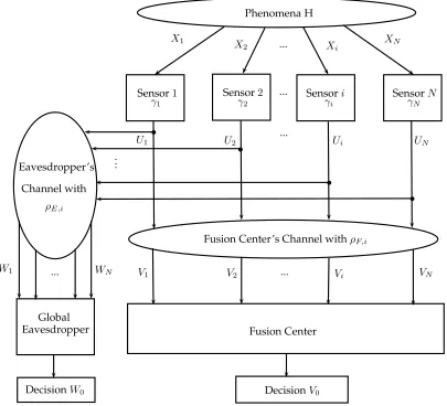
This dissertation focuses on using a physical-layer security approach to address the distributed inference problems with secrecy constraints in a sense that a WSN with parallel topology is eavesdropped by a global, greedy and informed eavesdropper, which has access to all the sensors outputs. The reason we consider parallel structure for WSNs lies in that it is simple and robust to sensor failures, when a small portion of sensor dies, the performance of the network would not be deteriorated. As a malicious user, this eavesdropper passively listens to the sensor outputs and aims at making informative decisions. However, the data collected by sensors are extremely sensitive, our goal is to prevent a malicious third party (eavesdropper) from stealing information from local nodes. Therefore, the ideal design for a sensor network is perfect secrecy where an eavesdropper does not obtain any useful information. We will discuss the possibility of (asymptotic) perfect secrecy. Moreover, we investigate performance trade-offs between the FC and eavesdropper, where the performance of the attacker is constrained to a level such that she could not make an informative inference; meanwhile, the performance of the legitimate user (FC) is guaranteed to perform well at the desired level. Utilizing the metrics of measuring secrecy in both detection and estimation problems, we provide results on the maximum achievable inference performance trade-off between the FC and eavesdropper.

This dissertation is organized as follows,

Chapter 2: Background and Fundamental Concepts

in the following chapters. The fundamental concepts include distributed detection, distributed estimation and secrecy metrics under different frameworks.

Chapter 3: Secrecy Constrained Distributed Detection in WSNs

We first investigate detection problems under secrecy constraints. The main contributions of secrecy constrained distributed detection in WSNs are summarized as follows:

1. Analyze the detection performance at the FC and eavesdropper, respectively. For the case where the sensor outputs are binary, we evaluate the quality of the received sensor decisions when the sensors employ likelihood ratio quantizer (LRQ) close to the extreme points on receiver operating characteristics (ROC) curve.

2. Utilizing performance analysis, we propose a novel approach of analyzing the performance trade-off between the FC and eavesdropper using the maximum achievable detection performance ratio between the FC and eavesdropper, given both a noise free and noisy FC channel. Additionally, we show that both asymptotic perfect secrecy and asymptotic perfect detection are possible by increasing the number of sensors when the FC has noiseless channels under the Neyman-Pearson framework.

perfect detection are possible. The results contradict the idea that network security tends to decrease as the number of sensors increases.

Chapter 4: Secrecy Constrained Distributed Estimation in WSNs

In this chapter, we investigate the secrecy constrained distributed estimation problem and the main contributions are summarized as follows:

1. Under classical settings, where the parameter to be estimated is fixed but unknown, we analyze the estimation performance at the FC and eavesdropper using Fisher information, respectively. In order to investigate the possibility of perfect secrecy, we propose the Fisher information ratio between the FC and eavesdropper. Furthermore, for Gaussian noise, we show how to design the threshold in order to achieve asymptotic perfect secrecy and asymptotic perfect estimation.

2. Under the Bayesian framework, where the parameter is a random variable, we analyze the performance trade-off between the FC and eavesdropper using Fisher information and show that the secrecy constraints can be satisfied for both the FC and eavesdropper under Gaussian noise case.

Chapter 5: Secrecy Constrained Distributed Inference with Parallel Fading Binary Symmetric Channel Models

CHAPTER 2

BACKGROUND AND BASIC CONCEPTS

2.1

Statistical Inference

In the classical statistical inference, all the data is collected and processed in a centralized fashion. Distributed inference, however, detects signal presence, estimates parameters and tracks targets based on distributed data from local sensors [83, 86]. It has been the focus of multiple disciplinary research in the past several decades [6, 10–12, 81, 85, 89]. One of the essential problems in distributed inference is to optimize decision-making at the information center by the design of local decision sensor rules for each sensor and global decision rules at an information center [83]. Without constraints on “distributed” settings, the problems of inference share much in common with many centralized statistical inference and learning problems such as signal detection and estimation, dimension reduction and feature extraction [60]. Due to the additional condition on “distributed”, the complexity of the inference problem is increased significantly [82].

phenomenon is often a parameter in a continuous set [36]. In the following sections, we introduce the basic settings in distributed detection and distributed estimation.

2.2

Distributed Detection

Hypotheses

H

Sensor 1

Sensor 2

...

Sensor N

X

_X

2

X

X

Channel

Fusion Center

...

γ

γ

γ

γ

Sensor i

...

Decision

...

U

U

U

U

V

V

V

V

V

As one of the essential aspects of distributed inference, distributed detection is often the initial goal of a pattern recognition system and aims at detecting signals or events as accurately as possible [86] with the distributed data collected by various sensors, where the data can be generated from the underlying binary or M-ary hypotheses. Distributed detection can be widely used for both military and civilian applications including distributed array radar, intruder detection, anomaly detection and intelligent transportation system where the infrastructure sensors detect pedes-trians, vehicles and anomaly events [23, 42, 51]. For instance, N sensors are densely deployed in forests to observe the temperatures, and through a channel, these nodes send the quantized outputs to the FC where the final decision is made about whether there is forest fire or not [69]. For WSNs, detecting the presence of an event is the priority of all the other tasks including estimation, tracking and learning [11]. Hence, as a key function in WSNs, distributed detection has been an important and active research area over the past several decades [6, 10–12, 14, 77, 81, 85, 89].

In Figure 2.1, we show the structure of distributed detection in a parallel WSN, where local sensors observe the hypothesesH and obtain their dataXi, (i= 1. . . N). With the decision rules for each sensor,γi, sensoricompresses the data to the outputs

Ui, which is transmitted across a channel. In the end, the FC makes the decision V0

based on the received Vis, the output of channels from the input Uis.

2.3

Distributed Estimation

Parameter

θ

Sensor 1

Sensor 2

...

Sensor N

X

_X

2

X

X

Channel

Fusion Center

...

γ

γ

γ

γ

Sensor i

...

Estimated

_θ

ˆ

...

U

U

U

U

V

V

V

V

Figure 2.2: Distributed Estimation

system, the following task would be estimating how fast the vehicle is moving and where it is moving.

Similar to the distributed detection setting, in Figure 2.2, we present the structure of distributed estimation, where sensors observe a scalar or vector parameterθ, sensors quantized outputs Ui (i = 1. . . N) are sent to the FC through a channel. Then the parameter ˆθ is estimated at the FC based upon received Vi.

2.4

Performance and Secrecy Metrics

From the aforementioned applications about distributed detection and distributed estimation, we can see that the information collected by the systems is very sensitive and care must be taken to prevent them from being leaked to any malicious third parties. Hence, we focus on secrecy constrained inference in WSNs where the ultimate goals are restricting the ability of eavesdropping from attackers and maintaining high performance at the FC. Hence, we first introduce secrecy.

Secrecy in WSNs against eavesdropping attacks means that any malicious listeners should not be able to make informative decisions based on messages from local sensors that are supposed to go to the FC. In other words, in distributed inference, secrecy measures the inference performance at the FC and eavesdropper respectively. For instance, if the inference performance at the FC is higher than the specified level while eavesdropper’s performance is lower than a random guess, the WSN is considered as secure in terms of secrecy. For this purpose, we introduce the performance metrics for distributed detection and distributed estimation, respectively, in this section.

2.4.1 Distributed Detection under Neyman-Pearson Framework: Infor-mation Divergence

maps the dissimilarity between two probability distributions to nonnegative values. It is also extended to machine learning problems where the goal is to minimize the approximation error between the observed data and the approximated model [22]. There are several information divergences and they are summarized in Table 2.1, where x > 0 is the observed data and µ is the approximation given by the model. Forγ-divergence and R´enyi-divergence, the input data needs to be normalized, where ˜

xi =xi/

P

jxj and ˜µi =µi/

P

jµj.

Since there are so many choices of information divergence, which one should we consider? According to Stein’s lemma [12] and large deviation theory [8, 16], when the decision center observations are i.i.d., the error exponent of probability of missed detection (Pm) is bounded, a special case ofγ-divergence, Kullback-Leibler divergence (KLD),D(p0(·)||p1(·)), wherep0, p1 are the pdf underH0 andH1 hypotheses, respec-tively. Specifically,− lim

N→∞

1

N logPm ≤D(p0(·)||p1(·)) (N is the number of sensors in a WSN) when the false alarm probability (Pf) is constrained to be less than a constant, and the equality can be achieved by the optimal LRT or other asymptotic optimal detectors such as type based detectors so that [18],

Pm ≈e−N D(p0(·)||p1(·)). (2.1)

For binary sensor decisions with P(Ui = 1;H0) = α and P(Ui = 1;H1) = β, we haveP(Ui = 0;H0) = 1−α andP(Ui = 0;H1) = 1−β, the KLD [44] for each sensor is

D(p0||p1) =αlog α

β + (1−α) log

(1₋α)

(1−β) =D(α, β). (2.2)

Pf ≈e−N D(p1(·)||p0(·)). (2.3)

The corresponding KLD is

D(p1||p0) =βlog β

α + (1−β) log

(1−β)

(1₋α) =D(β, α). (2.4)

2.4.2 Distributed Detection under Bayesian Framework: Probability of Error

Under Bayesian framework, prior information needs to be taken into consideration. Let the risk functionλ(ai|Hj) be the risk or loss incurred for taking actionaiwhen the actual hypothesis is Hj, wherei∈[0, . . . , N], and N indicate the number of possible actions, and j ∈[0, . . . , C],C is the number of states of nature (categories) [24]. The overall risk is

r = N

X

i=0

C

X

j=0

λ(ai|Hj)P(ai|Hj)P(Hj),

whereP(ai|Hj) is the probability of actionigiven the state of natureHj,P(Hj) is the probability of category Hj. For C = 1, two-category case, to simplify the notation, letλij =λ(ai|Hj),P(Hj) =Pj and the actions be,

a0 : decide H0 a1 : decide H1

Table 2.1: Information Divergence[22]

Name Definition Special Cases

α-divergence

Dα(x||µ)

P

ixαiµ

1−α

i −αxi+(α−1)µi α(α−1)

Dα=2(x||µ) = 1₂ Pi

(xi−µi)2 µi

Dα→1(x||µ) = Pi

xilnx_µi

i −xi+µi

Dα=1

2 (x||µ) = 2

P

i √_x

i−√µi

2

Dα→0(x||µ) = Pi

µilnµ_xi_i −µi+xi

Dα=−1(x||µ) = ₂1 P_i (xi−µi)

2

xi

β-divergence

Dβ(x||µ)

P

ix β+1

i +βµβ+1−(β+1)xiµβi β(β+1)

Dβ=1(x||µ) = 1₂Pi(xi−µi)2

Dβ→0(x||µ) =Pi

xiln_µxi_i −xi+µi

Dβ→−1(x||µ) =P_i

xi µi −ln

xii µi −1

Dβ=−2(x||µ) =Pi

xi

2µ2

i −

1

µi +

1 2xi

γ-divergence

Dγ(x||µ)

1

γ(1 +γ)ln

X

i

xγi+1

!

+ 1

(1 +γ)ln

X

i

µγi+1

!

− 1

γ ln X

i

xiµγi

!

Dγ→0(˜x||µ˜) = Pix˜iln

˜

xi

˜

µi

R´enyi-divergence

Dρ(x||µ)

1

ρ−1ln P

ix˜ p iµ˜

1−p i

where ˜xi = xi/

P

jxj, ˜

µi =µi/

P

r =λ00P (decide H0|H0)P0 +λ01P (decide H0|H1)P1+

λ10P (decide H1|H0)P0+λ11P (decide H1|H1)P1

=λ00(1₋Pf)P0+λ01PmP1+λ10PfP0+λ11(1−Pm)P1 =λ00P0+λ11P1+ (λ10−λ00)PfP0 + (λ01−λ11)PmP1

Since λ00P1 and λ11P0 are constant, we can put them aside. Therefore, the overall risk function is reduced to

r = (λ10₋λ00)PfP0+ (λ01−λ11)PmP1

Then we normalize r by

r

(λ10₋λ00)P0+ (λ01₋λ11)P1 =

(λ10−λ00)P0

(λ10₋λ00)P0+ (λ01₋λ11)P1Pf

+ (λ01−λ11)P1

(λ10−λ00)P0+ (λ01−λ11)P1 Pm

Let

π0 = (λ10−λ00)P0

(λ10₋λ00)P0+ (λ01₋λ11)P1

π1 = (λ01−λ11)P1

(λ10−λ00)P0+ (λ01−λ11)P1 ,

we have

Pe =π0Pf +π1Pm (2.5)

2.4.3 Distributed Estimation under Classical Setting: Mean Squared Er-ror and Fisher Information

For estimation problems under a classical setting, a natural criterion for evaluating the performance is the mean squared error (MSE), which is defined in Equation (2.6).

MSE =Eθˆ−θ2 (2.6)

where, θ is a scalar parameter and ˆθ is the estimated parameter. We will use MSE evaluation as the performance metric when feasible.

However, sometimes computing MSE is not straightforward and even intractable for some cases. Instead, Cram´er-Rao lower bound (CRLB) [39, 79] is often used which is equivalent to evaluating the Fisher information (FI),

I(V;θ),EV

∂2_logp(V;θ) ∂2_θ

(2.7)

where V is the data transmitted from local sensors across the channel (Figure 2.2),

p(V;θ) is probability density function (PDF) of parameter θ given V [39]. And the MSE is bounded away from CRLB for scalar parameter θ is,

MSE_≥CRLB(V;θ) = 1 I(V;θ).

2.4.4 Distributed Estimation under Bayesian Setting: Bayesian Cram´ er-Rao Lower Bound

MSE_≥BCRLBF (V;θ) = (I(V;θ))−1 =

Z ∞

−∞

N I(η, θ, ρF)p(θ)dθ+I(λ)

−1

(2.8) where

I(λ) =

Z

∂logp(θ)

∂θ 2

p(θ)dθ,

and V is the same with the one defined in (2.7) and p(θ) is the prior density about the random variableθ.

CHAPTER 3

SECRECY CONSTRAINED DISTRIBUTED DETECTION

IN WSNS

This chapter is organized as follows. In Section 3.1 and Section 3.2, we introduce the system model, detection performance metric, and set the secrecy constraints under both frameworks in WSNs, respectively. In Section 3.3, we solve the secrecy constrained problem under Neyman-Pearson framework and explain how to achieve asymptotic perfect secrecy in detection. We then analyze the secrecy constrained distributed detection problem under the Bayesian framework in Section 3.4. In Section 3.5, we provide simulation results to further support our proofs.

3.1

Distributed Detection in Sensor Networks

3.1.1 WSN Model

We consider a distributed detection problem with binary hypotheses, H0 and H1, in

a parallel WSN as shown in Figure 3.1. The key components of our research problem are described as follows:

Phenomena H

Sensor1 Sensor2

...

SensorN

X1 _X

2 Xi XN

U1 U2 Ui UN

Fusion Center’s Channel withρF,i

Fusion Center Eavesdropper’s

Channel with

ρE,i

Global

...

γ1 γ2 γi γN

Sensori

...

...

... ...

Eavesdropper

DecisionW0 DecisionV0

W1 WN _{V1 V2 Vi VN}

Figure 3.1: The model of a parallel sensor network under the attacks of an informed and greedy eavesdropper who eavesdrops on all the sensors de-cisions (i= 1. . . N) that are transmitted wirelessly via a binary symmetric channel with bit error rate ρE,i. The legitimate user receives sensor i data through another binary symmetric channel with bit error rate ρF,i< ρE,i.

the parallel structure can still be carried out virtually by leaving relay nodes to forward all sensor outputs.

at sensor i, respectively, where k = 0,1 and i = 1,2, . . . , N. We assume that

p0(Xi) and p1(Xi) are continuous pdfs with no point mass. The log-likelihood ratio ln (p1(Xi)/p0(Xi)) is assumed to be unbounded. Sensor i makes a binary decision Ui ∈ {0,1} based on its decision rule γi, such that P(Ui = 1|Xi) =

γi(Xi)∈[0,1], ∀i.

3. Channel model. The communication channel between sensor i and its target receiver is assumed to be a binary symmetric channel (BSC), a channel model widely employed in SN communications for binary coding schemes such as binary phase-shift keying (BPSK) [45, 71, 101]. This model also serves as a good starting point to study other more complicated channel models. Sensor i

sends its quantized output Ui to the FC over a BSC with bit error rate (BER)

ρF,i < 1₂, with a received decision,Vi.

4. Attack model. All of the sensors outputs are eavesdropped by Eve via a set of parallel wiretapping channels. Eve receives Wi (i= 1, . . . , N), from sensor

i as an output of a BSC channel with BER ρE,i < 1₂. We assume that Eve’s channel is noisier than the FC’s such thatρE,i > ρF,i, which can be achieved by using directional antennas to improve the FC SNR, resulting in a lower BER [52, 75, 99]. Note, an analysis similar to what follows can be employed for different channel models. Other than receiving a set of different observations W = [W1, . . . , WN], Eve is assumed to have the same information about the detection algorithm as the FC does, including the sensor observation model, sensor decision rule, channel status and the prior probabilities of hypotheses,

P(H0) = π0 and P(H1) =π1.

sensors observations and the communication channels are conditionally inde-pendent and identically distributed (i.i.d.). Specifically,

p(X1, X2, . . . , XN;Hj) = N

Y

i=1

p(Xi;Hj), j = 0,1,

for the sensor observations, and ρE = ρE,i with ρF = ρF,i for all i for the communication channels.

3.1.2 Received Decision Qualities

For its simplicity and robustness, we employ identical sensor design in this chapter. That is, the decision rule γi(_·) at sensor i is a likelihood ratio quantizer such that

γi(x) = γ(x) =

              

1 p1(x)

p0(x) ≥η

0 p1(x)

p0(x) < η.

(3.1)

Under the conditional i.i.d. assumption, it has been shown that the identical sensor decision rule design, where each sensor uses the same likelihood ratio test (LRT) with the same threshold, is at least asymptotically optimal at the FC (i.e., no eavesdropper) [17, 81, 93].

At the ith local sensor, the resulting probability of false alarm αi, and the proba-bility of detection βi are given by [84]

αi =P(Ui = 1|H0) = P

p1(Xi)

p0(Xi) ≥ η_|H0

βi =P(Ui = 1|H1) = P

p1(Xi)

p0(Xi) ≥η|H1

.

and

dβi

dαi

=η. (3.2)

Therefore, since ln (p1(Xi)/p0(Xi)) is unbounded, then η → ∞ as αi, βi → 0, or

η _→ 0 as αi, βi → 1. Because of the i.i.d. assumption on the observations, decision rules and channels, we have

α =α1 =α2_{· · ·}=αN

β =β1 =β2· · ·=βN.

Due to the binary symmetric channel between the local sensors and the FC, the received decision, Vi, from sensor i at the FC, has the following performance,

P(Vi = 1|H0) =αF =α(1−ρF) + (1−α)ρF =ρF + (1−2ρF)α,

P(Vi = 1|H1) =βF =β(1−ρF) + (1−β)ρF =ρF + (1−2ρF)β.

(3.3)

P(Wi = 1|H0) = αE =ρE + (1−2ρE)α,

P(Wi = 1|H1) =βE =ρE + (1−2ρE)β.

(3.4)

3.2

Secrecy in Distributed Detection

With the model of the WSN, we introduce the performance metrics that lead to secrecy constraints in distributed detection under both frameworks. The first perfor-mance metric applicable under the Neyman-Pearson framework is the KLD.

3.2.1 Performance Metric and Secrecy Constraints under Neyman-Pearson framework

When the decision center’s observations are i.i.d. and the probability of false alarm,

Pf = (decide H1|H0), is constrained to be no greater than a fixed constant, it is known that the error exponent of the probability of missed-detection, Pm = (decide H0|H1), is bounded by the corresponding KLD, D(p0(_·)_||p1(_·)) [44], between the p0, the pdf under H0, and p1, the pdf under H1, such that [8, 12, 16]

− lim N→∞

1

N lnPm ≤D(p0(·)||p1(·)) =Ep0(·)

dp0(·)

dp1(_·)

(3.5)

Notice that equality in (3.5) can be achieved via optimal LRT detectors or other asymptotically optimal detectors such as type based detectors [18]. Similarly,D(p1(_·)_||p0(_·)) is the error exponent rate forPf whenPm is constrained to be no more than a certain threshold.

D α,¯ β¯

,α¯lnα¯_¯

β + (1−α¯) ln

1−α¯

1−β¯, (3.6)

where ¯α and ¯β are generic notations of probability of false alarm and probability of detection, respectively, for both the FC and eavesdropper.

The KLD is always non-negative and equals 0 if and only if ¯α = ¯β. Similarly, for a boundedPm, the error exponent ofPf decays exponentialy in the number of sensors at the rate of D β,¯ α¯

such that Pf ∝e−N D( ¯β,α¯), where,

D β,¯ α¯

,β¯lnβ¯ ¯

α + 1−β¯

ln1−β¯

1₋α¯. (3.7)

For example, the KLD of each received sensor decision Vi at the FC is Di(αF, βF) withαF,βF defined in Equation (3.3) and KLD of each received sensor decisionsWiat the eavesdropper isDi(αE, βE). Owing to i.i.d. condition,Di(αF, βF) =D(αF, βF),

Di(αE, βE) =D(αE, βE), and the KLD at the FC and at eavesdropper for allN are,

DF = N

X

i=1

Di(αF, βF) = N D(αF, βF),

DE = N

X

i=1

Di(αE, βE) =N D(αE, βE),

(3.8)

respectively.

The detection performance in terms of the probability of missed-detection at the FC and at eavesdropper decays exponentially such that

and

Pm,E ∝e−DE.

Therefore, to limit eavesdropper’s detectability, one needs to make _DE as small as possible, and DF as large as possible, to maximize the FC detection performance, which leads to the following secrecy constraints.

Secrecy Constraints under the Neyman-Pearson framework

   

  

DE =N D(αE, βE)≤TE, DF =N D(αF, βF)≥TF,

(3.9)

where TE and TF are the KLD thresholds for eavesdropper and the FC, respectively, and DE and DF are defined in Equation (3.8).

• Feasibility: Is it possible to design a sensor network for the targeted TE and

TF?

• Secrecy and detection trade-off: minimize TE under fixed TF or maximize

TF under fixed TE. For non-asymptotic cases, we want the detectability at eavesdropper to be as low as possible and the detection performance at the FC to be as high as possible. However, in practice, a performance trade-off between the FC and eavesdropper must be considered.

• Asymptotic perfect secrecy: TE → 0 as the number of sensors, N → ∞, for example, TE ∝ N−µ, 0 < µ < 1. In this case, eavesdropper’s detection capability diminishes asN increases.

3.2.2 Performance Metric and Secrecy Constraints under Bayesian frame-work

To measure the detection performance under Bayesian framework, we consider the overall probability of error, Pe,

Pe =π0Pf +π1Pm, (3.10)

where π0 and π1 = 1−π0 are known to both the FC and an informed and greedy eavesdropper. Without loss of generality, we assume π1 ≤ 1

2 ≤π0, which is known by

both the FC and eavesdropper. Note, π0 and π1 = 1−π0 are the prior probabilities

of H0 and H1, respectively.

Thus, for the binary hypotheses testing problem secrecy constraint, the goal is to minimize the probability of error at the FC and to increase the Pe at eavesdropper as much as possible. We formulate the optimization problem as follows:

Secrecy Constraints under Bayesian framework

   

  

Pe,E ≥ΘE

Pe,F ≤ΘF,

(3.11)

where Pe,E and Pe,F are the probability of error for eavesdropper and the FC respec-tively, and ΘE and ΘF are the probability of error thresholds for eavesdropper and the FC, respectively.

• Asymptotic perfect secrecy: ΘE → min(π0, π1) =π1 and Pe,E →min(π0, π1) =

π1 as N → ∞. In this case, observations do not provide any useful or critical information and all that eavesdropper can do is rely on the prior information and decide H0 regardless of any Wi. Similar to the perfect secrecy constraint, as the number of sensors increases, eavesdropper receives vanishingly useful information from the observations.

• Asymptotic perfect detection: ΘF _→0 as N _{→ ∞}.

Knowing the secrecy definition and constraints, we will now solve the optimization problems in the following sections.

3.3

Performance Analysis Under Neyman-Pearson

Frame-work

3.3.1 Maximum Achievable Performance

Table 3.1: Approximated KLD

(α, β)≈(0,0) (α, β)≈(1,1)

¯

ρ= 0

D(¯α,β¯) β (1₋α)ln1−α

1−β −1

D( ¯β,α¯) β lnβ α −1

1₋α

¯

ρ >0

D(¯α,β¯) 1 2

β2_(1−2¯ρ)2

(1−ρ¯)¯ρ

1 2

(1−α)2_(1−2¯ρ)2

(1−ρ¯)¯ρ

D( ¯β,α¯) 1₂β2₍₁(1₋−_ρ¯2¯_)¯ρ_ρ)2 1₂(1−α₍₁)2₋(1_ρ¯)¯−_ρ2¯ρ)2

3.3.2 Noiseless Channel at the FC, where, ρE >0 and ρF = 0

Based on the defined secrecy constraints and Table 3.1, we investigate two different scenarios for the FC; one is when the channel is perfect, the other is with an imperfect channel.

For N i.i.d sensors with total KLD at eavesdropper is constrained atTE by,

DE =N D(αE, βE) = TE. (3.12) SinceρE 6= 0 and from Equation (A.3), we approximate the threshold at eavesdropper,

N

2

β2_(1−2ρE)2

(1₋ρE)ρE ≈

TE.

Therefore, at all the sensors, the operating point should be

β≈

s

2TE(1−ρE)ρE

which indeed goes to 0 as TE/N → 0. Because ρF = 0, from Equation (3.3) and (A.4), it can be shown that the per sensor KLD is

D(αF, βF)≈β ≈

s

2TE(1−ρE)ρE

N(1₋2ρE)2 , and the total KLD is

DF =N D(αF, βF)≈N β ≈

s

2N TE(1−ρE)ρE (1−2ρE)2 .

(3.14)

This can be utilized to design the secrecy against eavesdropper and the detection performance at the FC. For example, if we let TE beN−µ, (0< µ <1), which results inβ _≈q2N−µ(1−ρE)ρE

N(1−2ρE)2 , then

DF ≈N

1−µ

2

s

2 (1₋ρE)ρE (1−2ρE)2

.

Therefore, the performance and secrecy of the SN improves as the increment of the number of sensors, N, such that,

      

DE ∝N−µ

DF ∝N

1−µ

2 ,

(3.15)

perfect secrecy. We summarize the findings in the following theorem.

Theorem 1. Asymptotic Perfect Secrecy and Asymptotic Perfect Detec-tion under Neyman-Pearson Framework: When eavesdropper has a noisy channel, ρE >0, and the FC has a noiseless channel, ρF = 0, the secrecy constraints

(_{DE ≤}TE; DF ≥TF) can be satisfied for any arbitrary constants TE and TF, given a

sufficiently large number of sensors, N.

3.3.3 Noisy Channel, where, ρF >0 and ρE >0

Rarely does a perfect communication channel exist in practice, so we investigate the case where the FC has a noisy channel. Since ρF 6= 0, from Table 3.1, we know that

D(αF, βF)≈ 1 2

β2_(1−2ρ

E)2 (1₋ρE)ρE

.

Under the secrecy constraint in Equation (3.9), after applyingβfrom Equation (3.13), we obtain

DF ≈ TEρE(1−ρE)(1−2ρF)

2

ρF(1−ρF)(1−2ρE)2

. (3.16)

To measure the performance trade-off, we define the KLD ratio between the FC and eavesdropper as,

R = DF DE =

D(αF, βF)

D(αE, βE)

= D(βF, αF)

D(βE, αE)

(3.17)

Therefore, if we plug Equation (3.16) into Equation (3.17), we have the following result for the performance trade-off between the FC and eavesdropper.

ρF >0 and ρE > 0, the secrecy constraints can only be achieved for certain TE and

TF such that TF/TE is no more than the ratio, R = (1 −ρE)ρE

(1−ρF)ρF

1−2ρF

1−2ρE

2

.

(See Appendix B for the detailed proof).

For example, if ρF = 0.1,ρE = 0.3, and the required DF >10, the resulting infor-mation leakage isDE >1.07. In other words, the information leakage is inevitable, no matter how one increases the number of sensors in the network. On the other hand, when ρF is much smaller than ρE by using the techniques mentioned in [32–34, 99], then the performance ratio can still be large enough to maintain high detectability at the FC and poor performance at eavesdropper. This point is expanded upon in Section 3.5. The ratio can also serve as a performance design protocol for the SN, for instance, the desired performance at the FC and at eavesdropper are TF and TE, we can compute the correspondingρF when ρE is fixed or the other way round.

3.4

Performance Analysis Under Bayesian Framework

Recall that the goal under Bayesian framework is to minimize the probability of error in Equation (3.10) at the FC and constrain that at eavesdropper at a certain level.

3.4.1 Detection Performance Trade-off under Perfect Secrecy Constraint

Since both the FC and eavesdropper know the exact prior probabilities and π0 ≥π1,

the detection eavesdroppers probability of error bound is π1 achieved by accepting

P(H1_|W)_≤P(H0_|W), _∀Wi =⇒P(W|H1)π1 ≤P(W|H0)π0, ∀Wi =⇒ p(W|H1)

p(W_|H0) ≤

π0 π1 ∀Wi

=⇒ argmax W

p(W_|H1) p(W|H0)

≤ π0

π1 ∀Wi.

The maximum of the LRT is achieved when W1 = W2 = _{· · ·} = WN = 1 such that maxp(W|H1)

p(W|H0)

= (βE/αE) N

with αE and βE defined in Equation (3.4). That is, in order to limit eavesdropper’s detectability to the prior information,

βE

αE

N

≤ π0

π1. (3.18)

In this case, the wirelessly tapped sensors observations can provide some information, but not enough to overcome the prior information to make any difference in the final decision making.

Meanwhile, for the performance at the FC, we derive the following theorem,

Theorem 3. Maximum Achievable Performance Trade-off under Bayesian Framework When the FC has a noiseless channel and eavesdropper has a noisy channel, 0 < ρE < 0.5, the minimum achievable Pe,F at the FC is given by , limN→∞Pe,F =Pfπ0 =π1

π0

π1

−₁₋ρE_2ρE

.

Pe,F is a function of prior probabilities and the eavesdropper’s channel qualities

Remark 1. When π0 = π1 = 0.5, then Pe,F = 0.5, that means, it is impossible to achieve perfect secrecy, while providing the FC with any useful information.

For the case that the FC does not have a perfect channel, where ρF > 0, the detection performance becomes worse, and the corresponding probability of error at the FC increases as well.

3.4.2 Asymptotic Perfect Secrecy and Asymptotic Perfect Detection

We know that asymptotic perfect secrecy and asymptotic perfect detection can be achieved under N-P framework from Theorem 1, here we investigate the same problem under the Bayesian framework, requiring

Pe,E →min (π0, π1), N → ∞.

To evaluate the asymptotic error rate, we need to establish the error decay rate bound for the FC and eavesdropper respectively. First, from large deviation theory, for any decision center with conditionally i.i.d., Bernoulli observationsYi withP(Yi = 1_|H0) = ¯α and P(Yi = 1|H1) = ¯β, i= 1,2, . . . , N, the decision rule is

PN

i=1Yi

N

H1

≷

H0

T.

Based on the work in [16] and the Chernoff inequality

Pf ≈e−N D(T ,α¯),

Pm ≈e−N D(T ,

¯

β)_,

max (lnPf + lnπ0, lnPm+ lnπ1)≤lnPe, lnPe≤max (lnPf + lnπ0, lnPm+ lnπ1) + ln 2.

(3.19)

Hence, for a sufficiently large N,

−lnPe

N ≈min

−lnPf

N ,−

lnPm

N

,

≈min D(T,α¯), D(T,β¯) .

(3.20)

Therefore, the optimal T for large N is chosen such that D(T,α¯) = D(T,β¯). In Appendix D, we show that

T = D(¯α,β¯) ¯β+D( ¯β,α¯)¯α

D( ¯β,α¯) +D(¯α,β¯) , (3.21) which reveals the relationship betweenT and the KLD distancesD(¯α,β¯) andD( ¯β,α¯).

Table 3.2: Decision Rule ThresholdT

(α, β)≈(0,0) (α, β)≈(1,1)

¯

ρ= 0 β−α

lnβ_α +α β+

α−β

ln1₁−α_−β

¯

By plugging the decision rule threshold into the approximated KLD in Table 3.1, we summarize the approximated asymptotic error exponent in Table 3.3.

Table 3.3: Approximated Asymptotic Error Exponent

(α, β)≈(0,0) (α, β)≈(1,1)

¯

ρ= 0 β−α

ln_αβ +α

lnβ−α αlnβ_α

1₋β_−lnα−1−αβ

1−β

ln

α−β

(1−β) ln1−α

1−β

¯

ρ >0 1₈β2₍₁(1₋−_ρ¯2¯_)¯ρ_ρ)2 1₈(1−α₍₁)₋2(1_ρ¯)¯−_ρ2¯ρ)2

According to Table 3.3, when (α, β)→(0,0) andρF >0, the asymptotic error rate at FC can be approximated as β2(1−2ρF)2

8ρF(1−ρF). Similarly, for eavesdropper with ρE > 0, the error exponent D(TE, αE) = D(TE, βE) ≈ β

2_(1−2ρ

E)2

8ρE(1−ρE). Since Pe,E ∝ e

−N D(TE,βE)_, in order to achieve the asymptotic perfect secrecy under the Bayesian settings, it is required that

N β2(1₋2ρE)2 →0, N → ∞ =⇒ β =o

√

N−1_{, (3.22)}

wheref =o(g) denotes that functionf grows strictly slower than functiong, whereas

f =O(g) meansf grows slower than or equal tog.

Meanwhile, when the FC channel is noise free and (α, β) _→ (0,0), we have

TF = β_ln−βα α

+α and the resulting asymptotic error exponent D(TF, α) = D(TF, β) ≈

β−α

lnβ_α +α

ln β−α αlnβ_α