R E S E A R C H A R T I C L E
Open Access
Statistical power as a function of Cronbach
alpha of instrument questionnaire items
Moonseong Heo
1*, Namhee Kim
2and Myles S. Faith
3Abstract
Background:In countless number of clinical trials, measurements of outcomes rely on instrument questionnaire items which however often suffer measurement error problems which in turn affect statistical power of study designs. The Cronbach alpha or coefficient alpha, here denoted byCα, can be used as a measure of internal consistency of parallel instrument items that are developed to measure a target unidimensional outcome construct. Scale score for the target construct is often represented by the sum of the item scores. However, power functions based onCαhave been lacking for various study designs.
Methods:We formulate a statistical model for parallel items to derive power functions as a function ofCαunder several
study designs. To this end, we assume fixed true score variance assumption as opposed to usual fixed total variance assumption. That assumption is critical and practically relevant to show that smaller measurement errors are inversely associated with higher inter-item correlations, and thus that greaterCαis associated with greater statistical power. We
compare the derived theoretical statistical power with empirical power obtained through Monte Carlo simulations for the following comparisons: one-sample comparison of pre- and post-treatment mean differences, two-sample comparison of pre-post mean differences between groups, and two-sample comparison of mean differences between groups. Results:It is shown thatCαis the same as a test-retest correlation of the scale scores of parallel items, which enables testing significance ofCα. Closed-form power functions and samples size determination formulas are derived in terms ofCα, for all of the aforementioned comparisons. Power functions are shown to be an increasing function ofCα, regardless of comparison of interest. The derived power functions are well validated by simulation studies that show that the magnitudes of theoretical power are virtually identical to those of the empirical power.
Conclusion:Regardless of research designs or settings, in order to increase statistical power, development and use of instruments with greaterCα, or equivalently with greater inter-item correlations, is crucial for trials that intend to use
questionnaire items for measuring research outcomes.
Discussion:Further development of the power functions for binary or ordinal item scores and under more general item correlation strutures reflecting more real world situations would be a valuable future study.
Keywords:Cronbach alpha, Coefficient alpha, Test-retest correlation, Internal consistency, Reliability, Statistical power, Effect size
Background
Use of instrument questionnaire items is essential for measurement of outcome of interest in innumerable num-bers of clinical trials. Many trials use well-established instruments; for example, major depressive disorders are often evaluated by scores on the Hamilton Rating Scale of Depression (HRSD) [1] in psychiatry trials. However, it is
by far more often the case when instruments germane to a research outcome are not available. In such cases, of course, questionnaire items need to be developed to meas-ure the outcome, and their psychometric properties should be evaluated for construct validity, internal consistency, and reliability among others [2, 3]. The in-ternal consistency of instrument items quantifies how similarly in a interrelated fashion the items represent an outcome construct that the instrument is aiming to meas-ure [4], whereas reliability is defined as the squared correl-ation between true score and observed score [3].
* Correspondence:[email protected]
1
Department of Epidemiology and Population Health, Albert Einstein College of Medicine, 1300 Morris Park Avenue, Bronx, NY 10461, USA
Full list of author information is available at the end of the article
Cronbach alpha also known as coefficient alpha [5], hereafter denoted by Cα, has been very widely used to
quantify the internal consistency and reliability of items in clinical research and beyond [6] although internal consistency and reliability are not exchangeable psycho-metric concepts in general. For this reason, some argue that Cα should not be used for quantifying either
con-cept (e.g.,[7, 8]). One the other hand, for special cases where items under study are parallel such that items are designed as replicates to measure a unidimensional con-struct or attribute, Cα can quantify internal consistency
and reliability as well [2] although in general Cα is not
necessarily a measure of unidimensionality or homogen-eity [4, 8]. In this paper, we consider parallel items; for example, items within a same factor could be considered parallel for a unidimensional construct. In this sense, items of HRSD are not parallel since it measures depres-sion, a multidimensional construct with many factors.
The Cronbach alpha by mathematical definition is an adjusted proportion of total variance of the item scores explained by the sum of covariances between item scores, and thus ranges between 0 and 1 if all covariance elements are non-negative. Specifically, for an instru-ment with k items with a general covariance matrix Σ among the item scores,Cαis defined as
Cα¼k−k1 1
TΣ1−traceð ÞΣ
1TΣ1
¼ k
k−1 1−
traceð ÞΣ
1TΣ1
; ð1Þ
wheretrace(.) is the sum of the diagonal elements of a square matrix, 1 is a column vector with k unit ele-ments, and 1Tis the transpose of 1. This quantification is therefore based on the notion that relative magnitudes of covariances between item scores compared to those of corresponding variances serves as a measure of simi-larities of the items. Consequently, items with higherCα
are preferred to measure the target outcome. However,
Cαis a lower bound for reliability, but is not equal to
re-liability unless the items are parallel or essentially τ-equivalent [3, 8]. The sum of the instrument items serves as a scale for the outcome, and is used for statis-tical inference including testing statisstatis-tical hypotheses. At the design stage of clinical trials, information about mag-nitude of reliability or internal consistency of developed parallel items is crucial for power analysis and sample size determinations. Nonetheless, power functions based on
Cαhave been lacking for various study designs.
In this paper, to derive closed-from power functions, we formulate a statistical model for parallel items that relates the item scores to a measurement error problem. Under this model,Cα(1) is explicitly expressed in terms
of an inter-item correlation. We examine relationship amongCα, a test-retest correlation and reliability of scale
scores that enables testing significance of Cα through
Fisher z-transformation. We explicitly express statistical power as a function ofCαfor the following comparisons:
one-sample comparison of pre- and post-treatment mean differences, two-sample comparison of pre-post mean differences between groups, and two-sample com-parison of mean differences between groups. Simulation study results compare derived theoretical power with empirical power and discussion and conclusion follow.
Methods Statistical model
We consider the following model for item score Yij to thej-th parallel item for thei-th subject:
Yij ¼μiþeij ð2Þ
The parameter μi represents the “true score” of the target (outcome) construct for the i-th subject. At the population level, its expectation and variance are as-sumed to be Eð Þ ¼μi μ and Varð Þ ¼μi σ2
μ, which we call the true score variance. The error term eij repre-sents the deviate of the item score Yij from the true score μi, i.e., eij is the measurement error of Yij. The expectation and variance of eij for all subjects are as-sumed to be E eij ¼0, i.e., unbiasedness assumption, that is, Ej(Yij) =μi andEiEj(Yij) =E(μi) =μ, where Ej de-notes the expectation over j. It is also assumed that
Var eij ¼σ2e, which we call the measurement error variance. We further assume the following: μi and eij are mutually independent, i.e., μi ⊥ eij; and the ele-ments of eij’s are independent for a given subject, i.e., conditional independence, that is, eij ⊥ eij′|μi for j≠j′. Note that this conditional independence does not imply marginal impendence between Yij and Yij′. In short, model (2) is a mixed-effects linear model for data with a two-level structure in a way that repeated item scores are nested within individuals.
Under those assumptions, we have Var Yij ≡σ2¼σ2μ
þσ2
e, that is, thetotal variance of the item scores is the
sum of the true score variance and the measurement error variance. Inter-item (score) covariance can be
ob-tained as Cov Yij; ;Yij′
¼σ2
Corr Yij;Yij′
≡ρ¼σ 2 μ
σ2¼
σ2 μ
σ2 μþσ2e
: ð3Þ
Although item scores are correlated within subjects, they are independent between subjects. Note that this inter-item correlation is not necessarily equal to item-score reliability that quantifies a correlation between true and observed scores.
In this paper, we assume that the true score variance σ2
μ, instead of the total varianceσ2, is fixed at the popu-lation level, and it does not depend on the item scores of the subjects. Stated differently, the total variance σ2 depends only on σ2
e which depends on item scores and
thus σ2is assumed to be an increasing function of only measurement errors of the item scores. Let us call this assumption the fixed true score variance assumption, which is crucial and reasonable from the perspective of measurement error theory in general. This assumption is crucial because it makes the total variance as a function of only measurement error variance as mentioned above, and it is reasonable because at the population level true score variance should not be varying whereas magni-tudes of measurement error variance depend on reliabil-ity of items. Consequently, the true score variance σ2
μ is not a function of inter-item correlationρ, but the meas-urement error variance σ2
e is a decreasing function ofρ
since from equation (3) we have
σ2
e ¼ð1−ρÞσ2¼ð1=ρ−1Þσ2μ: ð4Þ
It follows that as the item scores are closer or more similar to each other within subjects, the measurement errors will be smaller, which follows that the total vari-ance is also a decreasing function ofρsince
σ2¼σ2
μþσ2e ¼σ2μ=ρ: ð5Þ
We assume that the magnitudes of bothσ2
e and σ2μare
known and thus that ofσ2for the purpose of derivation of power functions based on normal destructions instead of t-distributions, although replacement by t -distribu-tions should be straightforward yet with little difference in results for sizable sample sizes.
Cronbach alpha, scale score and its variance
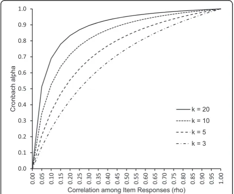
We assume that there are k items in an instrument, i.e., j =1, 2, …, k. The Cα (1) of k items under model (2) and aforementioned assumptions can be expressed as
Cα¼ kσ 2 μ
σ2 eþkσ2μ
¼ kρ
1þρðk−1Þ: ð6Þ
It is due to the fact thatΣ¼σ2
eIþσ2μ11T under model (2) whereIis ak-by-kidentity matrix.Cαin equation (6)
is seen to be an increasing function of both ρ and kas depicted in Fig. 1. Therefore, the number of items needs to be fixed for comparison of Cα of several candidate
sets of items. It follows that for a fixed number of items, higherCαis associated with smaller measurement error of
items through higher inter-item correlationρ. From equa-tion (6),ρcan be expressed in terms ofCαas follows:
ρ¼ Cα
k−Cαðk−1Þ: ð7Þ
Of note, the corresponding correlation matrix is de-noted byΡ¼ð1−ρÞIþρ11T, an equi-correlation matrix.
Thekcorrelated items are often summed up to a scale that is intended to measure the target construct. The scale score is denoted here by
Si¼Xk j¼1
Yij;
which can be viewed as an observed summary score for the i-th subject. Suppressing the subscription i inSi, its mean and variance can be obtained as follows:
Ejð Þ ¼S kμi; ð8Þ
and
V ar Sð Þ ¼kσ2f1þρðk−1Þg: ð9Þ
With respect to the mean (8), average scale score Si/k when used as observed score is an unbiased estimate of true scoreμifor thei-th subject. The reliability, denoted here by R, defined as the squared correlation between true score and observed score can be obtained as follows:
Fig. 1Relationship between Cronbach alpha (Cα) and inter-item
R¼Corr2 Si=k;μ i
ð Þ ¼ kρ
1þρðk−1Þ¼Cα: ð10Þ
This equation supports Theorem 3.1 of Novick and Lewis [9] thatR=Cα if and only if the items are parallel.
Since statistical analysis results do not depend on whether
Si/korSiis used, we use the sumSin what follows. With respect the total variance (9), if the total vari-ance, instead of the true score varivari-ance, is assumed to be fixed,Var(S) is an increasing function of ρ, which con-forms to an elementary statistical theory that variance of sum of correlated variables increases with increasing correlation. On the contrary, under the fixed true score variance assumption, it can be seen that Var(S) is a decreasing function of ρ since equation (9) can be re-expressed in terms ofσ2
μvia equation (5) as follows:
Var Sð Þ ¼kσ2
μð1=ρþk−1Þ ¼k2σ2μ=Cα: ð11Þ
The last equation is due to equation (7). It follows that
Var(S) is also a decreasing function of Cα. In sum, in-crease ofρ decreases the magnitude ofσ2which in turn decreases the magnitude ofVar(S); therefore such indir-ect decreasing effindir-ect ofρ onVar(S) is larger than direct increasing effect ofρonVar(S) in equation (9).
Cronbach alpha and test-retest correlation
Reliability R of instruments is sometimes evaluated by test-retest correlation [3]. Based on model (2), the test and retest item scores can be specified as Yijtest¼μiþeij and Yijretest¼μiþeij, respectively with a common μifor both test and retest scores for each subject,i= 1, 2,…,N. The test-retest correlation can then be measured by the correlation, denoted by Corr(Stest, Sretest), between scale
scoresStest¼
Xk
j¼1Y
test
ij andSretest¼
Xk
j¼1Y
retest
ij repre-senting the scale scores of test and retest, respectively. Under the aforementioned assumptions for model (2) it can be shown that
Cov Sð test; SretestÞ ¼k2ρσ2; ð12Þ
and from equation (10)
V ar Sð testÞ ¼V ar Sð retestÞ ¼kσ2f1þρðk−1Þg: ð13Þ
It follows that:
Corr Sð test; ;SretestÞ ¼ Cov Stest;Sretest
ð Þ
ffiffiffiffiffiffiffiffiffiffiffiffiffiffiffiffiffiffiffiffi Var Sð testÞ
p ffiffiffiffiffiffiffiffiffiffiffiffiffiffiffiffiffiffiffiffi Var Sð testÞ
p
¼ kρ
1þρðk−1Þ¼R¼Cα: ð14Þ
This equation shows that the test-rest correlation is the same as both Cα and R due to equations (6) and
(10), which provides another interpretation of Cα. This
property is especially useful when there is only one item available, in which case estimation of Cα or ρ is
impos-sible by definition. However, the test and retest scores can be thought of as two correlated parallel item scores, and thus their correlation can serve as Cα of the single
item. It is particularly fitting since ρ=Cα=R based on
either equation (6), (7), or (14) whenk= 1.
Taken together, the power φCα of testing significance ofCαagainst any null value should be equivalent to that
of testing significance of a correlation using a Fisher’s z-transformation as long as items are parallel, that is,
φCα¼1−Φ Φ
−1ð1−α=2Þ−pffiffiffiffiffiffiffiffiffiN−3 1 2ln
1þCα 1−Cα
þ Cα 2ðN−1Þ
for a two-tailed significance level α, where Φis the cu-mulative distribution function of a standardized normal distribution, and Φ−1 is its inverse function, i.e.,
Φ(Φ−1(x)) =Φ−1(Φ(x)) =x. We note that although it is necessary to be added for validation of unbiasedness of the test statistics under the null hypothesis, the probabil-ity under the other rejection area will be ignored for all test statistics considered herein. For general covariance structures for non-parallel items, however, many other tests for significance of reliability and Cα have been de-veloped [10–17].
Pre-post comparison
We consider application of a paired t-test to the case of comparison of within-group means of scale scores between pre- and post-interventions. Based on model (2), the pre- and post-intervention item scores can be specified as Yijpre¼μiþeij and Yijpost¼μiþδPPþeij, respectively; the mean of the post-intervention item scores are shifted by δPP, an intervention effect. Con-sequently, we have
E Spost
−E Spre
¼kδpp; ð15Þ
where Spre¼ Xk
j¼1Y pre
ij and Spost¼ Xk
j¼1Y post
ij are the pre- and post-intervention scale scores, respectively. A moment estimate ofδPPfrom (15) can be estimated as
^
δPP¼ Spost −Spr e
=k; ð16Þ
where S ¼XNi¼ 1
Xk
j¼1Yij=N and Nis the total number of subject. Its variance can be obtained as
Var δ^PP
¼2 1ð −ρÞσ2
kN ¼
2 1ð =ρ−1Þσ2 μ
kN : ð17Þ
VarSpost−Spre
¼
VarSpostþVarSpre
−2CovSpost; ;Spre
¼kσ2f1þρðk−1Þg=Nþkσ2f1þρðk−1Þg=N−2k2ρσ2=N
¼2kσ2ð1−ρÞ=N¼2kσ2
μð1=ρ−1Þ=N:
The following test statistic can then be used for testing H0:δ= 0
TPP¼
^ δPP
ffiffiffiffiffiffiffiffiffiffiffiffiffiffiffiffiffiffiffiffiffi Var ^δPP
r ¼ ffiffiffiffiffiffi kN p ^ δPP
σμpffiffiffiffiffiffiffiffiffiffiffiffiffiffiffiffiffiffiffi2 1ð =ρ−1Þ ¼
ffiffiffiffi N p
Spost−Spre
σμpffiffiffiffiffiffiffiffiffiffiffiffiffiffiffiffiffiffiffiffiffi2kð1=ρ−1Þ:
ð18Þ
Now, the statistical power φPP of TPP for detecting non-zeroδPPcan be expressed as follows:
φPP¼Φ δ PP=σμ
ffiffiffiffiffiffiffiffiffiffiffiffiffiffiffiffiffiffiffi kN 2 1ð =ρ−1Þ s
−Φ−1ð1−α=2Þ
( )
:
ð19Þ
This statistical power is an increasing function ofρfor a fixedσμ, which we assume. It follows that the power is also an increasing function ofCαas seen next. WhenδPP is standardized by σμ and ρ is replaced by equation (7), equation (19) can further be expressed in terms of ΔPP¼δPP=σμ and Cα as follows:
φPP¼Φ Δj PPj
ffiffiffiffiffiffiffiffiffiffiffiffiffiffiffiffiffiffiffiffiffiffi N 2 1ð =Cα−1Þ s
−Φ−1ð1−α=2Þ
( )
: ð20Þ
This power function is seen to be independent of k, the number of items. Stated differently, the power will be the same between two instruments with different numbers of items as long as theirCα’s are the same even
if the correlation of items will be smaller for the instru-ment with fewer items.
When sample size determination is needed for a study using an instrument of any number of items with a known Cα for a desired statistical power φ, typically
80 %, it can be determined from equation as follows:
N¼2 1ð =Cα−1Þz2α;φ
Δ2 PP
; ð21Þ
where
zα;φ¼Φ−1ð1−α=2Þ þΦ−1ð Þφ: ð22Þ
The sample size (21) is seen to be a decreasing func-tion of increasing Cα and Δ. In a possibly rare case in
which determination of number of items with known correlations among them is needed for development of an instrument, it has to be determined from equation (19), instead of equation (20), as follow:
k¼2 1ð =ρ−1Þz 2 α;φ NΔ2
PP :
ð23Þ
Comparison of within-group effects between groups In clinical trials, it is often of interest to compare within-group changes between within-groups. For instance, a clinical trial can be designed to compare of pre-post effect of an experimental treatment between treatment and control groups, that is, an interaction effect between group and time point. Based on model (2), the pre- and post-intervention item scores can be specified as
Ypreð Þ0
ij ¼μ0
ð Þ
i þeij and Yijpostð Þ0 ¼μ0
ð Þ
i þδ0þeij for the control group Yijpreð Þ1 ¼μð Þi1 þeij and Yijpostð Þ1 ¼μð Þi1
þδ1þeij for the treatment group. The primary inter-est will be tinter-esting Ho: δBW=δ1 – δ0= 0, i.e., whether or not the difference in pre-post differences between groups will be the same. Consequently, we have
E Df trtð ÞS g−E Df controlð ÞS g ¼kδBW; ð24Þ
where Dtrtð Þ¼S Spostð Þ−S1 preð Þ1¼
Xk
j¼1Y
postð Þ1
ij −
Xk
j¼1Y
preð Þ1
ij
and Dcontrolð ÞS can be similarly defined. A moment esti-mate ofδBWfrom (24) can be obtained as
^
δBW¼Dtrt −Dco ntrol=k; ð25Þ
where N is the number of subjects per group, Dtrt ≡Dtrt S
ð Þ ¼ Spost ð Þ1 −Spr eð Þ1 ¼
XN
i¼1 Xk
jY postð Þ1 ij =N−
XN
i¼1 Xk
jY preð Þ1
ij =N, and,Dco ntrol can similarly be defined. The
variance of^δWBis
Var δ^BW
¼4 1ð −ρÞσ2
kN ¼
4 1ð =ρ−1Þσ2μ
kN : ð26Þ
Therefore, the following test statistic can be used for testing the null hypothesis Ho:δBW= 0,
TBW¼
^
δBW ffiffiffiffiffiffiffiffiffiffiffiffiffiffiffiffiffiffiffiffiffiffi
Var ^δBW
r ¼ ffiffiffiffiffiffi kN p ^ δBW 2σμpffiffiffiffiffiffiffiffiffiffiffiffiffiffiffiffiffið1=ρ−1Þ¼
ffiffiffiffi
N
p
Dtrt−Dcontrol
2σμpffiffiffiffiffiffiffiffiffiffiffiffiffiffiffiffiffiffiffikð1=ρ−1Þ :
ð27Þ
The statistical power φBW of TBW for detecting non-zeroδBWcan thus be expressed as follows:
φBW¼Φ δ BW=σμ
ffiffiffiffiffiffiffiffiffiffiffiffiffiffiffiffiffiffiffi kN 4 1ð =ρ−1Þ s
−Φ−1ð1−α=2Þ
( )
:
ð28Þ
further be expressed in terms of ΔBW¼δBW=σμ and Cα
as follows:
φBW¼Φ Δj BWj
ffiffiffiffiffiffiffiffiffiffiffiffiffiffiffiffiffiffiffiffiffiffi N 4 1ð =Cα−1Þ s
−Φ−1ð1−α=2Þ
( )
: ð29Þ
Again, this power function is seen to be independent ofk, the number of items.
Sample size for a desired statistical power φ can be determined from (27) as follows:
N¼4 1ð =Cα−1Þz 2 α;φ
Δ2
BW :
ð30Þ
Again, this sample size (30) is seen to be a decreasing function of increasingCαandΔ. When number of items is needed for development of an instrument, it can be determined from equation (28) as follow:
k¼2 1ð =ρ−1Þz 2 α;φ NΔ2
BW :
ð31Þ
Two-sample between-group comparison
Comparison of means between groups using an in-strument is widely tested in clinical trials. Based on model (2), the intervention item scores from control and treatment groups can be specified as Yð Þij0 ¼μiþeij
and Yð Þij1 ¼μiþδTSþeij, respectively. The primary inter-est will be tinter-esting Ho: δTS= 0, i.e., whether or not the means are the same between the two groups. Under this formulation, we have
E Sð trtÞ ¼E Sð controlÞ þkδT S; ð32Þ
where Strt¼Xkj¼ 1Y
1 ð Þ
ij and Scontrol¼ Xk
j¼1Y 0 ð Þ ij repre-sents scale scores under treatment and control groups, respectively. A moment estimate ofδTS can be obtained from (32) as
^
δTS¼ Strt −Sco ntrol
=k; ð33Þ
whereStrt¼
XN
i¼1
Xk
j¼1Y 1
ð Þ
ij =N,Sco ntrol¼
XN
i¼1 Xk
j¼1Y 0 ð Þ ij
=N and Nis the number of participants per group. The variance ofδ^TScan be obtained as
Var δ^TS
¼2 1f þρðk−1Þgσ2 kN ¼2 1f =ρþk−1gσ
2 μ
kN : ð34Þ
The corresponding test statisticTTScan be built as
TTS¼
^
δTS ffiffiffiffiffiffiffiffiffiffiffiffiffiffiffiffiffiffiffiffiffi
Var δ^TS
r ¼
ffiffiffiffiffiffi
kN
p
^
δTS σμpffiffiffiffiffiffiffiffiffiffiffiffiffiffiffiffiffiffiffiffiffiffiffiffiffiffiffi2 1ð =ρþk−1Þ
¼ ffiffiffiffi
N
p
Strt−Scontrol
σμpffiffiffiffiffiffiffiffiffiffiffiffiffiffiffiffiffiffiffiffiffiffiffiffiffiffiffiffiffiffi2kð1=ρþk−1Þ:
ð35Þ
And the power functionφTSofTTScan be expressed as
φTS¼Φ δ TS=σμ
ffiffiffiffiffiffiffiffiffiffiffiffiffiffiffiffiffiffiffiffiffiffiffiffiffiffiffi kN 2 1ð =ρþk−1Þ s
−Φ−1ð1−α=2Þ
( )
:
ð36Þ
It should be noted that this statistical power (36) is also an increasing function ofρin contrast to a situation when a fixed total variance assumption is more reason-able in which bothσ2
e and σ2μ are a function ofρbut σ2 is not. For example, observations without measurement errors from clusters are often assumed to be correlated and power of between-group tests using such correlated observations is a decreasing function of ρ [18]. Again, when δTS is standardized by σμ and ρ is replaced by equation (7), equation (33) can further be expressed in terms can further be expressed in terms of ΔTS¼δTS= σμandCαas follows:
φTS¼Φ Δj TSj
ffiffiffiffiffiffiffiffiffiffiffiffiffiffi CαN=2 p
−Φ−1ð1−α=2Þ
n o
: ð37Þ
Again, this power function is seen to be independent ofk, the number of items.
Sample size for a desired statistical power φ can be determined from (37) as follows:
N¼ 2z 2 α;φ CαΔ2BW
: ð38Þ
Again, the sample size (38) is seen to be a decreasing function of increasingCαandΔ. When number of items is needed for development of an instrument, it can be determined from equation (36) as follow:
k¼2 1ð =ρ−1Þz2α;φ=Δ 2 TS N−2z2
α;φ=Δ2TS
: ð39Þ
Results
We fix a two-tailed significance level of α= 0.05 and σ2
μ= 1 without loss generality for all simulations, and de-termineσ2
e andσ 2
throughρdetermined by given kand
Cα. We randomly generate 1000 data sets for each
com-bination of design parameters that include effect size Δ, number of items k, and sample size N. We then com-pute empirical power φ~ by counting data sets from which two-tailed p-values are smaller than 0.05; that is,
~
φ¼X1000s 1ðps<αÞ=1000 where ps represents a two-sided p-value from the s-th simulated data set. For the testing, we applied corresponding t-tests assuming the variances of the moment estimates are unknown, which is practically reasonable. We used SAS v9.3 for the simulations.
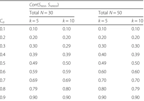
Test-retest correlation
The results are presented in Table 1 that shows the em-pirically estimated test-retest correlations (i.e., average of 1000 estimated Pearson correlations for each set of de-sign parameter specifications) are approximately the same as the pre-assignedCα, regardless of sample sizeN,
which is as small as 30, and number of items k. There-fore, equality betweenCαand test-retest correlation (14)
is well validated.
Pre-post intervention comparison
Table 2 shows that the theoretical powerφPP(20) is very close to the empirical power φ~PP obtained through the simulations. The results validate that the power φPP in-creases with increasingCα(or equivalently increasing
cor-relation for the same k) in the “pre-post” test settings, regardless of sample size Nand number of items k. Fur-thermore, it shows that the statistical power does not depend onkfor a givenCαeven if correlationρdoes.
Between-group whithin-group comparison
Table 3 shows that the theoretical powerφBW(29) is very close to the empirical power φ~BW obtained through the simulations. Therefore, the results validate that the statis-tical power φBW increases with increasing Cα for testing
hypotheses concerning between-group effects on within-group changes regardless ofN, sample size per group, and
k. Again, it shows that the statistical power does not depend onkfor a givenCαeven if correlationρdoes.
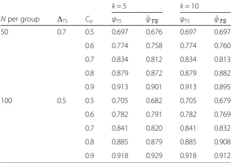
Two-sample between-group comparison
Table 4 shows again that the theoretical powerφTS(37) is very close to the empirical power φ~TS obtained through the simulations. The results validate that the statistical power increases with increasing Cronbachαeven for two-sample testing in cross-sectional settings that does not
Table 1Empirical simulation-based estimates of test-retest correlationCorr(Stest,Sretest) in equation (14)
Corr(Stest,Sretest)
TotalN= 30 TotalN= 50
Cα k= 5 k= 10 k= 5 k= 10
0.1 0.10 0.10 0.10 0.10
0.2 0.20 0.20 0.20 0.20
0.3 0.30 0.29 0.30 0.30
0.4 0.39 0.39 0.40 0.39
0.5 0.49 0.50 0.49 0.50
0.6 0.59 0.59 0.60 0.60
0.7 0.69 0.69 0.70 0.70
0.8 0.79 0.80 0.80 0.79
0.9 0.90 0.90 0.90 0.90
Note: TotalN: total number of subjects;Cα: Cronbach alpha;k: number of items
Table 2Statistical power of the pre-post testTPP(18):σμ= 1
k= 5 k= 10
TotalN ΔPP Cα φPP ~φPP φPP φ~PP
30 0.4 0.5 0.341 0.337 0.341 0.310
0.6 0.475 0.459 0.475 0.458
0.7 0.658 0.626 0.658 0.649
0.8 0.873 0.849 0.873 0.830
0.9 0.996 0.997 0.996 0.995
50 0.3 0.5 0.323 0.309 0.323 0.296
0.6 0.451 0.424 0.451 0.433
0.7 0.630 0.633 0.630 0.614
0.8 0.851 0.849 0.851 0.844
0.9 0.994 0.995 0.994 0.992
Note: TotalN: total number of subjects;k: number of items;ΔPP¼δPP=σμ;Cα:
Cronbach alpha;φPP: theoretical power (20);φ~PP: simulation-based empirical power
Table 3Statistical power of the between-group within-group testTBW(25):σμ= 1
k= 5 k= 10
Nper group ΔBW Cα φBW φ~BW φBW φ~BW 30 0.4 0.5 0.194 0.179 0.183 0.194
0.6 0.268 0.264 0.254 0.268
0.7 0.387 0.375 0.359 0.387
0.8 0.591 0.618 0.594 0.591
0.9 0.908 0.884 0.901 0.908
50 0.3 0.5 0.164 0.184 0.214 0.184
0.6 0.242 0.254 0.261 0.254
0.7 0.387 0.367 0.365 0.367
0.8 0.511 0.564 0.591 0.564
0.9 0.893 0.889 0.893 0.889
Note:Nper group: number of subjects per group;k: number of items;
ΔBW¼δBW=σμ;Cα: Cronbach alpha;φBW: theoretical power (27);φ~BW:
involve within-group effects. it shows that the statistical power does not depend on k for a given Cα even if correlation ρ does. Again, it shows that the statistical power does not depend on k for a given Cα even if correlation ρ does.
Discussion
We demonstrate by deriving explicit power functions that higher internal consistency or reliability of unidimensional parallel instrument items measured by Cronbach alphaCα
results in greater statistical power of several tests regardless of whether comparisons are made within or between groups. In addition, the test-retest reliability correlation of such items is shown to be the same as Cronbach alphaCα.
Due to this property, testing significance of Cα can be
equivalent to testing that of a correlation through the Fisher z-transformation. Furthermore, all of the power functions derived herein can even be applied to trials using single item instrument with measurement error since the power function depends only on Cα which can be estimated via
test-retest correlations for single item instruments as men-tioned earlier. The demonstrations are made theoretically, and validations are made through simulation studies that show that the derived test statistics and their corresponding power functions are very close to each other. Therefore, the sample size determination formulas (21), (30), and (38) are valid and so are the determinations of number of items (22), (31), and (39) in different settings.
In fact, for longitudinal studies aiming to compare within-group effects using such as TPP (18) and TBW (27), the fixed true score variance assumption is not crit-ical since the true score μi’s in model (2) are cancelled by taking differences ofYbetween pre and post-interventions and thus makes the variance of the pre-post differences
depend only on measurement error variance σ2e. For ex-ample, the variance equations (17) and (26) can be expressed in term of only σ2
e, a decreasing function of ρ,
through equation (4) as follows: Var δ^PP
¼2σ2
e=ðkNÞ
and Var ^δBW
¼4σ2
e=ðkNÞ. In other words, both the
power functionsφPP(20) andφBW(29) are increasing func-tion ofCαorρregardless of whether total variance or true
score variance is assumed fixed.
In contrast, however, for cross-sectional studies aiming to compare between-group effects using TTS (35), the fixed true score variance assumption is crit-ical since the variance equation (34) cannot be expressed only in term of only σ2e, and furthermore it can be shown that under a fixed total variance
as-sumption Var δ^TS
(34) is an increasing function of ρ (see equation (10)) and so is the power function. In sum, the fixed true score variance assumption en-ables all of the power functions to be an increasing function of Cα or ρ in a unified fashion. For
ex-ample, Leon et al. [20] used a real data set of HRSD ratings to empirically demonstrate that the statistical power of a two-sample between-group test is in-creasing with increased Cα, although they increased Cα by increasing number of items k, not necessarily
by increasing ρ for a fixed number of items.
In most cases, item scores are designed to be binary or ordinal scores on a likert scale. Therefore, the applicability of the derived power functions and sample size formulas to such cases could be in question since the scores are not normally distributed. Furthermore, it is not easy to build a model like (2) for non-normal scores particularly because measurement error variances depend on the true construct value. For example, variance of a binary score is a function of its mean. Perhaps, construction of marginal models in the sense of generalized estimating equations [21] can be considered for derivation of power functions assumption even if this approach is beyond the scope of the present study. After all, we believe that our study results should be able to be applied to non-normal scores by virtue of the central limit theorem. Another prominent limitation of our study is the very strong assumption of essen-tially τ-equivalent parallel items which may not be realistic at all [8], albeit conceivable for a unidimensional construct. Therefore, further development of power func-tions under relaxed condifunc-tions reflecting more real world situations should be a valuable future study.
Conclusion
Instruments with greater Cronbach alpha should be used for any type of research since they have smaller meas-urement error and thus have greater statistical power for Table 4Statistical power of the between-group within-group
testTTS(32):σμ= 1
k= 5 k= 10
Nper group ΔTS Cα φTS φ~TS φTS φ~TS 50 0.7 0.5 0.697 0.676 0.697 0.697
0.6 0.774 0.758 0.774 0.760
0.7 0.834 0.812 0.834 0.813
0.8 0.879 0.872 0.879 0.882
0.9 0.913 0.901 0.913 0.895
100 0.5 0.5 0.705 0.682 0.705 0.679
0.6 0.782 0.791 0.782 0.769
0.7 0.841 0.820 0.841 0.832
0.8 0.885 0.879 0.885 0.908
0.9 0.918 0.929 0.918 0.912
Note:Nper group: number of subjects per group;k: number of items;
ΔTS¼δTS=σμ;Cα: Cronbach alpha;φTS: theoretical power (34);φ~TS:
any research settings, cross-sectional or longitudinal. However, when items are parallel targeting a unidimen-sional construct, Cronbach alpha of an instrument should be enhanced by developing a set of highly corre-lated items but not by unduly increasing the number of items with inadequate inter-item correlations.
Abbreviations
HRSD:Hamilton Rating Scale of Depression.
Competing interests
The authors declare that they have no competing interest.
Authors’contributions
MH developed the methods, conducted simulation studies, and prepared a draft. NK and MSF provided critical reviews, corrections and revisions. All authors read and approved the final version of the manuscript.
Authors’information
MH is a PhD in Statistics and Professor of Epidemiology and Population Health with collaborative backgrounds in Psychiatry. NK holds dual PhD’s in Statistics and is Assistant Research Professor of Radiology. MSF is a PhD in Psychology and Associate Professor of Nutrition.
Availability of data and materials
Not applicable.
Acknowledgements
We are grateful to the late Dr. Andrew C. Leon for initial discussion of the problems under study.
Funding
This work was in part supported by the NIH grants P30MH068638, UL1 TR001073, and the Albert Einstein College of Medicine funds.
Author details
1
Department of Epidemiology and Population Health, Albert Einstein College of Medicine, 1300 Morris Park Avenue, Bronx, NY 10461, USA.2Department of
Radiology, Albert Einstein College of Medicine, 1300 Morris Park Avenue, Bronx, NY 10461, USA.3Department of Nutrition, Gillings School of Public
Health, University of North Carolina—Chapel Hill, Chapel Hill, NC 27599, USA.
Received: 18 April 2015 Accepted: 18 September 2015
References
1. Hamilton M. A rating scale for depression. J Neurol Neurosurg Psychiatry. 1960;23:56–62.
2. Nunnally JC, Bernstein IH. Psychometric Theory. 3rd ed. New York: McGraw-Hill; 1994.
3. Lord FM, Novick MR. Statistical Theories of Mental Test Scores. Reading, MA: Addison-Wesley; 1968.
4. Schmitt N. Uses and abuses of coefficient alpha. Psychol Assess. 1996;8(4):350–3.
5. Cronbach L. Coefficeint alpha and the internal struture of tests. Psychometrika. 1951;16:297–334.
6. Bland JM, Altman DG. Cronbach’s alpha. Br Med J. 1997;314(7080):572–2. 7. Cortina JM. What is coefficient alpha - An exmination of theory and
applications. J Appl Psychol. 1993;78(1):98–104.
8. Sijtsma K. On the Use, the Misuse, and the Very Limited Usefulness of Cronbach’s Alpha. Psychometrika. 2009;74(1):107–20.
9. Novick MR, Lewis C. Coefficient alpha and the reliability of composite measurements. Psychometrika. 1967;32(1):1–13.
10. Charter RA. Statistical approaches to achieving sufficiently high test score reliabilities for research purposes. J Gen Psychol. 2008;135(3):241–51. 11. Feldt LS, Charter RA. Estimating the reliability of a test split into two parts of
equal or unequal length. Psychol Methods. 2003;8(1):102–9.
12. Feldt LS, Ankenmann RD. Determining sample size for a test of the equality of alpha coefficients when the number of part-tests is small. Psychol Methods. 1999;4(4):366–77.
13. Feldt LS, Ankenmann RD. Appropriate sample size for comparing alpha reliabilities. Appl Psychol Meas. 1998;22(2):170–8.
14. Padilla MA, Divers J, Newton M. Coefficient Alpha Bootstrap Confidence Interval Under Nonnormality. Appl Psychol Meas. 2012;36(5):331–48. 15. Bonett DG, Wright TA. Cronbach’s alpha reliability: Interval estimation,
hypothesis testing, and sample size planning. J Organ Behav. 2015;36(1):3–15. 16. Bonett DG. Sample size requirements for testing and estimating coefficient
alpha. J Educ Behav Stat. 2002;27(4):335–40.
17. Bonett DG. Sample size requirements for comparing two alpha coefficients. Appl Psychol Meas. 2003;27(1):72–4.
18. Donner A, Birkett N, Buck C. Randomization by cluster. Sample size requirements and analysis. Am J Epidemiol. 1981;114(6):906–14. 19. Goldstein H. Multilevel Statistical Models. 2nd ed. New York: Wiley & Sons;
1996.
20. Leon AC, Marzuk PM, Portera L. More reliable outcome measures can reduce sample size requirements. Arch Gen Psychiatry. 1995;52(10):867–71. 21. Zeger SL, Liang KY, Albert PS. Models for longitudinal data - A generalized
estimating equation approach. Biometrics. 1988;44(4):1049–60.
Submit your next manuscript to BioMed Central and take full advantage of:
• Convenient online submission
• Thorough peer review
• No space constraints or color figure charges
• Immediate publication on acceptance
• Inclusion in PubMed, CAS, Scopus and Google Scholar
• Research which is freely available for redistribution