Jacksonet al. BMC Medical Research Methodology2012,12:157 http://www.biomedcentral.com/1471-2288/12/157
R E S E A R C H A R T I C L E
Open Access
An exploration of the missing data mechanism
in an Internet based smoking cessation trial
Dan Jackson
1*, Dan Mason
2, Ian R White
1and Stephen Sutton
2Abstract
Background: Missing outcome data are very common in smoking cessation trials. It is often assumed that all such missing data are from participants who have been unsuccessful in giving up smoking (“missing=smoking”). Here we use data from a recent Internet based smoking cessation trial in order to investigate which of a set of a priori chosen baseline variables are predictive of missingness, and the evidence for and against the “missing=smoking” assumption. Methods: We use a selection model, which models the probability that the outcome is observed given the outcome and other variables. The selection model includes a parameter for which zero indicates that the data are Missing at Random (MAR) and large values indicate “missing=smoking”. We examine the evidence for the predictive power of baseline variables in the context of a sensitivity analysis. We use data on the number and type of attempts made to obtain outcome data in order to estimate the association between smoking status and the missing data indicator. Results: We apply our methods to the iQuit smoking cessation trial data. From the sensitivity analysis, we obtain strong evidence that older participants are more likely to provide outcome data. The model for the number and type of attempts to obtain outcome data confirms that age is a good predictor of missing data. There is weak evidence from this model that participants who have successfully given up smoking are more likely to provide outcome data but this evidence does not support the “missing=smoking” assumption. The probability that participants with missing outcome data are not smoking at the end of the trial is estimated to be between 0.14 and 0.19.
Conclusions: Those conducting smoking cessation trials, and wishing to perform an analysis that assumes the data are MAR, should collect and incorporate baseline variables into their models that are thought to be good predictors of missing data in order to make this assumption more plausible. However they should also consider the possibility of Missing Not at Random (MNAR) models that make or allow for less extreme assumptions than “missing=smoking”.
Background
Missing outcome data are a very common problem in smoking cessation trials. It is common that any such miss-ing data are assumed to correspond to smokers [1-4]. This assumption could be justified by the notion that anyone in a trial who successfully gives up smoking will report this fact. Foulds et al. [5] provide some evidence that missing data are smokers. Hajek and West [6] argue that the “missing=smoking” assumption is plausible because “successful quitters are usually keen to let the treatment providers know of their success” and that “treatment fail-ures feel embarrassed”. The Russell standard requires that
*Correspondence: [email protected] 1MRC Biostatistics Unit, Cambridge, UK
Full list of author information is available at the end of the article
smokers lost to follow-up are classified as continuing to smoke [6,7].
However the evidence from Foulds et al. is of limited value because it is based upon just fifty participants with missing outcome data. Furthermore this was in a hospital setting and there is no reason why this should translate to other settings, and in particular to an Internet based trial. Although some may find the “missing=smoking” assump-tion plausible, and this provides a simple way to handle the missing data, it is open to immediate criticism. One reason for this is because imputing missing outcome data as smokers is a single imputation based procedure, which does not take into account the uncertainty in the missing values [8, p. 45]; if the “missing=smoking” assumption is incorrect then measures of uncertainty, such as standard errors, can be artificially and very considerably dimin-ished. “Missing=smoking” also assumes that all quitters
respond. Finally, the “missing=smoking” assumption tac-itly assumes that any baseline and intermediate data have no additional value for predicting the outcome for partic-ipants whose outcome is unknown.
A further source of concern is the bias in the esti-mated treatment effect that may result from incorrectly assuming “missing=smoking”. Nelsonet al.[9] show that this assumption is “as likely to lead to liberal estimates as to conservative estimates relative to the complete case analysis” and argue that better statistical methods are needed for handling missing data in the tobacco cessa-tion research community. Barneset al.[10] investigate a range of methods for handling missing data in their trial and conclude that imputing missing data as smokers “can cause a large amount of bias if imputing smoking is an incorrect assumption”.
The principal contribution of this paper is the use of empirical evidence to explore the plausibility of different missing data models in the context of a smoking cessa-tion trial. Our aim is to determine which variables play an important role in these models. Particular interest lies in the role of the outcome itself, in order to assess the appropriateness of the “missing=smoking” assumption.
The rest of this paper is set out as follows. We begin by introducing the iQuit trial, an Internet based smoking cessation trial with a large amount of missing outcome data [11]. Here we also describe ten baseline covari-ates that were thought, a priori, to be potential predic-tors in the missing data model. We also describe the repeated attempts that were made by the trial investiga-tors to obtain outcome data. In section “Which baseline variables are predictive of missingness? A selection model approach”, we develop our selection model, where we assess whether any of the baseline variables play an impor-tant role in the missing data model, whilst also allowing the outcome itself to influence this in a sensitivity analy-sis. The attempt to simultaneously estimate the baseline covariate and the outcome effects in this selection mod-elling framework was, as anticipated, not very successful so in section “Is the primary trial outcome predictive of missingness? Modelling the repeated attempts” we describe and use our model for the repeated attempts made to obtain outcome data. Finally we summarise our findings and draw conclusions for smoking cessation tri-alists.
The iQuit trial
The iQuit trial is an Internet based smoking cessation ran-domised controlled trial to assess the benefit of self-help smoking cessation materials tailored to individual smoker characteristics over generic self-help materials, conducted among the general population of smokers seeking help from web-based sources [11]. Participants sign up for the trial via the QUIT website (www.quit.org.uk). They fill
in a questionnaire and receive an online advice report to help them quit smoking. They are randomised either to receive the tailored version or the generic version. Six months later they receive a telephone interview to find out whether they are still smoking, see if their smoking-related beliefs have changed at all, and find out what they thought of the advice they received.
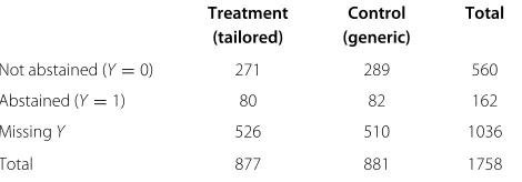
The primary iQuit trial outcome is whether or not participants have abstained from smoking (self-reported three months prolonged abstinence) and the primary research question is whether or not tailored materials are more effective than generic materials in helping par-ticipants achieving this. The corresponding analysis is described in detail by Mason et al. [11], who found a lack of evidence for a treatment effect. However, and despite the intensive follow up from the trialists to obtain outcome data, there is a large amount of missing data; smoking status is unknown for 1036 of the 1758 par-ticipants (59%). This compromises the primary analysis, as explained by Mason et al., but provides an excellent opportunity to investigate the reasons for missing data. The pattern of missing data is summarised in Table 1.
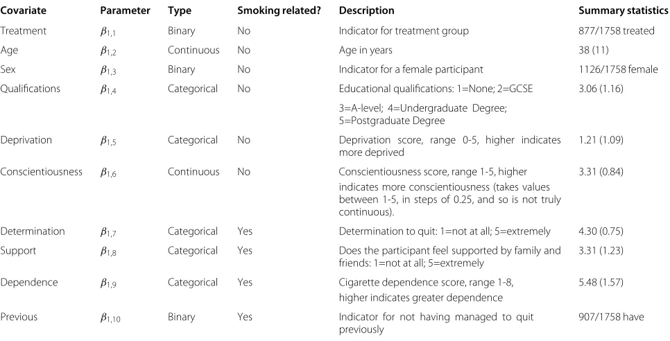
In addition to the primary trial outcome, a wide range of complete (no missing data) baseline variables were mea-sured, and those thought a priori to be most likely to be good predictors of missing data are summarised in Table 2. Some of the variables in Table 2 are referred to as ‘smoking related’ variables because they are consid-ered to more directly relate to the participant’s smoking behaviour. An aim here is to investigate which, if any, of these variables are good predictors, whilst allowing for the possibility that the primary trial outcome itself may also be predictive of its missingness.
The iQuit trial provides the rich data on the number and type of attempts made to obtain outcome data shown in Table 3. It was specified in the trial design that partic-ipants would receive up to ten telephone calls to obtain outcome data and, for those of whom all calls were unsuc-cessful, where possible a single further attempt was made by email. The telephone attempts ceased when outcome data was obtained, the number given by the participant was found to be invalid or the participant requested that no further telephone calls were made. The decision to
Table 1 The pattern of missingness for the primary trial
outcomeY
Treatment Control Total (tailored) (generic)
Not abstained (Y=0) 271 289 560
Abstained (Y=1) 80 82 162
MissingY 526 510 1036
Jacksonet al. BMC Medical Research Methodology2012,12:157 Page 3 of 12 http://www.biomedcentral.com/1471-2288/12/157
Table 2 Baseline covariates
Covariate Parameter Type Smoking related? Description Summary statistics
Treatment β1,1 Binary No Indicator for treatment group 877/1758 treated
Age β1,2 Continuous No Age in years 38 (11)
Sex β1,3 Binary No Indicator for a female participant 1126/1758 female
Qualifications β1,4 Categorical No Educational qualifications: 1=None; 2=GCSE 3.06 (1.16)
3=A-level; 4=Undergraduate Degree; 5=Postgraduate Degree
Deprivation β1,5 Categorical No Deprivation score, range 0-5, higher indicates
more deprived
1.21 (1.09)
Conscientiousness β1,6 Continuous No Conscientiousness score, range 1-5, higher 3.31 (0.84) indicates more conscientiousness (takes values
between 1-5, in steps of 0.25, and so is not truly continuous).
Determination β1,7 Categorical Yes Determination to quit: 1=not at all; 5=extremely 4.30 (0.75)
Support β1,8 Categorical Yes Does the participant feel supported by family and
friends: 1=not at all; 5=extremely
3.31 (1.23)
Dependence β1,9 Categorical Yes Cigarette dependence score, range 1-8, 5.48 (1.57)
higher indicates greater dependence
Previous β1,10 Binary Yes Indicator for not having managed to quit
previously
907/1758 have
Summary statistics are shown where means and standard deviations (in parentheses) are given for the continuous and categorical variables.
make telephone calls to obtain outcome data was made in order to ensure good quality data and so that the medium of follow-up was not the same as the medium of inter-vention. Multiple telephone calls were made in order to facilitate calling participants at different times of the day but no more than ten calls were made to avoid harassing them. The email was a ‘last ditch’ effort to obtain outcome data where the telephone calls had failed. These repeated attempts to obtain data provide the basis for our mod-elling in section “Is the primary trial outcome predictive of missingness? Modelling the repeated attempts”.
Which baseline variables are predictive of missingness? A selection model approach
Here a selection modelling approach [8, p. 30] is used in order to investigate the missing data model in smoking cessation trials. The modelling allows for an association between the trial outcome and the missing data indica-tor but also accommodates less extreme assumptions than “missing=smoking”. We extend this approach in the next section by using data on the repeated attempts to obtain outcome data [12-15].
For the sake of generality, for the moment we use vec-tors to denote the outcomes but in our application these quantities are scalars. LetYi denote theith participant’s vector of outcomes, so that participants may provide more than a single outcome, and letRidenote the correspond-ing vector of misscorrespond-ing data indicators, whereRi,j = 1 if
Yi,jis observed, whereYi,jandRi,jare thejth entries ofYi
andRirespectively. We letxidenote theith participant’s covariates and we posit a model forYi|xi. We then posit a model Ri|(Yi,xi), which is referred to as the selection model. We model the joint distribution of(Yi,Ri)|xiusing the factorisation provided by these two models.
A common assumption is that the data are Missing at Random (MAR). The data are said to be MAR, given the covariatesxiif, for alli,Riis independent of the missing entries ofYi, given those that are observed andxi. Equiv-alently, the MAR assumption can be expressed as the requirement that the density of Ri|(Yi,xi) depends only onYithrough the entries that are observed. However it is not clear from this definition whether MAR requires this condition for the observed pattern of missing data or for all possible patterns of missing data under repeated sam-pling. The definition of MAR of Lu and Copas [16] makes this requirement explicit for all possible missingness pat-terns and they show that, with the further assumption that separate parameters are used in the models for the out-come and the selection model, their definition of MAR implies that the model for the missing dataRi|(Yi,xi)is ignorable and valid inferences for the outcome param-eters can be made using just the outcome model and the observed outcome data. A caveat however is that the observed, rather than the expected, information matrix should be used to obtain standard errors [17].
Table 3 The outcomeYby the number of contact attempts and trial arm
Attempts Participants Responded Of responders % quit
One phone call 217 214 50/214=23.4%
One phone call and an email
925 69 30/69 =43.5%
Two phone calls 134 132 23/132=17.4%
Two phone calls and an email
6 1 0/1=0%
Three phone calls 93 89 16/89=18.0%
Three phone calls and an email
3 0 0/0
Four phone calls 59 57 10/57=17.5%
Four phone calls and an email
4 0 0/0
Five phone calls 48 45 9/45=20.0%
Five phone calls and an email
8 0 0/0
Six phone calls 19 19 1/19=5.3%
Six phone calls and an email
2 1 1/1=100%
Seven phone calls 38 38 5/38=13.2%
Seven phone calls and an email
2 0 0/0
Eight phone calls 17 16 3/16=18.8%
Eight phone calls and an email
5 1 1/1=100%
Nine phone calls 11 10 2/10=20%
Nine phone calls and an email
2 0 0/0
Ten phone calls 19 19 6/19=31.6%
Ten phone calls and an email
146 11 5/11=45.5%
The fraction and percentage of participants who successfully quit smoking (Y=1) are tabulated by the number of contact attempts (telephone calls and email). Participants received up to ten telephone calls and up to one email attempt.
indicator is permitted. Although the model for the out-come is usually of central interest, because this contains population parameters such as a treatment effect, here the focus of interest lies in the selection model. This is because this model describeswhydata are missing, and so we also refer to this model as the missing data model.
We are primarily interested in determining which vari-ables play an important role in this model. One reason why this investigation is important is because MAR analy-ses are made more plausible by including variables that are good predictors of missingness: if they predict missing-ness sufficiently well so that any role of missingYiis non-existent, or at least negligible, then the MAR assumption is adequate. It is however important to know what kind
of additional variables smoking cessation trialists should routinely collect and incorporate into models to make MAR more plausible. These variables may be modelled as covariates if we are prepared to adjust for them [18], or as further response variables if we are not [18,19]. Another reason why this investigation is important is to determine whether or not the outcome itself is a useful predictor of missingness, in order to assess whether MNAR mod-elling is required. However, since every MNAR model has a MAR counterpart with equal fit [20], it is only by mak-ing distributional assumptions, such as those that follow, that this type of assessment can be made.
We will defineYi=1 if theith participant has abstained from smoking andYi = 0 otherwise andRias the corre-sponding missing data indicator. We definexi as theith participant’s row vector of ten covariates, in the order they appear in Tables 2 and 4. SinceYiandRiare both binary, we use conventional logistic regression modelling for both variables and we assume that
logit(P(Yi =1|xi))=α0+α1xi (1)
and
logit(P(Ri =1|Yi=yi,xi))=β0+β1xi+β2yi. (2)
IfRi = 0 thenYiis missing and is ‘summed out’ of the log-likelihood in (3) below. Hence participants who do not provide outcome data contribute to the analysis. We fur-ther assume that participants are independent. The first α1parameter, which we denote as α1,1 is the (adjusted)
treatment effect, but here the focus of interest is on the covariates that are important in the missing data model, ie β1 and β2 are paramount. The parameter β2 is the
adjusted log odds ratio betweenYi andRi. This param-eter is therefore of particular interest because a positive infiniteβ2 is equivalent to assuming “missing=smoking”.
Ifβ2 = 0 then the data are MAR, otherwise the data are
MNAR. We address the difficulty in estimatingβ2later.
Separate parameters are used for the outcome (α parame-ters) and the selection model (theβparameters) so MAR implies that the missing data model is ignorable [16]. In this case the models (1) and (2) can be fitted as two sepa-rate conventional logistic regressions, where model (1) is fitted using the complete cases.
A participant for whomYi is observed (Ri = 1) con-tributes P(Yi = yi|xi)P(Ri = 1|Yi = yi,xi) to the likelihood, and a participant for whomYiis not observed providesP(Ri = 0|xi) =
Ja
ck
so
n
et
a
l.
B
MC
Medica
lR
esea
rch
Meth
o
d
o
lo
g
y
2012,
12
:157
Page
5
o
f
1
2
http://www.biome
dce
n
tral.com/1471-2288/12/157
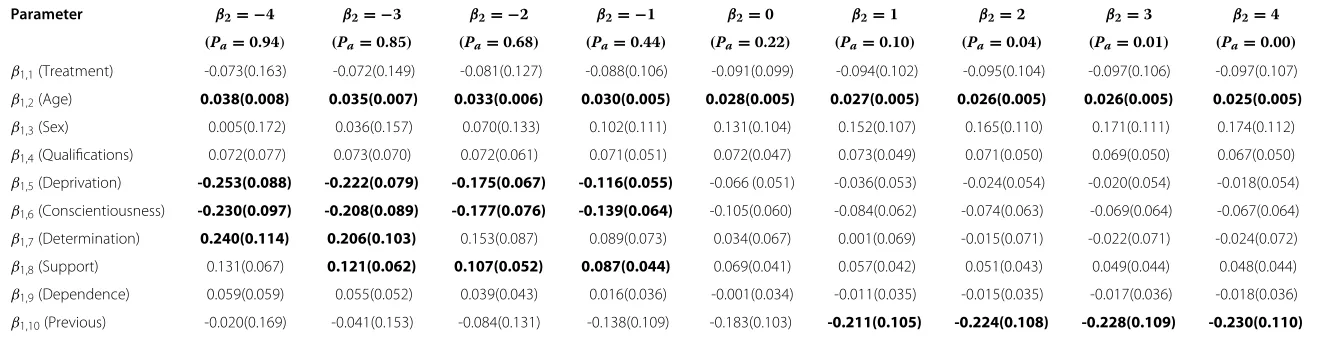
Table 4 The results from the sensitivity analysis
Parameter β2= −4 β2= −3 β2= −2 β2= −1 β2=0 β2=1 β2=2 β2=3 β2=4
(Pa=0.94) (Pa=0.85) (Pa=0.68) (Pa=0.44) (Pa=0.22) (Pa=0.10) (Pa=0.04) (Pa=0.01) (Pa=0.00) β1,1(Treatment) -0.073(0.163) -0.072(0.149) -0.081(0.127) -0.088(0.106) -0.091(0.099) -0.094(0.102) -0.095(0.104) -0.097(0.106) -0.097(0.107)
β1,2(Age) 0.038(0.008) 0.035(0.007) 0.033(0.006) 0.030(0.005) 0.028(0.005) 0.027(0.005) 0.026(0.005) 0.026(0.005) 0.025(0.005)
β1,3(Sex) 0.005(0.172) 0.036(0.157) 0.070(0.133) 0.102(0.111) 0.131(0.104) 0.152(0.107) 0.165(0.110) 0.171(0.111) 0.174(0.112)
β1,4(Qualifications) 0.072(0.077) 0.073(0.070) 0.072(0.061) 0.071(0.051) 0.072(0.047) 0.073(0.049) 0.071(0.050) 0.069(0.050) 0.067(0.050)
β1,5(Deprivation) -0.253(0.088) -0.222(0.079) -0.175(0.067) -0.116(0.055) -0.066 (0.051) -0.036(0.053) -0.024(0.054) -0.020(0.054) -0.018(0.054)
β1,6(Conscientiousness) -0.230(0.097) -0.208(0.089) -0.177(0.076) -0.139(0.064) -0.105(0.060) -0.084(0.062) -0.074(0.063) -0.069(0.064) -0.067(0.064)
β1,7(Determination) 0.240(0.114) 0.206(0.103) 0.153(0.087) 0.089(0.073) 0.034(0.067) 0.001(0.069) -0.015(0.071) -0.022(0.071) -0.024(0.072)
β1,8(Support) 0.131(0.067) 0.121(0.062) 0.107(0.052) 0.087(0.044) 0.069(0.041) 0.057(0.042) 0.051(0.043) 0.049(0.044) 0.048(0.044)
β1,9(Dependence) 0.059(0.059) 0.055(0.052) 0.039(0.043) 0.016(0.036) -0.001(0.034) -0.011(0.035) -0.015(0.035) -0.017(0.036) -0.018(0.036)
β1,10(Previous) -0.020(0.169) -0.041(0.153) -0.084(0.131) -0.138(0.109) -0.183(0.103) -0.211(0.105) -0.224(0.108) -0.228(0.109) -0.230(0.110)
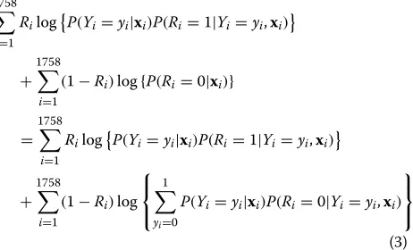
yi,xi). The log-likelihood of the data provided by all 1758 participants isL(α0,α1,β0,β1,β2)=
1758
i=1
RilogP(Yi=yi|xi)P(Ri=1|Yi=yi,xi)
+ 1758
i=1
(1−Ri)log{P(Ri=0|xi)}
= 1758
i=1
RilogP(Yi=yi|xi)P(Ri=1|Yi=yi,xi)
+ 1758
i=1
(1−Ri)log ⎧ ⎨ ⎩ 1
yi=0
P(Yi=yi|xi)P(Ri=0|Yi=yi,xi) ⎫ ⎬ ⎭ (3)
where the probabilities necessary to compute this likeli-hood are evaluated in terms of theα andβ parameters from equations (1) and (2). Participants who provide out-come data (Ri = 1) contribute to the first summation in (3) and those who do not provide outcome data (Ri = 0) contribute to the second summation.
Modelling the covariates
Complete case logistic regressions (analyses that assume MAR) were performed for the outcomes Y on each of the categorical variables in Table 2 in turn, where the regressions treated these variables as categorical and then continuous. Deviance tests (comparing the fitted logistic regressions treating these variables as categorical and con-tinuous), suggested that treating the categorical variables as continuous in the model (1) is adequate. Similar results were obtained for regressions of the missing data indica-tor, providing reassurance that treating these variables as continuous in (2) is also adequate.
In situations where the treatment of categorical vari-ables as continuous does not appear so reasonable, two approaches might be considered. First the categorical vari-ables could be treated as such, but the additional dummy variables will make the already computationally demand-ing nature of MNAR modelldemand-ing yet more so. An alternative is to dichotomise categorical variables, where care is taken to ensure that there is a reasonable amount of data in both groups and, ideally, the sensitivity of the results to the decisions made when dichotomising variables is assessed. A limitation of our investigations of the treatment of the categorical variables as continuous is that these are from standard logistic regressions, which assume data are MAR, but the computationally intensive nature of using the full likelihood very much reduced the appeal of using MNAR models in preliminary investigations of this kind.
We also investigated the possibility that quadratic terms for the two continuous covariates in Table 2 might be required in (1) and (2); no evidence was found that these
are required to describe the data. More sophisticated transformations of continuous covariates, for example using spline functions or fractional polynomials, could also be considered but these would add to the computa-tional demands and were not explored. As a final point, interactions between the ten covariates could be con-sidered. The introduction of further parameters to the likelihood also adds to the computational demands and this was not investigated, in part because of this, but also because we merely wish to assess which covariates present themselves as important predictors in model (2), for which our modelling is adequate.
A sensitivity analysis
The estimation of the full selection model using the log-likelihood (3) is generally discouraged because the model fit is so fragile; it is highly dependent on distributional assumptions and is sensitive to outlying or unusual obser-vations [21]. Sensitivity analyses are therefore generally encouraged and so we adopt this approach in this section, where β2 is used as the sensitivity parameter. We know
thatβ2 = 0 (MAR) generally provides a stable model fit
so we anticipate that this will also be so for alternative fixed values of β2. However this can only assess
base-line covariate effects assuming particular values for the sensitivity parameter, and cannot quantify the evidence that the outcome itself is important in the missing data model. We return to the estimation of the full selection model in section “Fitting the full model’’. For the moment we are content to address the question of which baseline variables play an important role in the missing data model. In our sensitivity analysis, we constrainβ2, to nine
val-ues: -4, -3, -2, -1, 0 , 1, 2, 3, 4. The valuesβ2were chosen
because they cover a wide range of possibilities. This can be seen by noting that
β2=logit(P(Ri=1|Yi=1,xi))−logit(P(Ri=1|Yi=0,xi)) which, because the odds ratio treats the two variables being compared symmetrically, is equivalent to
β2= −(logit(P(Yi=1|Ri=0,xi))
−logit(P(Yi =1|Ri=1,xi)))= −log(IMOR) (4)
where ‘IMOR’ is the Informatively Missing Odds Ratio of Higginset al [22]. We take the covariatesxi as referring to a typical participant who hasP(Y =1|R= 1,x)equal to the observed abstention rate in the complete cases, ie P(Y = 1|R = 1,x) = 162/722 ≈ 0.22. We can then approximately convertβ2values toP(Yi = 1|Ri = 0,xi),
using equation (4). This approximate conversion from β2 to P(Y = 1|R = 0,x) gives the values shown in
Table 4, where we see that β2 = −4 corresponds to a
Jacksonet al. BMC Medical Research Methodology2012,12:157 Page 7 of 12 http://www.biomedcentral.com/1471-2288/12/157
to less than a 0.5% abstention rate which is tantamount to assuming “missing=smoking”. Hence the sensitivity analy-sis explores a very wide range of possibilities.
As explained above, the MAR model (β2 = 0) can
eas-ily be fitted as separate logistic regressions. The remaining eight models are fitted by numerically maximising the log-likelihood (3), where parameter estimates’ standard errors are obtained from the observed information matrix, which is also obtained numerically. The log-likelihood was coded in R and themaxLikpackage was used to obtain the maxi-mum likelihood estimates and their standard errors in this way. Starting values are required by themaxLikcommand and the MAR fit was used as starting values forβ2= −1
andβ2=1, and the resulting estimates were used as
start-ing values forβ2= −2 andβ2=2, and so on. Despite this,
several hours of computing time was needed to fit each of the eight models. The iQuit data are not freely available but indicative R code is available from the first author on request.
From Table 4 we have very robust inferences that age is an important predictor in the missing data model; no matter what value we assume for β2 we obtain strong
evidence that older participants are more likely to pro-vide outcome data. Epro-vidence, at the 5% level, that the nonsmoking related variables ‘deprivation’ and ‘conscien-tiousness’ are important predictors requires negativeβ2,
which means that participants with missing data are more likely to have given up smoking than those who provide outcome data. Those who consider “missing=smoking” plausible are unlikely to entertain negativeβ2but such
val-ues might be justified by assuming that participants who have given up smoking are more likely to lose contact with the trial, because they no longer need its support, and so are in fact less likely to provide outcome data. Even if this possibility were entertained, it is clear that the significance of all non-smoking related covariate effects, other than the effect of age, are sensitive toβ2 and hence the assumed
role of the outcome in the selection model.
From Table 4, the significance of the smoking related covariates are also sensitive to the assumed value ofβ2;
although some analyses provide significant effects, no covariate effect can be found at the 5% level that is not sensitive to the assumedβ2. Only by making strong
assumptions about the value ofβ2can covariate effects be
inferred.
To summarise the conclusions from the sensitivity anal-ysis, the only baseline covariate that appears to be safely regarded as important in the missing data model is the age of participants. However other variables may also be important, depending on range ofβ2thought plausible.
Fitting the full model
Despite our reservations about the full MNAR model fit being so fragile, we also fitted this model by numerically
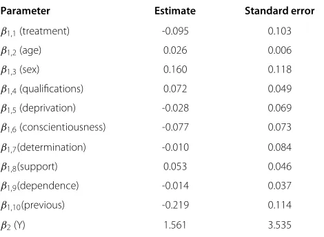
maximising the log-likelihood (3). This was achieved by using the MAR model fit as the starting point for the numerical maximisation and the resulting estimated miss-ing data model is shown in Table 5. This model is (very weakly) identified by the assumptions made in the lin-ear predictor in model (2). A saturated logistic regression model for the situation where data were available for all four combinations of outcome and missing data indicator is not identifiable here, because we do not observe data where the missing data indicator is 0. Hence the model identification must come from the form of model (2), which assumes linearity and no interactions.
A comparison of the MARβ1estimates in Table 4 with
the corresponding MNAR estimates in Table 5 suggests these are not very sensitive to the choice between assum-ing MAR or allowassum-ing this form of MNAR. The effect of age is again strongly significant, providing further weight to the evidence that this plays an important role in the miss-ing data model. The standard errors of theβ1parameters
increase slightly when allowing MNAR, but not as much as might be anticipated from the uncertainty in the esti-mate ofβ2in Table 5; a 95% confidence interval for this
parameter is (-5.4, 8.5) which includes all of the possibil-ities considered in the sensitivity analysis. Again making use of (4), the lower and upper bounds of the 95% con-fidence interval for β2 are close to “missing=cessation”
and “missing=smoking” respectively so it it not possible to make any statement about the plausibility, or otherwise, of the commonly made ‘missing=smoking” assumption from this analysis. In any case, even if the standard error ofβ2
had been much smaller, any conclusions about the role of the outcome would be open to criticism due to issues surrounding the fitting of MNAR models [21].
Table 5 Estimates from the full selection model
Parameter Estimate Standard error
β1,1(treatment) -0.095 0.103
β1,2(age) 0.026 0.006
β1,3(sex) 0.160 0.118
β1,4(qualifications) 0.072 0.049
β1,5(deprivation) -0.028 0.069
β1,6(conscientiousness) -0.077 0.073
β1,7(determination) -0.010 0.084
β1,8(support) 0.053 0.046
β1,9(dependence) -0.014 0.037
β1,10(previous) -0.219 0.114
β2(Y) 1.561 3.535
Is the primary trial outcome predictive of missingness? Modelling the repeated attempts In order to overcome the problems associated with the estimation of MNAR missing data models using selec-tion models, models for the repeated attempts to obtain outcome data have been proposed [12-15]. This type of modelling is possible where a number of attempts to obtain outcome data are made, as is the case for the iQuit trial: as explained above, participants in the iQuit trial receive between one and ten telephone calls to obtain outcome data, and if these are unsuccessful they receive where possible a further attempt by email. Participants may receive less than ten telephone calls and then an email if, for example, they request that no more telephone calls are made and do not provide data, or if the tele-phone number they have provided is found to be invalid. The assumption that underlies the modelling is that out-come data from participants who require many attempts to obtain are more like those with missing data than those who require fewer attempts.
We now model the probability that a particular attempt at obtaining outcome data is successful, rather than the marginal probability that outcome data is obtained as in selection modelling. We continue to assume model (1) and we replace model (2) with our model for the attempts to obtain outcome data
logit(P(Ri,m=1|Yi=yi,xi)=β0,m+β1xi+β2yi (5) where Ri,m is equal to one if the mth attempt, m = 1, 2· · ·11, to obtain outcome data from theiparticipant is successful; the email attempt is modelled as the 11th attempt regardless of the number of telephone calls made. We allow the email attempt to be more or less success-ful than the telephone attempts via its interceptβ0,11 but
make the simplification that the probability of obtaining outcome data in this way does not depend on the num-ber of telephone calls that preceded it. This is reasonable because the email is a very different way to obtain out-come data and and this represents a pragmatic approach to modelling because the email was not very successful (only 83 participants provided data in response to over a thousand emails). This assumption is relaxed as part of the sensitivity analysis below. Model (5) can be thought of as a discrete survival model, or a stratified logistic regression, where we also handle the unobserved outcomes.
Each attempt has its own intercept β0,m, so that, for
example, earlier attempts may be more successful than later ones but the identifying assumption is that the covariate effects are common across attempts. The appro-priateness of this assumption for the baseline covariates was assessed by including an attempt by covariate inter-action in the MAR model. Two of these interinter-actions were statistically significant at the 5% level (age, p-value=0.04;
qualifications, p-value=0.01). On a closer examination the apparent interaction between attempt and qualifications is largely explained by the observation that more educated participants appear to be more likely to respond to the email. Adding an interaction between the email attempt alone and the baseline covariates resulted in only one sta-tistically significant interaction at the 5% level: the test for the presence of a qualifications by email interaction pro-vided a p-value of 0.0004, where the log odds ratio asso-ciated with a unit increase in educational qualifications is 0.38. This may be plausible, because more educated par-ticipants could have greater access to, and command of, computing facilities. However, since a very small propor-tion of email attempts were successful, this finding should be cautiously interpreted. Despite this, more sophisticated modelling of the missing data model could commence by allowing this interaction.
Now that model (5) has replaced model (2), we refer to model (5) as the missing data model. If a single attempt is made to obtain outcome data from all participants then model (5) simplifies to (2), hence the model for the repeated attempts is an extension of the selection model.
The numbers and percentages of participants who suc-cessfully give up smoking (Yi = 1) are shown by the number and type of attempts to obtain outcome data in Table 3. Finding patterns in the results for those who do not respond the telephone calls and hence are sent an email is difficult, because such little outcome data is obtained in this way, but the data for those who respond to a telephone call is slightly suggestive of a decreas-ing probability of smokdecreas-ing cessation as the number of attempts increases: fitting a complete case logistic regres-sion of smoking cessation on the number of attempts for these participants gives an estimated slope of -0.03 (with a standard error of 0.04). Although not significant, the fitted model predicts that the probability of smoking ces-sation decreases with the number of attempts. Therefore we anticipate a positive estimated association betweenYi andRi,mwhen fitting model (5), so that those who have
given up smoking are more likely to provide outcome data than those who have not.
The proportion of those giving up smoking is higher in those who respond to the email rather than a telephone call in Table 3. This could be because this method for obtaining outcome data, although less likely to obtain data per se, is relatively more likely to obtain outcome data from nonsmokers than smokers. If true this would inval-idate the assumption that theβ2 coefficient is the same
for the email as the telephone attempts. Since estimating a separateβ2for the email attempt would encounter the
same type of estimation problems as in section “Fitting the full model”, an alternative would be to constrain theβ2for
Jacksonet al. BMC Medical Research Methodology2012,12:157 Page 9 of 12 http://www.biomedcentral.com/1471-2288/12/157
The likelihood is similar in form to (3) but, now that each attempt to obtain outcome data contributes to this, its form is more complex and is shown in the Appendix. The MAR model (β2 = 0) was fitted as separate logistic
regressions ofYionxi, andRi,jonxiand attempt number,
in the same manner as for the MAR model in the sensi-tivity analysis above. This MAR model was then used as a starting value for the numerical maximisation of the full log-likelihood and standard errors can be obtained from the observed information matrix as before.
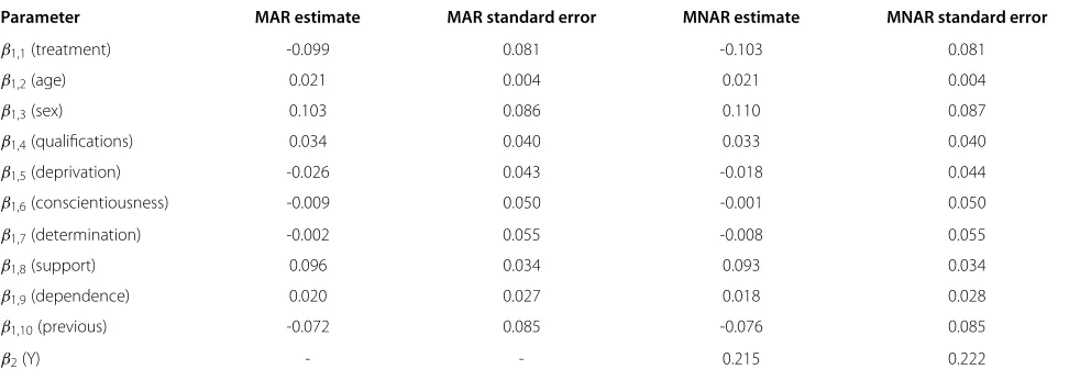
The fitted MAR and MNAR repeated attempts models are shown in Table 6. The estimates of theβ1parameters
are not sensitive to the choice between MAR or MNAR and only slightly larger standard errors for these param-eters are obtained when allowing the data to be MNAR. From Table 6 we see that the participant’s age is confirmed as having an important role in the missing data model and the effect of support (of family and friends) is also statistically significant, where participants who feel more supported are also more likely to provide outcome data. This analysis suggests that both smoking related (support) and non-smoking related (age) variables are good predic-tors of missing data so it would appear that both types of variables may play important roles in the missing data model.
The model for the repeated attempts has enabled us to identify the effect of the trial outcome in the missing data model because the standard error ofβˆ2is acceptably
small. This is in sharp contrast with the results for the cor-responding results using the selection model in section “Fitting the full model”. The estimate of β2 is positive
as expected but the analysis, which rests on the distri-butional assumptions described above, does not rule out the possibility that data are MAR because β2 = 0 lies
within the 95% confidence interval. We next explore what
probabilities are predicted for smoking cessation in the missing data.
A guide to the probability of abstaining from smoking for participants who do not provide outcome data
Let{R}idenote the set ofRi,mobserved for participanti; for example if a participant receives two telephone calls and an email then their{R}i = {Ri,1,Ri,2,Ri,11}. For such a participant with missing data {R}i = {0, 0, 0} = {0}. From Bayes’ Theorem we obtain the odds that participants with missing data are smokers, given the failed attempts to obtain outcome data, as
P(Yi =1|{R}i= {0},xi) P(Yi =0|{R}i= {0},xi) =
P(Y
i=1|xi) P(Yi=0|xi)
×
P({R}i= {0}|Y1=1,xi)
P({R}
i= {0}|Y1=0,xi)
(6)
The terms in the first curly bracket on the right hand side of (6) can be obtained from model (1) and the prob-abilities that each of the Ri,m that are members of{R}i are zero can be obtained from model (5). Hence the odds, and therefore the probability, of not smoking given the failed attempts can be evaluated for participants with missing data. When fitting the full model using maximum likelihood, models (1) and (5) are fitted simultaneously. Using the MNAR maximum likelihood estimates to eval-uate P(Yi = 1|{R}i = {0},xi) for all participants with missing data, and taking the average, gives a marginal probability of participants with missing data being non-smokers of 0.17; 162/722=22% of those with observed outcomes are nonsmokers (Table 1). This analysis suggests that fewer participants with missing data are nonsmokers
Table 6 Estimates from the model for the repeated attempts
Parameter MAR estimate MAR standard error MNAR estimate MNAR standard error
β1,1(treatment) -0.099 0.081 -0.103 0.081
β1,2(age) 0.021 0.004 0.021 0.004
β1,3(sex) 0.103 0.086 0.110 0.087
β1,4(qualifications) 0.034 0.040 0.033 0.040
β1,5(deprivation) -0.026 0.043 -0.018 0.044
β1,6(conscientiousness) -0.009 0.050 -0.001 0.050
β1,7(determination) -0.002 0.055 -0.008 0.055
β1,8(support) 0.096 0.034 0.093 0.034
β1,9(dependence) 0.020 0.027 0.018 0.028
β1,10(previous) -0.072 0.085 -0.076 0.085
β2(Y) - - 0.215 0.222
but does not support the “missing=smoking” assumption. For comparison, using the maximum likelihood estimates but replacingβ2 with a value two standard errors above
and below its estimate provides a marginal probability of participants with missing data being nonsmokers of 0.14 and 0.19 respectively; using β2 = 0 (MAR) in this
way gives a probability of 0.18. These smaller probabili-ties of participants being nonsmokers, than in the sample of participants who provide outcome data, are partly due to them having covariates that are associated with less chance of giving up smoking but this probability also falls asβ2increases. Hence the choice of covariates that are
included in the modelling affects the proportions of non-responders that are ‘imputed’ as smokers by the model.
This more sophisticated method for translating β2
into the probability that non-responders have abstained, which takes into account covariate effects, could also be used in conjunction with the selection model, but the approach adopted there is considerably simpler and more transparent.
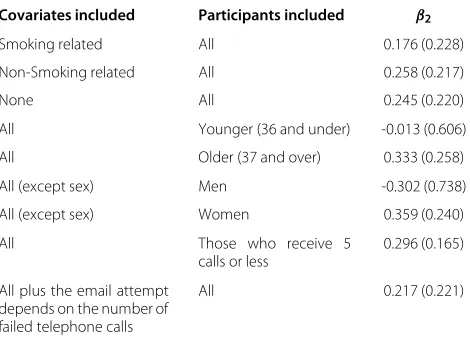
Further sensitivity and subgroup analyses
Since the assertion that the data do not support the “miss-ing=smoking” assumption is such an important conclu-sion, we performed sensitivity analyses in order to assess how robust this inference is. First, we refitted the model including only the smoking related covariates (Table 2), then only the nonsmoking related covariates and then omitting all covariates.
Next we performed our subgroup analyses by fitting the full model to participants of median age (36) or under, and then to the older participants. We then fitted the full model to men and women separately, but omit-ting the now unidentifiable effect of sex. Also, because there are very few participants who receive more than 5 contact attempts, and these participants provide consid-erable weight in the repeated attempts model and might be unusual and influential, an analysis was performed omitting these participants.
Finally the number of telephone calls received was added as a covariate in (5) whenm= 11. This allows the probability of the success of the email attempt to depend on the number of failed telephone calls.
In total this resulted in nine further fitted models and the estimates ofβ2are shown in Table 7. Most of the
esti-mates are similar in sign, magnitude and standard error. The two that differ in sign to the rest (from the analy-ses restricted to male and younger participants) are less well identified. This is reasonable because there are fewer male participants and younger participants are less likely to provide outcome data. Furthermore, these negative point estimates point in the opposite direction to “miss-ing=smoking” and the impression from Table 7 is that none of the models fitted support this assumption.
Table 7 Further estimates ofβ2from repeated attempts modelling
Covariates included Participants included β2
Smoking related All 0.176 (0.228)
Non-Smoking related All 0.258 (0.217)
None All 0.245 (0.220)
All Younger (36 and under) -0.013 (0.606)
All Older (37 and over) 0.333 (0.258)
All (except sex) Men -0.302 (0.738)
All (except sex) Women 0.359 (0.240)
All Those who receive 5
calls or less
0.296 (0.165)
All plus the email attempt depends on the number of failed telephone calls
All 0.217 (0.221)
Estimates ofβ2are shown, with standard errors in parentheses, when omitting particular combinations of covariates and participants.
Conclusions
We have developed two statistical models and have explored the missing data model using the empirical evi-dence from the iQuit trial. In particular we found strong evidence that the participant’s age is a good predictor in this. The evidence that the trial outcome itself is important in this model is much weaker. This casts very considerable doubt on the “missing=smoking” assump-tion. This conclusion is also evident from an inspection of Table 3; one can imagine what would happen if the attempts to obtain outcome data were ceased after fewer attempts. Some nonsmokers in Table 3 would then be lost to follow up and designated as smokers in error by the “missing=smoking” assumption. Future methodolog-ical research could focus on methods for assessing the goodness of fit and other diagnostics for the repeated attempts model.
Perhaps our most important finding is that we estimate the probability not smoking in those failing to provide out-come data to be between 0.14 and 0.19. This excludes both the “missing=smoking” assumption and the MAR analysis that makes makes no use of the baseline covariates (22% of participants who provide outcome data abstained from smoking). This finding, in conjunction with the arguments of Nelsonet al.[9] and Barneset al.[10], provide a case for “missing=smoking” analyses to be abandoned alto-gether. However the MAR assumption seems to be a good option, provided that suitable covariates are collected and included in the model.
Jacksonet al. BMC Medical Research Methodology2012,12:157 Page 11 of 12 http://www.biomedcentral.com/1471-2288/12/157
outcome model using maximum likelihood, in conjunc-tion with either (2) or (5), all parameter estimates are obtained simultaneously. Hence parameter estimates of model (1) could be also presented such as the treat-ment effect, which is usually the parameter of primary interest.
The suspicion that participants with more educational qualifications may be more likely to respond to an email reminds us that the variables that are important in the missing data model are likely to be context specific, and can be anticipated to depend on the nature of the trial and how data are collected. For example, if email was the pri-mary method for obtaining response data then, if correct, this suspicion suggests that qualifications would be a cru-cially important variable to consider when modelling the missing data. Trialists therefore should not take our inves-tigation as a definitive statement of which variables are important in smoking cessation trials in full generality, but our results suggest that both smoking and non-smoking related variables can play a role in this. We therefore recommend that, if additional variables are to be incorpo-rated into the analysis to make the MAR assumption more plausible, trialists should consider both kinds of variables, and also any other variables that they think may explain why their data are missing. A rich set of baseline, and possibly auxiliary post randomisation, variables should be collected for this purpose.
Even if the many such variables are collected and incorporated in the analysis then the possibility that the outcome itself may play a role persists, as epito-mised by the “missing=smoking” assumption. However this requires MNAR modelling and the approaches used here, although suitable for our special investigations, are perhaps too computationally intensive for more routine use. We are therefore developing a simpler MNAR mod-elling approach, where “missing=smoking”, MAR and Last Observation Carried Forward analyses (LOCF [8, p. 45]) are embedded into a much wider class of models. Hence the implications of many possibilities for the treatment effect can be quickly and easily assessed. Despite the computational power that is now available, the trade-off between sophisticated methodology and computa-tionally straightforward methods remains, so we hope that this will make MNAR modelling more accessible to applied researchers and that they will be inspired to attempt this.
Appendix
We continue to let Ri = 1 denote that the ith partici-pant provides outcome data and we let the binary variable Eidenote whether or not an attempt by email was made, whereEi =1 if this was made andEi =0 otherwise. We lettiequal the number oftelephonecall attempts to obtain
outcome data. The log-likelihood of the data is given by L(α0,α1,β0,β1,β2)=
1758
i=1 EiRilog
⎧ ⎨
⎩P(Yi=yi|xi)P(R
i,11=1|Yi=yi,xi)
× ti
j=1
P(Ri,j=0|Yi=yi,xi) ⎫ ⎬ ⎭+ 1758 i=1
(1−Ei)Rilog ⎧ ⎨
⎩P(Yi=yi|xi)P(R
i,ti =1|Yi=yi,xi)
× ti−1
j=1
P(Ri,j=0|Yi=yi,xi) ⎫ ⎬ ⎭+ 1758 i=1
Ei(1−Ri)log ⎧ ⎨ ⎩ 1
yi=0
P(Yi=yi|xi)P(Ri,11=0|Yi=yi,xi)
× ti
j=1
P(Ri,j=0|Yi=yi,xi) ⎫ ⎬ ⎭+ 1758 i=1
(1−Ei)(1−Ri)log ⎧ ⎨ ⎩
1
yi=0
P(Yi=yi|xi)
× ti
j=1
P(Ri,j=0|Yi=yi,xi) ⎫ ⎬ ⎭
where the probabilities necessary to compute this likeli-hood are evaluated in terms of theα andβ parameters from equations (1) and (5). Empty products in this likeli-hood are defined to be one.
Competing interests
The authors declare that they have no competing interest.
Authors’ contributions
DJ performed the statistical analyses and all authors contributed to the writing of the paper. All authors read and approved the final manuscript.
Acknowledgements
The iQuit trial was supported by funding from Cancer Research UK reference no. C4496/A7775. The investigators on the iQuit grant were Ruth Bosworth, Stephen Sutton and Hazel Gilbert.. The authors also wish to acknowledge the work of the staff at QUIT in helping to set up and administer the website, and the contribution of the telephone interviewers. DJ and IRW are employed by the UK Medical Research Council [Unit Programme number U105260558].
Author details
1MRC Biostatistics Unit, Cambridge, UK.2Behavioural Science Group, Institute
of Public Health, University of Cambridge, Cambridge, UK.
Received: 3 April 2012 Accepted: 15 August 2012 Published: 15 October 2012
References
2. Chan SS, Leung DY, Abdullah AS, Wong VT, Hedley AJ, Lam TH:A randomised controlled trial of a smoking reduction plus nicotine replacement therapy intervention for smokers not willing to quit smoking.Addiction2011,106:1153-1163.
3. Smolkowski K, Danaher BG, Seeley JR, Kosty DB, Severson HH:Modeling missing binary outcome data in a successful web-based smokeless tobacco cessation program.Addiction2010,105:1005–1015. 4. Bolliger CT, Zellweger JP, Danielsson T, et al.:Smoking reduction with
oral nicotine inhalers: double blind, randomised clinical trial of efficacy and safety.Br Med J2000,321:329–333.
5. Foulds J, Stapleton J, Hayworth M, et al.:Transdermal nicotine patches with low-intensity support to aid smoking cessation in outpatients in a general hospital.Arch Family Med1993,4:417–423.
6. Hajek P, West R:Commentary on Smolkowski et al (2010): why is it important to assume that non-responders in tobacco cessatoin trials have relapsed?Addiction2010,105:1016–1017.
7. West R, Hajek P, Stead L, Staplton J:Outcome criteria in smoking cessation trials: the need for a common standard.Addiction2005, 100:299–303.
8. Molenberghs G, Kenward MG:Missing data in clinical studies. Chichester UK: Wiley; 2007.
9. Nelson DB, Partin MR, Fu SS, Joseph AM, An LC:Why assigning ongoing tabacco use is not necessarily a conservative approach to handling missing tobacco cessataion outcomes.Nitotine and Tobacco Res2009, 11:77–83.
10. Barnes SA, Larsen MD, Schroeder D, Hason A, Decker PA:Missing data assumptions and methods in a smoking cessation study.Addiction 2010,1105:431–437.
11. Mason D, Gilbert H, Sutton S:Effectiveness of web-based tailored smoking cessation advice reports (iQuit): a randomised trial. Addiction2012 (to appear, doi:10.1111/j.1360-0443.2012.03972.x). 12. Alho JM:Adjusting for non-response bias using logistic regression.
Biometrika1990,77:617–624.
13. Wood AM, White IR, Hotoph, M:Using number of failed contact attempts to adjust for non-ignorable non-response.J R Stat Soc, Ser A 2006,169:525–542.
14. Jackson D, White IR, Leese M:How much can we learn about missing data? An exploration of a clinical trial in psychiatry.J R Stat Soc, Ser A 2010,173:593–612.
15. Akacha M, Hutton JL:Modellng the rate if change in a longitudinal study with missing data, adjusting for contact attempts.Stat Med 2011,30:1072–1089.
16. Lu G, Copas, JB:Missing at random, likelihood ignorability and model completeness.Ann Stat2004,32:754–765.
17. Kenward M, Molenberghs G:Likelihood based frequentist inference when data are missing at random.Stat Sci1998,13:236–247. 18. Carpenter J, Kenward MG:Missing data in randomised clinical trials. Report,
London School of Hygiene and Tropical Medicine; 2008.
19. Ibrahim JG, Lipsitz SR, Horton MG:Using auxillary data for parameter estimation with non-ignorably missing outcomes.Appl Stat2001, 50:361–373.
20. Molenberghs G, Beunckens C, Sotto C, Kenward MG:Every missingness not at random model has a missingness at random counterpart with equal fit.J R Stat Soc, Ser B2008,70:371–388.
21. Kenward MG:Selection models for repeated measurements with non-random dropout: an illustration of sensitivity.Stat Med1998, 17:2723–2732.
22. Higgins JPT, White IR, Wood, AM:Imputation methods for missing outcome data in meta-analysis of clinical trials.Clin Trials2008, 5:225–239.
doi:10.1186/1471-2288-12-157
Cite this article as:Jacksonet al.:An exploration of the missing data mechanism in an Internet based smoking cessation trial. BMC Medical Research Methodology201212:157.
Submit your next manuscript to BioMed Central and take full advantage of:
• Convenient online submission
• Thorough peer review
• No space constraints or color figure charges
• Immediate publication on acceptance
• Inclusion in PubMed, CAS, Scopus and Google Scholar
• Research which is freely available for redistribution