NUMERICAL SIMULATION OF TURBULENT FLOW IN A RECTANGULAR CHANNEL WITH PERIODICALLY MOUNTED LONGITUDINAL VORTEX GENERATORS

NUMERICAL SIMULATION OF TURBULENT FLOW IN A

RECTANGULAR CHANNEL WITH PERIODICALLY MOUNTED

LONGITUDINAL VORTEX GENERATORS

Pankaj Saha

a

and Gautam Biswas

a,b*

a _{Department of Mechanical Engineering, Indian Institute of Technology, Kanpur, U.P, 208016, India}

b_{Central Mechanical Engineering Research Institute (CSIR) Durgapur, Durgapur, W.B, 713209, India}

A

BSTRACT

Detailed flow structure in turbulent flows through a rectangular channel containing built-in winglet type vortex generators have been analyzed by means of solutions of the full Navier-Stokes equations using a Large-Eddy Simulation (LES) technique. The Reynolds number of investigation is 6000. The geometry of interest consists of a rectangular channel with a built-in winglet pair on the bottom wall with common-flow-down arrangement. The winglet pair induces streamwise longitudinal vortices behind it. The vortices swirl the flow around the axis parallel to the mainstream direction and disrupt the growth of thermal boundary layer entailing enhancement of heat transfer. The influence of the longitudinal vortices persist far downstream of the location of the winglet-pair. Since the structure of the turbulence is strongly affected by the streamline curvature, the flow of interest, despite the simplicity of its geometry, turns out to be extremely complex. Therefore it calls for more accurate calculation of the turbulent quantities. In the present study, flow structures are studied by using time-averaged quantities, such as the iso-contours of velocity components, vortices and turbulent stresses. The simulation shows that the secondary flow is stronger in the regions where the longitudinal vortices are more active. The wake like structures of streamwise velocity occurs due to strong distortion of the boundary layer by vortices. The spanwise distributions of turbulent kinetic energy and Reynolds stress show the evidence of strong secondary flow. The computational results compare well with the experimental data qualitatively.

Keywords: LES, vortex generators, coherent structures.

*_{Corresponding author. Email: [email protected]}

1.

INTRODUCTION

Vortex generators are used for flow control and drag reduction on lifting and control surfaces for aerospace applications. Vortex generators can also be used for heat- transfer enhancement. Such applications have led to extensive studies of the effects of vortices on heat transfer augmentation and delayed separation. The vortex generators also act as turbulence promoters at high Reynolds numbers.

An engineering means of generating such vortices is introducing winglets in the flow. Common shapes of such winglets are delta and rectangle. In practice, array of winglets are fabricated on the heat exchanger walls. The winglets induce streamwise longitudinal vortices behind it. The vortices swirl the flow around the axis parallel to the mainstream direction and disrupt the growth of thermal boundary layer. Disruption of thermal boundary layer brings about enhancement of heat transfer. The influence of the longitudinal vortices persists far downstream of the location of the winglets.

Experimental studies of Edwards and Alker (1974); Russel et al. (1982) and Tiggelbeck et al. (1994) reveal the enhancement of heat transfer due to longitudinal vortices. They compared the effects of different types of vortex generators. Torii and Yanagihara (1989) concluded that the reason of heat transfer is connected with high velocity fluctuation, indicating transition from laminar to turbulent

flow. The experimental investigations on transition and turbulent flow regime were conducted by Fiebig et al. (1991). Pauley and Eaton (1988) investigated effects of delta winglets on turbulent boundary layer.

The present work considers channel flow as the base flow with rectangular winglet pair as the vortex generators. This configuration has application in plate-fin heat exchangers and in many internal cooling devices. The vortex generators can make the flow unsteady and induce early transition to turbulence. Numerical and experimental investigations have been conducted in developing and fully developed channel flow by Fiebig et al. (1986); Biswas and Chattopadhyay (1992). Zhu et al. (1995) and Deb et al. (1995) investigated turbulent flows in a channel with longitudinal vortices using standard

k

−

ε

model.

Since the structure of the turbulence is strongly affected by the streamline curvature, the flow of interest, despite the simplicity of its geometry, turns out to be extremely complex. It is felt that the results can be made more reliable through deployment of more accurate turbulence model. In addition, the flow becomes periodically fully developed at the end of some rows of winglets as clearly shown by Brockmeier et al. (1993).

Frontiers in Heat and Mass Transfer

β

h B

L 2H

e l

p

p y

x z

The purpose of the present work is to carry out numerical investigation of turbulence structures in a rectangular channel with periodically mounted rectangular winglet-pair. The feasibility of the present turbulence model have been justified by computing the turbulence quantities and the effects of vortices have been estimated with respect to characteristics of turbulent channel flows.

2.

STATEMENT OF THE PROBLEM

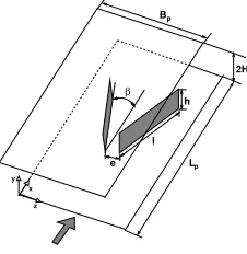
The computations are performed on a three-dimensional periodic channel module with a pair of vortex generators as shown in Fig. 1. The obstacles, in the form of a rectangular winglet pair are attached to the bottom wall of the channel in a common-flow-down arrangement. The flow is considered as incompressible with constant fluid properties. The Reynolds number of interest is 6000. The Reynolds number is defined on the basis of channel half height

( )

H and mean velocity

( )

uav .

Fig. 1Computational domain

2.1

Flow Configuration and Grid System

The computational domain is described in Cartesian coordinate system in which the x-axis is aligned with the streamwise flow direction, the y-axis is in wall normal direction and z-y-axis is in the spanwise direction. The geometrical dimensions are expressed in terms of channel half height H. The relevant dimensions are:

Channel length

( )

L_p : 4πH

Channel width

( )

Bp :

π

H

Channel height : 2H

Angle of attack

( )

β

: 0 15

Winglet length

( )

l

: 4H

Winglet height

( )

h

: H

Spacing between inlet and entry points of winglets:

2 2

p

L l

cosβ

⎛ ⎞

−

⎜ ⎟

⎝ ⎠

The computational domain is divided into a set of rectangular cells. A staggered grid arrangement is used such that the velocity components are defined at the center of cell faces and the pressure is at the center of the cell volume. The number of grid used for this simulation is

66 70 66× × in x, y and z-directions respectively. The uniform grid is adopted in x and z directions. Non-uniform grid distribution based on algebraic stretching function is deployed in the vertical y direction. In the present computation, a fine grid near the wall is used which is sufficient to capture small scales in the viscous sub-layer.

2.2

Governing Equations and Boundary Conditions

The filtered forms of the continuity and the momentum equations for incompressible flows are expressed as follows:

0

i i

u x

∂ ₌

∂

(1)

2 2

( ) 1

Re

i j ij

i i

j i j j

u u

u p u

t x x x x

τ

∂ ∂

∂ _{+ = −}∂ ₊ ∂ ₋

∂ ∂ ∂ ∂ ∂ (2)

where, uis the filtered component of velocity, the index i=1, 2, 3 refers to the x, y and z directions, respectively. The repeated indices imply summation. In the above equations the velocities are non-dimensionalized with the mean flow velocity uav, lengths with channel

half height H and the pressure byρuav2 . The above equations represent

the large scale motion. The effect of small scales appears through a subgrid scale (SGS) stress tensor as:

τij=u ui j−u ui j (3)

Locally dynamic SGS model of Piomelli and Liu (1995) has been used in order to calculate the sub-grid stresses. The detailed procedure is outlined in Srinivas et al. (2006). According to this subgrid-scale model, the SGS stress tensor is expressed as:

1 2 3

i j ij kk TSij

τ − δ τ = −ν (4)

1 2

j i ij

j i

u u

S ( )

x x

∂ ∂

= +

∂ ∂ (5)

where S_ij, represents the resolved rate-of-strain tensor and ν_T is the

eddy viscosity.

The eddy viscosity is formulated as:ν =T

(

CsΔ

)

2S , where

2 _{ij ij}

S = S S is the magnitude of the instantaneous resolved-rate of

strain tensor, Δ is the characteristic smallest length scale retained in the resolved velocity field and Cs is the model coefficient called

Smagorinsky constant. In dynamic model approach, the model constant is computed dynamically as the calculation progresses. In this method, one needs to apply two filters namely grid filter and the test filter. The model coefficients are calculated based on the information of scale contained within the above filter scales. In addition to that, a local averaging of the instantaneous model coefficients is done to avoid ill-conditioning. Once the model-coefficients are obtained, the SGS stress is calculated using the Eq. (4). Periodic boundary conditions are enforced between inlet and outlet and at the side boundaries. The no-slip boundary condition is used at all solid walls including the winglet surfaces.

2.3

Solution Methodology

The solution procedure follows modified version of the Marker and Cell algorithm of Harlow and Welch (1965). In the present study, the spatial discretization uses second-order central differencing for convective and diffusive terms. A second order accurate, Adam-Bashforth scheme is used for time discretization and the pressure term is discretized occasionally by forward differencing. A localized version of dynamic SGS model has been used as a closure. To control the numerical instability that takes place due to negative value of eddy viscosity, the magnitude of the total viscosity ⎡_⎣

(

1 Re

)

+ν_Τ⎤_⎦ is set

y+

U

+

10-1 ₁₀0 ₁₀1 ₁₀2

0 5 10 15 20

DNS ( Moser et al., 1999 ) Present computation

U+_{= y}+

U+_{= (1/k) ln(y}+_{) +C}

U

0 5 10 15 20 25 30 6

8 10

U

0 5 10 15 20 25 30 6

8 10

U

0 5 10 15 20 25 30 6

8 10

U

0 5 10 15 20 25 30 6

8 10

U

0 5 10 15 20 25 30 6

8 10

U

0 5 10 15 20 25 30 6

8 10

Y

U

0 5 10 15 20 25 30 6 8 10 (a) Experimental (b) Numerical Z Y

0.5 1 1.5

0.5 1 1.5 2 0 3 2 -0.0235391 -0.140241 -0.140241 .0727251 0.14469 0.5 1 2 2 1 Z Y

0.5 1 1.5

0.5 1 1.5 2 0 1.0345 0.945752 1.16205 1.0345 1 1.12218 1.15621 1.03 1.1221 1.1415 1 0.945752 1.0345 0.7 0.916165 1.0345 0.916165

1.10 75 18565

Z

Y

0.5 1 1.5

0.5 1 1.5 2

0

(a) (b) (c)

Z

Y

0.5 1 1.5 2 2.5 3

0.5 1 1.5

Z

Y

0.5 1 1.5 2 2.5 3

0.5 1 1.5

Z

Y

0.5 1 1.5 2 2.5 3

0.5 1 1.5

(a) (b) (c)

3.

VALIDATION

The numerical simulation has been first validated for the fully developed turbulent channel flow simulation using DNS data of Moser

et al. (1999), for the same Reynolds number and grid resolution of the

actual problem studied.

Fig. 2Mean streamwise velocity profile (in wall units), Reτ =180

Figure 2 shows the comparison of dimensionless mean velocity

profileU+ as a function of y+. The result agrees well with the DNS data. This ensures that the grid resolution and the LES technique are well capable of capturing the turbulence structure for the present problem and Reynolds number considered. The results have been further compared with the experimental results of Lau (1995). Figure 3 (a) and (b) show the streamwise velocity distributions at an axial distance X = 11, and at different spanwise locations. The numerical results match qualitatively well with its experimental counterpart and both show a wake like profile near to the vortex core. The difference in magnitude occurs due to the fact that the experiment was done at a higher Reynolds number than that of the present simulation.

4.

RESULTS AND DISCUSSION

As mentioned earlier, the flow configuration is common flow down. Initially, the simulation is run without winglet to get a fully developed turbulent flow field in the channel. The results are validated with the available fully developed channel flow data. The simulation is run further with the built-in winglet pair. The time averaged values of the various statistical quantities are determined to understand the complex flow structure.

The computations were allowed to run upto 300 non-dimensional time units with a typical time step size of 0.001 in order to get a stable statistical average. Statistics were accumulated over the last 150 nondimensional time units. From the averaged velocity field, mean flow parameters and flow structures have been determined.

The detailed view of the secondary flow is shown in Fig. 4 (a), (b) and (c). The plot shows secondary velocity vectors, streamwise velocity contours and longitudinal vortices contour at a cross-sectional plane at an axial distance of X = 9 from inlet. The vortex region is identified through the nonvanishing secondary velocity vector. It is seen that the vortex fills the entire cross section of the channel.

Fig. 4 (a) Streamwise velocity contours, (b) Streamwise vorticity

contours, and (c) Velocity vectors (detailed view at X = 9)

The streamwise velocity contours at different axial cross-sectional plane are shown in Fig. 5 (a), (b) and (c). The plots show very thick "mushroom-like" features near the side wall (spanwise). The counter rotation of the vortices lift the low-momentum fluid from the side surfaces in the upward direction, results in thickening of the boundary layer at that section. This zone is called upwash zone. As a result, the high momentum fluids come down in the zone between the vortex generators, create thinning of boundary layer and often called downwash zone. In this case, the direction of flow between the vortices is in downward direction, justifying the nomenclature common-flow down.

Fig. 5 Contours of streamwise velocity at different axial locations:

(a) X = 9, (b) X = 10, and (c) X = 12.

The streamwise vorticity contours (Fig. 6 (a), (b) and (c)) at different axial locations show the spreading of vortices, their interactions and decay of strength along the flow direction.

(b) (c) (a)

U/U_av

Y

0 0.5 1 1.5

0.5 1 1.5 2

upwash vortex core downwash

Reynolds Stress

Y

-0.02 -0.01 0 0.01 0.02

0.5 1 1.5 2

upwash vortex core downwash

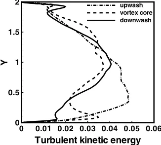
Turbulent kinetic energy

Y

0 0.01 0.02 0.03 0.04 0.05 0.06

0 0.5 1 1.5

2 _upwash

vortex core downwash the distorted features in the vortex core. These features are similar to

that were observed by Liu et al. (1996).

Apart from the mean flow, the other turbulence quantities have been computed. Along this line, the Reynolds shear stress distributions across the channel have been shown in Fig. 8 for different spanwise locations. The features show a strong value in the vortex zone. The turbulent kinetic energy reveals the characteristic features of turbulence. Therefore, this parameter has been computed and plotted in Fig. 9.

Fig. 6 Contours of streamwise vorticity at different axial locations:

(a)X = 9, (b) X = 10, and (c) X = 12

Fig. 7 Mean streamwise velocity profiles at different spanwise

locations (X = 9)

The plots explain the generation of turbulence at different spanwise locations. It is seen that the value shows maximum at the vortex core due to the strong secondary flow. These features have been experimentally captured by Lau (1995) for the similar flow arrangements. It is to be noted that the overlap between the regions of wake-like behavior of streamwise contour and the maximum turbulent kinetic energy is discerned.

Turbulence physics is well explained by using the concepts of vortex dynamics and more specifically, the turbulent shear flow is dominated by spatially coherent vortical motions, known as coherent structure (Moser et al., 1999). According to Chong et al. (1990), the vortex region is identified by the positive second invariant of the deformation tensor. The mathematical formulation is expressed as

Q′ = i j j i

1

u / x . u / x

2 ′ ′

− ∂ ∂ ∂ ∂ 1

(

2 2

)

S 2

= Ω −

,

whereΩand S are the symmetric and antisymmetric components of velocity gradient, u∇ ′. Thus, Q′ establishes a local balance between the strain rate and vorticity magnitude. Therefore, the regions whereQ′ >0, the vorticity is significant and is brought about due to rotation rather than shear.

Fig. 8 Reynolds stress profiles at different spanwise locations (X = 9)

Fig. 9 Turbulent kinetic energy profiles at different spanwise locations

(X = 9)

The iso-surfaces of positive second invariant are shown in Fig. 10. It shows convincing evidence of numerous different vortical structures suggesting existence of vortical arches (hierarchical structures) along with the single streamwise vortices.

5.

CONCLUSIONS

A numerical investigation has been carried out in a fully developed turbulent channel with built-in winglet pair to predict the secondary velocity field by means of large eddy simulation technique. The flows show wake like behavior of the mean streamwise velocity field. Here LES technique with high grid resolution has been deployed to ensure accuracy. The flow field shows good qualitative agreement with the available results. The coherent structures identify the turbulence structures in a rather meaningful sense. The velocity vector and vortices shows strong distortion of the velocity profile and existence of swirling motion. From the flow structures, it can be said that the arrangement is able to enhance heat transfer due to the intensification of mixing. The effects are not only local, but sustain over the long downstream zone. The coefficient of friction due to secondary flow needs a larger pumping power comparable to flows without winglet.

A future work is needed for the possible orientation of the winglet for the maximum heat transfer enhancement and minimum added power overhead.

NOMENCLATURE

Re Reynolds number

t time

u velocity

x coordinate

Greek Symbols

ρ density

Superscripts

0 last time step

Subscripts

0 initial condition

∞ ambient environment

REFERENCES

Biswas, G., and Chattopadhyay, H., 1992, “Heat transfer in a channel with built-in wing-type vortex generators,” Int J Heat Mass Transfer,

35, 803–814.

http://dx.doi.org/10.1016/0017-9310(92)90248-Q

Brockmeier, U., Guentermann, T., and Fiebig, M., 1993, “Performance evaluation of a vortex generator heat transfer surface and comparison with different high performance surfaces,” Int J Heat Mass Transfer,

36, 2575–2587.

http://dx.doi.org/10.1016/S0017-9310(05)80195-4

Chong, M.S., Perry, A.E., and Cantwell, B.J., 1990, “A general classification of three-dimensional flow fields,” Phys Fluid A, 4, 765– 777.

http://dx.doi.org/10.1063/1.857730

Deb, P., Biswas, G., and Mitra, N. K., 1995, "Heat transfer and flow structure in laminar and turbulent flows in a rectangular channel with longitudinal vortices," Int J Heat Mass Transfer, 38, 2427-2444.

http://dx.doi.org/10.1016/0017-9310(94)00357-2

Edwards, F.J., and Alker, C.J., 1974, “The improvement of forced surface heat transfer using Surface protrusions in the form of cubes and vortex generators,” Fifth Int. Heat Transfer Conf., 244-248, Tokey.

Fiebig, M., Kalweit, P., and Mitra, N.K., 1986, “Heat transfer enhancementand Drag by longitudinal vortex generators in a channel flow,” Eighth Int. Heat Transfer Conf., 2909-2914, San Francisco.

Fiebig, M., Kalweit, P., Mitra, N.K., and Tiggelbeck, S., 1991, “Heat transfer enhancement and Drag by longitudinal vortex generators in a channel flow,” Experimental Thermal and Fluid Science, 4, 103–114.

http://dx.doi.org/10.1016/0894-1777(91)90024-L

Harlow, F.H., and Welch, J.E., 1965, “Numerical calculation of time dependent viscous incompressible flow of fluid with free surface,” Phys

Fluid, 8, 2182–2188.

http://dx.doi.org/10.1063/1.1761178

Lau, S., 1995, “Experimental study of the turbulent flow in a channel with periodically arranged longitudinal vortex generators,”

Experimental Thermal and Fluid Science, 11, 255–262.

http://dx.doi.org/10.1016/0894-1777(95)00054-P

Liu, J., Piomelli, U., and Spalart, P.R., 1996, “Interaction between a spatially growing turbulent turbulent layer and embedded streamwise vortices,” Journal of Fluid Mechanics, 326, 151–179.

http://dx.doi.org/10.1017/S0022112096008270

Moser, R.D., Kim, J., and Mansour, N.N., 1999, “Direct numerical simulation of turbulent channel flow up to Re_τ =590,” Phys Fluids, II, 943–945.

http://dx.doi.org/10.1063/1.869966

Pauley, W.R., and Eaton, J.K., 1988, “Experimental Study of the Development of Longitudinal Vortex Pairs Embedded in a Turbulent Boundary Layer,” AIAA J, 26, 816–823.

http://dx.doi.org/10.2514/3.9974

Piomelli, U., and Liu, J., 1995, “Large-Eddy Simulation of Rotating Channel Flows using a Localized Dynamic Model,” Phys Fluid, 7(4), 839–848.

http://dx.doi.org/10.1063/1.868607

Russel, C.M., Jones, T., and Lee, G.H., 1982, “Heat transfer enhancement using vortex generators,” Seventh Int. Heat Transfer

Conf., 283-288, Munich.

Srinivas, Y., Biswas, G., Parihar, A.S., and Ranjan, R., 2006, “Large- Eddy Simulation of High Reynolds Number Turbulent Flow Past a Square Cylinder,” Journal of Engineering Mechanics, 132(3), 327–335.

http://dx.doi.org/10.1061/(ASCE)0733-9399(2006)132:3(327)

Tiggelbeck, S., Mitra, N.K., and Fiebig, M., 1994, “Comparison of wingtype vortex generators for heat transfer enhancement in a channel,”

J Heat Transfer, 116, 880–885.

http://dx.doi.org/10.1115/1.2911462

Torii, K., and Yanagihara, J.I., 1989, “The effects of longitudinal vortices on heat transfer of laminar boundary layer,” JSME Int J Series

II, 32, 359–402.

Zhu, J.X., Fiebig, M., and Mitra, N.K., 1995, “Numerical investigation of turbulent flows and heat transfer in a rib-roughened channel with longitudinal vortex generators,” Int J Heat Mass Transfer, 38, 495–501.