Page | 1
Start up Cost constraint Optimization using
Lagrangian Algorithm for Unit Schedule in
Electrical Power System
Navpreet Singh Tung1, Ashutosh Bhadoria2, Anant Bhardwaj3
1
M.Tech Scholar, Electrical Engg. (Student Member IEEE), Lovely Professional University, India
3
M.Tech Scholar, Electronics and Communication Engg. Lovely Professional University, India
2,
Asst. Professor, Electrical Engg., Lovely Professional University, India
ABSTRACT
Electricity companies typically possess numerous units and they need to commit units because electricity cannot be stored in a large-scale system and demand is a random variable process fluctuating with the time of the day and the day of the week. A problem that must be frequently resolved by a electricity utility is to economically determine a schedule of what units will be used to meet the forecasted demand, and satisfy operating constraints such as start up cost, over a short time horizon. This problem is commonly referred to as the unit commitment (UC)problem. Lagrangian algorithm is one of the technique based on equal IC of fuel input for the units in operation. It is helpful for the optimium load sharing among units, with satisfying constraints under different environment. Simulation algorithm is prepared in this paper, keeping start up cost constraint optimization and simulation is done with Matlab for standard set of Units. Optimized IC and load sharing values are extracted sharing different start up cost. Different IC values are extracted for different load demands.
Keywords: Unit Commitment (UC); Economic Dispatch (ED), Lagrangian Multiplier (LM), Incremental cost (IC), Load Schedule (LS).
I. INTRODUCTION
The optimal system operation, in general involves the account of economic operation, system security, emissions at certain fossil-fuel plants, optimal releases of water at hydrogenation etc. All these considerations may make for conflicting requirement and usually a compromise has to be made for optimal system operation. Here, economy of operation also called the economic dispatch problem. The main aim in the Economic dispatch problem is to minimize the total cost of generating real power (production cost) at various stations while satisfying the loads and the losses in the transmission links. Normally, hydro plants operates in conjunction with thermal plants. While there is negligible operating cost at a hydro plant, there is a limitation of availability of water over the period of time which must be used to save maximum fuel at the thermal plants. In load flow problems, two variables are specified at each bus and the solution is then obtained for the remaining variables. The specified variables are real and reactive powers at PQ buses, real powers and voltage magnitudes at PV buses and voltage magnitude and angle at the slack bus.
The additional variables to be specified for load flow solution are the tap settings of regulating transformers. If the specified variables are allowed to vary in a region constrained by practical consideration (upper and lower limit on active and reactive generations bus ,voltage limits, and range of transformer tap settings) there results an infinite number of load flow solutions, each pertaining to one set of values of specified variables. The best choice in some sense of the values of specified variables leads to the best load flow solution. Economy of operation is naturally predominant in determining allocation of generation to each station for various system load levels. The first problem in power system is called the 'Unit Commitment ( UC) problem and the second is called the 'Load Scheduling' (LS) problem. One must first solve the UC problem before proceeding with the LS problem. We are concerned ourselves with an existing installation, so that the economic considerations are that of operating (running) cost and not the capital outlay.
enlarging state spaces dramatically for dynamic programming to solve each unit sub-problem[16]. The total number of states was the sum of number of down states, number of ramp up states, number of up states, and number of ramp down states [17].M. Bavafa et. al proposed a hybrid Lagrangian relaxation with evolutionary programming and quadratic programming (LREQP) for ramp rate constrained unit commitment (RUC) problem [15].Xiaohong Guan et. al proposed that Lagrangian relaxation (LR) is one of the most successful approaches [18-20]. One of the most obvious advantages of the Lagrangian relaxation method is its quantitative measure of the solution quality since the cost of the dual function is a lower bound on the cost of the primal problem. For UC problems, the duality gap, the relative difference between the feasible cost and the dual cost is rather small, often with (1-2)% . This accuracy was considered sufficient for industrial applications before the emergence of wholesale competitive energy markets [21-24].Weeraya Poommalee et. al (2008) obtained the unit commitment considering security-constrained optimal power flow (UC-SCOPF) by using Lagrangian relaxation with genetic algorithm (LRGA) [25].
II. OPTIMAL OPERATION OF GENERATING UNITS
Mathematical formulation of Generator Operating Cost
The major component of generator operating cost is the fuel input/hour, while maintenance contributes only to a small extent. The fuel cost is meaningful in the case of thermal and nuclear stations, but for hydro stations where the energy storage is 'apparently free', the operating cost as such is not meaningful.We concentrate on fuel fired stations.
Fig.1 Input-output curve of Generating unit
The input-output curve of a unit can be expressed in a million kilocalories per hour or directly in terms of rupees per hour versus output in megawatts. The cost curve can be determined experimentally. A typical curve is shown in Fig. 1 where (MW)min is the minimum loading limit below which it is uneconomical (or may be technically infeasible) to operate the unit and (MW)max is the maximum output limit. The input-output curve has discontinuities at steam valve openings which have not been indicated in the figure. By fitting a suitable degree polynomial, an analytical expression for operating cost can be written as
Ci(PGi) Rs/Hour at output PGi
where the suffix i stands for the unit number. It generally suffices to fit a second degree polynomial
Ci(PGi) =1/2ai PGi2+bi PGi+di Rs/Hour---(1)
The slope of the cost curve is dCi/d PGi, called the incremental fuel cost(IC) and is expressed in units of rupees per
megawatt hour (Rs/MWh).A typical plot of incremental fuel cost versus power output is shown in Fig.2.If the cost curve is approximated as a quadratic as in Eq. (1), we have
Page | 3 Fig.2 Incremental fuel cost versus power output for the unit whose input-output curve is shown in Fig.1
i.e. a linear relationship. For better accuracy incremental fuel cost may be expressed by a number of short line segments (piecewise linearization). Alternatively,we can fit a polynomial of suitable
degree to represent IC curve in the inverse form-
PGi= Ai+Bi(ICi)+Ci(ICi)2…..(3)
Formulation of Optimal Operation
Let us assume that it is known a priori which generators are to run to meet a particular load demand on the station.
∑PGi,max≥Pd…….(4)
where PGi,max,is the rated real power capacity of the ith generator and Pd is the total power demand on the station.
Further, the load on each generator is to be constrained within lower and upper limits, i.e
PGi,min≤PGi,≤PGi,max where i=1,2……k………..(5)
Considerations of spinning reserve require that
∑PGi,max>Pd by proper margin……..(6)
Since the operating cost is insensitive to reactive loading of a generator, the manner in which the reactive load of the station is shared among various online generators does not affect the operating economy.The question that has now to be answered is: 'What is the optimal manner in which the load demand Pd must be shared by the generators on the bus keeping SC constraint optimized?' This is answered by minimizing the operating cost
C= ∑Ci(PGi) +SC under the equality constraint of meeting the load demand i,e.
∑PGi – Pd=0 ……..(7)
where k = the number of generators on the bus.
Further, the loading of each generator is constrained by the inequality constraint of Eq. (3). Since Ci(PGi) is
non-linear and C, is independent of PGj, this is a separable non-linear programming problem.
Lagrangian Algorithm
1)µ=∑Ci(PGi) - £(∑PGi – Pd)
Where £ is langrangian multiplier 2)Minimization is achieved by d µ /dPGi=0; or
where dCi/dPGi is the incremental cost of ith generator(Units=Rs/MWh),a function of generator loading PGi,
dC1/dPG1= dC2/dPG2….. dCi/dPGi=£…..(8)
i,e.the optimal loading of generators corresponds to the equal incremental cost point of all the generators.
Eq.(8) is called the co-ordinate equations numbering k are solved simultaneously with the load demand equation(4) to yield a solution for the lagrangian multiplier £ and the optimal loading of k generators.
Flow Chart for Computer Simulation
1)Choose trial value of £ i.e, IC=(IC)0 2)Solve for PGi from eq.(4)
3)If │∑PGi - Pd│< €(a specified value)the optimal solution is reached.
Otherwise,
4)Increment IC by ∆(IC) │∑PGi - Pd│< € or decrement IC by ∆(IC) , If │∑PGi - Pd│>0 and repeat from step 2..This
step is possible because PGi is monotonically increasing function of (IC)
Effect of equality constraint
As IC is increased or decreased in iterative process,if a particular generator loading reaches its PGimax or PGimin,its
loading from now on is held fixed at this value and the balance load is shared between remaining units based on equal IC basis.
III. EXPERIMENTAL ANALYSIS AND SIMULATION RESULTS
Assumptions
Units are in operation all the time All the losses are neglected
Only few constraints are considered for simplicity generated.Other constraints are relaxed.
Parameter setup
Incremental Fuel Cost equations for plant in Rs/MWh for 2 units-
dC1/dPG1=0.20PG1+40
dC2/dPG2=0.25PG2+30
SC=10 N=2 Pd=231.5 Tolerance=1
Initial Lamda Value(IC)=20 PGmax=[125 125]
PGmin=[20 20]
Constants A=[0.20 0.25] B=[40 30]
Experimental Values
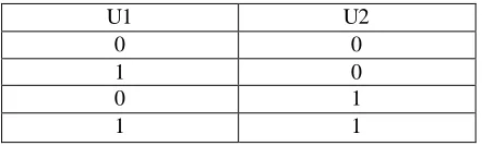
Table 1.Commited Schedule combinations of units
U1 U2
0 0
1 0
0 1
1 1
Page | 5 Table.2 Experimental Variation of Incremental Cost with Load demand and distribution of loads between
generating units
Lamda(Rs/MWh) Load
MW U1(MW) U2(MW)
35 40 20 20
49 60 20 39
49 90 27 62
49 120 45 76
52 150 61 89
59 200 100 100
59 210 95 116
60 220 100 120
63 230 105 124
63 240 115 125
65 250 125 125
In table 2.,optimized value of Incremental cost is estimated under different load demands with subjected to optimium load distribution between two units. As the load demand tends to increase, unit 2 is subjected to more load bearing capacity.Unit 2 achieves its maximum limit prior to unit 1 at load demand of 240 MW or more.Incremental cost tends to vary in step size as load demand increases as seen in Fig 4.
Table.3 Experimental Variation of Total Cost with equal IC and equal distribution of loads between generating units including SC
Total Cost with
SC(Rs/hr)
Equal Load Sharing
Cost(Rs/hr) with SC
89 89
91.5 93.5
100.9 100.25
108 107
116.05 113.75
125 125
128 127.25
130 129.5
132 131.75
136 134
136.5 136.5
In table 3, experimental values shows that upto 90 MW load demand,IC rule for sharing of load results in minimum total cost including SC.Beyond 90 MW,equal sharing of load results in total minimum cost.Both Units U1 and U2 should share equal load for the total cost to be minimized.Here SC is fixed at 10 MW.With little variation in SC for two units,sharing of load may be different for the cost to be minimized.
Test Result
For load demand upto 90 MW,LM rule should be followed .Beyond 90 MW,equal sharing of load should be done to minimize the total cost.
Fig 3. Distribution of Loads between U1 and U2
In fig.3, U2 tends to bear more load than U1 as in starting ,incremental cost for U1 is high. To reach that level of IC,U2 has to bear more load.When U1 is at 25MW,U2 is at 60 MW.U2 continues to bear more load as the load demand increases as per the slope of between interval (25-100MW for U1).
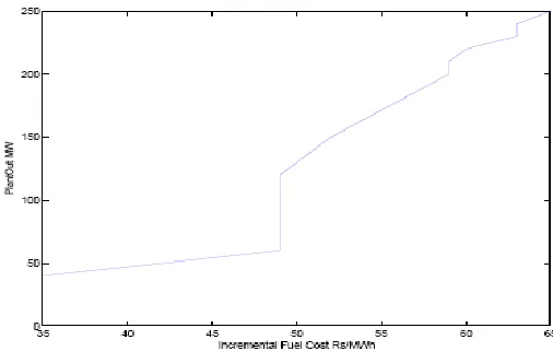
Fig 4.Variation of Incremental Cost(IC) vs Plant output
In Fig.4,IC tends to vary sharply as per the slope when load demand is low.When load demand increases,IC increases in step size as given in table 2.
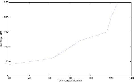
Page | 7 Fig 6. Variation of Plant output with Unit output (U2)
In fig.5 and 6,U2 is having less slope as compared to U1 with variation in load demand.U1 is increasing linearly till near to its maximum limit.U2 experienced sharp rise in slope when power demand jumps above 80 MW as given in table 2 till the optimized sharing of load above 150MW.
Fig 7. Variation of Total cost based on IC with Load Demand
Fig 8. Variation of Total cost based on equal sharing of load with Load Demand
CONCLUSION
different load demands. Different SCs for different loads can be incorporated to optimize the total cost. Combinations of Thermal and Hydro plant can be used as per the load demand and the impact of start up cost. With small step size of deltalamda, more accuracy can be observed although computation time and memory are involved. Future work incorporates artificial intelligence including more constraints in this technique.
REFERENCES
[1]. Meyer, W.W. and V.D. Albertson, .Improved Loss Formula computation by optimally ordered Enumeration Techniques',,IEEE Transmp As, 1971,9 0: 716.
[2]. Hill, E.F. and W.D. stevenson, J.R., ..A New Method of Determining Loss Coefficients", IEEE Trans. pAS, July 196g, g7: 154g.
[3]. Agarwal, S'K. and I.J' Nagrath," Optimal Scheduling of Hydrothermal Systems,,, Proc. IEEE, 1972, 199: 169.
[4]. Aytb, A'K' and A.D. Patton, "Optimal Thermal Generating Unit Commitment,,,IEEE Trans., July-Aug 1971, pAS_90: 1752.
[5]. Dopazo, J'F. et al., "An optimization Technique for Real and Reactive power Allocation", Proc, IEEE, Nov 1967. 1g77. [6]. Happ, H.H., "Optimal power Dispatch-A Comprehensives urvey”IEEE Trans. 1977, PAS-96: 841.
[7]. Harker, 8.c., "A primer on Loss Formula", AIEE Trans,95g, pt
[8]. Kothari, D.p., "Optimal Hydrothermal Scheduling and Unit commitment,. Ph. D. Thesis, B.I.T.S, Pilani, 1975.
[9]. Kothari, D.P. and I.J. Nagrath,"Security Constrained E conomic T hermal Generating Unit Commitment,, J.I.E. (India), Dec. 197g, 59: 156.
[10]. Nagrath,I .J. and D.P. Kothari, "Optimal Stochastic Scheduling of Cascaded Hydrothermal Systems", J.I.E. (India), June 1976, 56: 264.
[11]. Billinton,R., Power System Reliability Evaluation, Gqrdon and Breach, New york,1970.
[12]. Billirrton, R., R.J. Ringlee and A.J. Wood. Power System Reliabitity Calculations,The MIT Press, Boston, Mass, 1973. [13]. Kusic, G.L., computer Aided Power system Analysis, prentice-Hall, Nerv Jersey, 1986.
[14]. Kirchmayer,L .K., Economic operation of Power systems” J, ohn wiley, Newyork,
[15]. D.P Kothari and I.J NAgrath”Modern Power System Analysis”Third editions,TataMcgrawHill,2003
[16]. M. Bavafa, H. Monsef and N. Navidi, “A New Hybrid Approach for Unit Commitment Using Lagrangian Relaxation Combined with Evolutionary and Quadratic Programming”, 2009.
[17]. Peterson, W. L. and Brammer, “A capacity based Lagrangian relaxation unit commitment with ramp rate constraints”, IEEE Trans. On Power Systems 10(2): 1077-1084.
[18]. Wang, C. and Shahidehpour, S. M. 1994, “Ramp rate limits in unit commitment and economic dispatch incorporating rotor fatigue effect”, IEEE Trans. Power Systems 9(3): 1539- 1545, 1994.
[19]. Svoboda, A. J.; Tseng, C. L.; Li, C.; and Johnson, R. B. “Short term resource scheduling with ramp constraints”. IEEE Trans. Power Systems12(1): PP.77-83,1997
[20]. Abdul-Rahman, K. H.; Shahidehpour, S. M.; Aganaic, M.; and Mokhtari, S., A practical resource scheduling with OPF constraints. IEEE Trans. Power Systems 11(1): 254- 259, 1996.
[21]. Xiaohong Guan, Qiaozhu Zhai and Alex Papalexopoulos, “Optimization Based Methods for Unit Commitment: Lagrangian Relaxation versus General Mixed Integer Programming”, 2003.
[22]. A. Cohen and V. Sherkat, „Optimization Based Methods for Operations Scheduling,” Proceedings of IEEE, Vol. 75, No. 12, 1987, pp. 1574-1591.
[23]. L. A. F. M. Ferreira, T. Anderson, C. F. Imparato, T. E. Miller, C. K. Pang, A. Svoboda, and A. F. Vojdani, “Short-Term Resource Scheduling in Multi-Area Hydrothermal Power Systems”, Vol. 11. No. 3, , pp. 200-212, 1989.
[24]. X. Guan, E. Ni, R. Li, P. B. Luh, “An Algorithm for Scheduling Hydrothermal Power Systems with Cascaded Reservoirs and Discrete Hydro Constraints”, Vol. 12, No. 4, pp 1775-1780, Nov. 1997.
[25]. I. Shaw, “A Direct Method for Security Constraints Unit Commitment”,IEEE Trans.,Vol.10, No. 3, pp.1329-1339,Aug. 1995.
[26]. R. Baldick, “Generalized Unit Commitment Problem,” IEEE Transactions on Power Sys., Vol. 10, No. 1, pp. 465-473, Feb. 1995.