Please cite this article as: M. Ghomi-Avili, S. G. Jalali Naini, R, Tavakkoli-Moghaddam, A. Jabbarzadeh, A Network Design Model for a Resilient Closed-loop Supply Chain with Lateral Transshipment, International Journal of Engineering (IJE), TRANSACTIONS C: Aspects Vol. 30, No. 3, (March 2017) 374-383
International Journal of Engineering
J o u r n a l H o m e p a g e : w w w . i j e . i rA Network Design Model for a Resilient Closed-loop Supply Chain with Lateral
Transshipment
M. Ghomi-Avilia, S. G. Jalali Nainia, R, Tavakkoli-Moghaddam*b, A. Jabbarzadeha
a Department of Industrial Engineering, Iran University of Science and Technology, Tehran, Iran
b School of Industrial Engineering and Engineering Optimization Research Group, College of Engineering, University of Tehran, Tehran, Iran
P A P E R I N F O
Paper history:
Received 04 January 2017
Received in revised form 26 January 2017 Accepted 09 February 2017
Keywords:
Closed-loop Supply Chain Disruption: Resilience Strategies Uncertainty
A B S T R A C T
This paper develops a model for the closed-loop supply chain network design with disruption risk. By considering supply disruption, two factors including extra inventory and lateral transshipment are used as resilience strategies. The main purpose is to reduce the supply chain costs due to the location decisions, quantity of products between different levels and lost sale. Disruption in a supply is assumed completely by different scenarios, and then the problem is formulated by a mixed-integer programming model. Furthermore, a two-stage stochastic approach is implemented to tackle uncertainty. Finally, a sensitivity analysis is carried out to examine the effects of the resilience strategies on the structure of the supply chain and to propose some managerial insight for using the model in real world situations.
doi: 10.5829/idosi.ije.2017.30.03c.07
1. INTRODUCTION1
The supply chain network design is of great importance and can simply impact on the efficiency and effectiveness of any company. It includes strategic decisions on the number, location, capacity and commission of the production–distribution facilities of the company [1].The aim of the supply chain design is dramatically to reduce the purchasing, production, transportation, location and other associated costs. The suitable supply chain network design causes an optimum structure that makes it easy to manage the chain efficiently. An integrated forward and reverse supply chain network is one of the main fields of the logistics network design. Based on environmental, legal, social and economic factors, the reverse logistic and closed-loop supply chain has received great attentions among colligates.
During recent years, different kinds of unpredictable events (e.g., terroristic actions, disaster and some other similar events) took place to show that the world is increasingly uncertain and vulnerable. Moreover, it
1*Corresponding Author’s Email: [email protected] (R, Tavakkoli-Moghaddam)
seems that supply chains are more fragile due to plurality of industries, decentered production, reduction in a number of suppliers and focusing on deduction of inventory. Although different industries have decreased supply chains costs, but make them open to risks and disruptions simultaneously [2]. Supply chain failures are unplanned events that disrupt the normal flow of products and materials; thus, companies inside the supply chain become more susceptible to financial and operational risks consequently. While the closed-loop supply chain network (CLSCN) design has gained great attentions by researchers and practitioners during last decades, most of the existing models in the literature ignore disruption risks while configuring the CLSCN.
will effect on the business such as sudden changes in purchasing costs, interest rate, currency rate and safety regulations ruled by governmental agencies. Supply chain resilience is concerned with the system ability to return to its original state or to a new and more desirable one after experiencing a disturbance and avoiding occurrence of failure modes. In other words, the supply chain resilience is not only the ability to maintain control of the system over performance variability when encountering disturbance, but also a property of being adaptive and capable of sustained response to sudden and significant shifts of environment in the form of uncertain demands.
In order to the importance of the disruptions subject, this paper assumes that existing suppliers in a closed-loop supply chain have complete disruption in a way that they will lose all of their capacity consequently and they cannot satisfy the customer's demands on the appropriate time. In addition, for decreasing the disruption impact on the performance of the supply chain, two resilience strategies are proposed and their advantages are investigated.
The remainder of this work is organized as follows. The first section includes an introduction about the closed-loop supply chain and risks underlying. The second part related literature will be reviewed and mathematical model is being presented in the third section. The forth section deals with some numerical examples and sensitivity analysis. In the last section, conclusion and future studies will be examined.
2. LITERATURE REVIEW
In this section, a brief review on the most relevant models for the closed-loop supply chain network design problem is presented in two separate complementary research streams: the closed-loop supply chain network design and the models developed for dealing with disruption risks. As the first attempts for designing a closed-loop supply chain, Berman et al. [3] proposed a model to design a supply chain network, in which the facility disruption probabilities are not identical. They have implemented both several exact and heuristic solution methods for analyzing the impact of the
disruption probabilities on co-location and
centralization of facilities. Salema et al. [4] tried to generalize the model proposed by Fleischmann et al. [5] and presented a model for designing reverse networks and presented a general model using a stochastic mixed-integer programming approach. Then, Listeş and Dekker [6] proposed a scenario-based stochastic programming model for designing an integrated forward/reverse supply chain network and used a decomposition method to solve the model for large-scale instances based on a branch-and-cut method.
Then, Lu and Bostel [7] considered a bi-level location problem with three types of facilities that should be located in a remanufacturing network. They presented a mixed-integer programming (MIP) model that considers both forward and reverse flows and proposed a lagrangian-based heuristic algorithm to solve it. Then, for improving the service level of a supply chain network, a new lateral transshipment policy was implemented by Lee et al. [8]. Yücesan [9] presented an
effective pooling mechanism by introducing
transshipment methods, which incorporated the replenishment lead times.
Pishvaee et al. [10] presented a bi-objective mixed-integer linear programming (MILP) model that maximizes the network responsiveness and minimizes the total costs in a CLSCN. They used a memetic algorithm to solve their model. Then, Pishvaee et al. [11] proposed a robust optimization model for handling the inherent uncertainty of input data in a CLSCN design problem. First, a deterministic MILP model was developed for designing a CLSCN. Then, the robust counterpart of the proposed model was presented by using the recent extensions in robust optimization theory. Qiang et al. [12] examined a CLSCN with the decentralized decision-makers consisting of raw material suppliers, retail outlets, and the manufacturers that collect the recycled product directly from the demand market.
Amin and Zhang [13] investigated a bi-objective CLSCN that includes multiple plants, collection centers, demand markets, and products. To this aim, a MILP model proposed for minimizing the total costs. Kamali et al. [14] tried to solve the CLSCN model via determisnistic and metaheuristics namely genetic algorithm, particle swarm optimization, differential evolution and artificial bee colony. Özceylan et al. [15] described an integrated model that simultaneously optimizes the strategic and tactical decisions of a CLSCN. The main goal of this problem is to minimize costs including transportations, purchasing, refurbishing and operating the disassembly workstations costs. Also, a mixed-integer non-linear programming (MINLP) model was described for the problem. Demirel et al. [16] proposed an MIP model for a CLSCN with multi-periods and considered two policies, namely secondary market pricing and incremental incentive policies. To solve the model in real sizes, a genetic algorithm was developed. Yadegari et al. [17] presented an integrated forward/reverse logistics model, while considering three kinds of transportation modes. They proposed a memetic algorithm to solve the model.
of locations, transportations, and inventory, respectively. This system is subject to random supply disruptions that may occur at either the supplier or the retailer. Peng et al. [19] proposed a model for designing a reliable network performed after failure like a normal condition (without disruption) as much as possible. Jabbarzadeh et al. [20] presented a model for designing a resilient supply chain by considering major disruptions and interruptions in both supply and demand sides.
Vahdani et al. [21] presented a model for designing a reliable network of facilities in a CLSCN under uncertainty. For this purpose, a bi-objective mathematical programming model was developed, which minimizes the total costs and the expected transportation costs after failure of facilities of a logistics network. To solve the model, a new hybrid solution methodology was introduced by combining a robust optimization approach, queuing theory and fuzzy multi-objective programming. Then, Hatefi and Jolai [22] suggested a robust and reliable model for an integrated forward-reverse logistics network design that simultaneously takes uncertain parameters and facility disruptions into account. The proposed model was formulated based on a robust optimization approach to protect the network against uncertainty. The proposed network was single-period, single-product and multi-echelon which include production and distribution centers in the forward flow and collection, recovery and disposal centers in the reverse flow.
Esmaeilikia et al. [23] studied new methods for improving the supply chain flexibility to deal with operational risks. They assumed a supply chain includes suppliers, production and distribution centers with final customers and solved their model by simulation based optimization method. Madadi et al. [24] presented a quality-based model that effects the total disruption of supply chain. In this paper reduction of tainted raw materials by producer is investigated. They presented a single-period, single-product supply chain to prevent sending tainted materials. They implemented an efficient heuristic and meta-heuristic for solving the proposed mixed-integer stochastic model. In order to solve the proposed model, a modified version of Benders’ decomposition was applied.
Hatefi et al. [25] proposed a model for reliable design of an integrated forward-reverse logistics network and used reliability concepts to deal with facility disruptions. Unreliable hybrid facilities were allowed to be partially disrupted but they could still serve their customers with their remaining capacities. To compensate the lost capacity at unreliable facilities, a sharing strategy was also considered.
Namdar et al. [26] proposed a model for designing a reliable distribution network with limited capacity under partial and complete disruption which has been
developed by Lee et al. [8] considering different mitigation strategies. Same as Lee et al. [8], Avci and Selim [27] considered a multi-agent system model to propose a novel preventive lateral transshipment strategy with both considering demand and supply uncertainties. Hasani and Khosrojerdi [28] studied an MIP model to design a robust global supply chain considering six resilience strategies for mitigating disruption risks. They also developed a Taguchi-based memetic algorithm to determine an appropriate set of neighborhood structures. Finally, the proposed model was used for a real medical device manufacturer to prove its application.
As it can be seen from the literature, a majority of existing papers around CLSCN did not consider disruption and unavailability of facilities in their model and they considered that facilities are always available. Moreover in few studies, the supply chain's disruption has been considered to be handled by resilience concept. Thus, in this paper, a CLSCN is considered that some levels of this chain are disrupted by the natural disaster or human events, and then a model is proposed capable enough to deal it by sourcing disruption risk to make a resilient supply chain.
3.PROBLEM DEFINITION
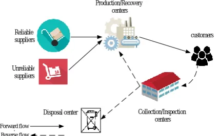
A CLSCN is considered that includes suppliers, production, collection, disposal centers and customers. The structure of the proposed CLSCN is depicted in Figure 1.
In the proposed CLSCN design, determining the optimal locations of production and collecting centers with respect to the known customer zone locations and the best flow of products in the CLSCN is of high importance in a way that the total cost of location, inventory and transportation is minimized. Moreover for preventing the effects of probable disruptions the concept of resilience strategies are implemented.
Reliable suppliers
Collection/Inspection centers Disposal center
Production/Recovery centers
customers
Unreliable suppliers
Forward flow Reverse flow
It is assumed that the raw materials are transferred from suppliers to the production centers and then by considering the operational and setup time after assembling and final manufacturing they will be delivered to the customers due to their demands. On the other hand, returned products are sent to collecting centers by considering returning policies and in these sections the products are disassembled and categorized in two groups, namely the recyclable and unrecyclable units that have their special operation time. Recyclable units are returned to a production section and implemented in the production process again. Otherwise, they are sent to the disposal center with other unrecyclable units. The model considered to be multi-period and single product when all the returned products should be conveyed to the collecting centers.
The main objective of this problem is to determine the location of production and collecting centers with the quantity of products transferring between the facilities. It has been assumed that the supplier will have some other disruptions in addition to natural disasters or human events, so this make him unable to serve the customers and then it will face complete disruptions in which their capacity will be reduced consequently. Moreover in this paper, to the best of our knowledge, for the first time with considering several resilience strategies such as keeping extra inventory and having lateral transshipment the concept of resilience strategy have been pondered in closed loop supply chain network design. For resilience strategies, using extra inventrory both in material or final product will prevent disruption in production processes and facing shortage consequently. Using lateral transshipment is in a way that when an unreliable supplier disrupts completely and is unable to serve the considered amount of material, by having transshipment among reliable and unreliable suppliers the required amount of materials will be supplied and will help to improve the service level of the proposed closed-loop supply chain and make it more resilient simultaneously.
4. MODEL FORMULATION
The model involves the following sets, parameters and decision variables:
Sets
Set of suppliers
h
Set of reliable suppliers
i
Set of unreliable suppliers
i
Set of production centers
j
Set of collection and disassembling centers
l
Set of customers
k
Set of unrecyclable units
n
Set of recyclable units
m
Set of scenarios
s
Set of time periods
t
Parameters
Probability of each scenario
s
Transportation cost from supplier i to production center j per recyclable unit of type m
ijm
a
Transportation cost from supplier i to production center j per unrecyclable unit of type n
ijn
a
Transportation cost from production center j to customer k per unit of product
jk
b
Transportation cost from customer k to collection center l
kl
c
Capacity of unreliable supplier i per unrecyclable unit of type n
in
cap
Holding cost of recyclable units in collecting center l
l
ho
Fixed cost of opening production center j
j
e
Fixed cost of opening collection center l
l
f
Disassembling cost in disassembly center l
l
g
Assembling cost in production center j
j
u
Capacity of collection center l
l cap
Capacity of unreliable supplier i per recyclable unit of type m
im
cap
Demand of customer k
k
d
Returned product's rate from customer k
k
r
Mean disposal fraction of recyclable units in each collecting center
Is equal to one if the supplier i under scenario s in period t disrupts otherwise 0
s it
Is equal to one if supplier i having complete disruption under scenario s otherwise 0
s i
Usage of recyclable unit type m in each product
m
Usage of unrecyclable unit type n in each product
n
Penalty of every dissatisfied demand for customer k
k
Holding cost of inventory for assembling in production center j
j
ho
Decision Variables
Equal to 1 if production center j is opened otherwise 0
j
op
Equal to 1 if collecting center l is opened otherwise 0
l
oc
Recyclable quantity of type m transported from supplier i to production center j at period t under scenario s
s ijmt
x
Unrecyclable quantity of type n transported from supplier i to production center j at period t under scenario s
s ijnt x
Recyclable quantity of type m transported from reliable supplier ito production center j at period t under scenario s
s i jmt
xr
Unrecyclable quantity of type n transported from reliable supplier ito production center j at period t under scenario s
s i jnt
xr
Quantity of products transported from production center j to customer k at period t under scenario s
s jkt
y
Quantity of products transported from customer k to collecting center l at period t under scenario s
s klt
w
Quantity of unrecyclable units of type n transported from collecting center l to disposal center at period t under scenario s
s ln t
z
Quantity of recyclable units of type m transported from collecting center l to production center j at period t under scenario s
s ljmt
z
Quantity of recyclable units of type m in collecting center l at period t under scenario s
Quantity of recyclable units of type m transported from collecting center l to disposal center at period t under scenario s
s lmt
z
The amount of dissatisfied demand of customer k at period t under scenario s
s kt
ls
Inventory of recyclable units type m in production center j at period t under scenario s
s jmt
In
Inventory of unrecyclable units type n in disposal center j at period t under scenario s
s jnt
In
Inventory at collecting center l under scenario s at period t
s lt
In
Equal to 1 if reliable supplier i transships unrecyclable units type n to unreliable supplier i at period t under scenario s oteherwise 0
s i int
TR
Equal to 1 if reliable supplier i transships recyclable units type m to unreliable supplier i at period t under scenario s oteherwise 0
s i i m t
TR
Equal to 1 if unreliable supplier i assigned to production center j for suppling unrecyclable units type n at period t under scenario s oteherwise 0
s ijnt
v
Equal to 1 if unreliable supplier i assigned to production center j for suppling recyclable units type m at period t under scenario s oteherwise 0
s ijmt
y
4.1. Mathematical Model
(1)
Min j j l l
j l
s s s s
ijm ijmt ijn ijnt i jm i jmt i jn i jnt
i j m t i j n t i j m t i j n t
s s
jk j jkt kl l klt
j k t k l t
s ljm ljmt l j m t
s s s s
ln ln t lmt k kt
l n m t k t
z e Op f Oc
a x a x a xr a xr
b u y c g w o z
o z z ls ho
s s
j jmt jnt j m n t
s l lt l m t
In In ho In
s.t. (2) s sm klt lmt k
w z
( l L, m M , s S , t T )(3) s s
n klt ln t k
w z
( l L, n N , s S , t T )(4)
s s
lm t lm t
z
z
( l L, m M , s S , t T )(5)
(1 ) s s
lmt ljmt j
z z
( l L, m M, s S t T)(6)
s s jkt kt kt j
y ls d
( k K , s S , t T )(7)
s s klt k jkt l L j
w r y
( k K , s S , t T )(8)
Min
s s s
ijmt i jmt ljmt
i i l
s
jkt
k
s s
ijnt i jnt
i i
m
n
1
x xr z
Y 1 x xr ,
( j J , m M , n , s S , t T )
(9)
1
s s s s
ijmt ijmt ljmt jkt
i I m i I m l m k
s s
jmt jmt x xr z Y
In In
j J , s S , m m )
( t T ,
(10)
1
s
ijnt
i I n i I n
s s s s
jnt jnt ijnt jkt
k
x
In In xr Y
j J , s S , n N )
( t T ,
(11)
1
s s s s s
lt lt klt lmt ln t
k K j m j n
In In w z z
l L, s S ,
( t T )
(12) j j
s s
jnt jmt cap op
In In ( j J , s S , t T )
(13)
s
lt l l
In cap Oc ( l L, s S, t T )
(14)
s
i jmt i m j
xr cap
( i I , m M, s S , t T )(15)
s
i jnt i n j
xr cap
,
( i I , n N s S , t T )
(16)
s s s s s i int it ijnt ijnt ijnt
i j
TR ( 1 v ) x x
,
( i I , s S t T , n N )
(17)
s
s s s si i mt it ijmt ijmt ijmt
i j
TR ( 1 y )x x ,
( i I , s S t T , m M )
(18)
s s s i i n t ijnt ijnt in i j
TR x v cap
,
( i I , s S t T , n N )
(19)
s s s
i i m t ijmt ijmt im
i j
TR x y cap
,
( i I , s S t T , m M )
(20)
s s
ijnt in ijnt
j j
x cap v
,
( i I , n N , s S t T )
(21)
s s
ijmt im ijmt
j j
x cap y
,
( i I , m M , s S t T )
(22)
0 1
j l
s s s s ijnt ijmt i int i i m t
(23)
0
s s s s s s s s s s s s s s
ijmt ijnt i jmt i jnt jkt klt lnt ljmt lmt lmt kt jmt jnt lt
x ,x ,xr ,xr , y ,w ,z ,z ,z ,z ,ls ,In ,In ,In
The objective function (1) aims to reduce the total costs, in which the first term shows the fixed costs of opening production centers and the next one refers to the cost of transporting recyclable units from suppliers to the production centers. The other terms include contract costs with reliable suppliers, transportation cost of unrecyclable units from suppliers to production centers, assembly cost in production centers, transportation cost of products from production centers to customers, costs of returning products from costumers to the collection centers and then to the disposal and production centers, demands penalty costs and costs of holding inventory, respectively. Constraint (2) shows the quantity of recyclable products in collecting centers. Equation (3) displays the quantity of unrecyclable products in collecting centers. Constraint (4) refers to the quantity of returned products that cannot be recycled and will be transferred to disposal center. Constraint (5) represents the quantity of returned products from customers that can be recycled and transferred from collecting centers to the production centers. Constraint (6) deals with satisfying demands. Constraint (7) refers to the limitation of returned products.
Constraint (8) evaluates the quantity of production in these centers. Constraints (9) to (11) explain the inventory balance limitations in production and distribution centers for recyclable and unrecyclable products. Constraints (12) and (13) state the capacity of production and distribution centers. Constraints (14) and (15) show the maximum capacity of reliable supplier for suppliyng both recyclable and unrecyclable units. The following constraints have been considered for resilience strategy. Equations (16) and (17) show that when facing disruption, lateral transshipments will support the flow of raw material shipped from suppliers to the production centers. Constraints (18) and (19) state that all transmitted material from suppliers to the production centers is equal to their capacity. Constraints (20) and (21) mean that the total received quantity of unrecylable (recyclable) units doesn't violate admission capacity of production centers. Constraints (22) and (23) state the binary conditions and non-negativity of decision variables, respectively.
4. 2. Model Linearization As it is obvious in the
model constriants, two continuous and binary variables are multiplied, and so the model is nonlinear. For linearization of the model, we use a novel approach using some concepts introduced by Vidal and Goetschalckx [29]. In this approach, another continuous variable is introduced by multiplying those binary and continuous variables. For example in Equations (18) and
(19), s
vijnt, yijnts , xijnts and xijnts are multiplied to each
other and the following set of constriants should be replaced to solve the problem.
s s
i i n t ijnt in
i j
,
( i I , s S t T , n N )
TR z cap
(24)
s ijmt
s vijnt
z M
(25) s
ijmt
s ijmt
s xijnt
s s
xijnt ( 1 vijnt) M
,
( i I , j J t T , n N , s S )
z
z
s s
i i m t ijmt im
i j
,
( i I , s S t T , n N )
TR z cap
(26)
s ijmt s ijmt s ijmt
s yijnt s xijnt
s s
xijnt ( 1 yijnt) M
,
( i I , j J t T , n N , s S )
z M
z
z
(27)
So, by replacing each nonlinear constraint with the new set of constraints, the model is linearized and ready to be solved.
5. COMPUTATIONAL EXPERIMENTS
To assess the performance of the proposed model, a computational study is considered and tested. Then, the related results are reported in this section. The model is solved by GAMS 24.3/CPLEX and with random data then the sensitivity analysis is done as follows:
5. 1. Model Validation To validate the accuracy of
the model, it is solved with GAMS/ CIPLEX by random data. The following results are achieved by solving the model with these sizes: H 3,I 2,I 5,J 2,
3
L ,K 5,N 3,M 4,S 5,T 3,Q 3.
TABLE 1.Validation test on the inventory cost parameters
E
x
p
er
ime
n
t
Holding cost (per unit of
Product)
Total inventory hold in
each period Total hold
invemtory
1 2 3
1 30 98.73 88.76 69.4 355.917
2 33 98.52 76.22 96.7 345.644
3 36 77.78 64.74 97.5 325.938
4 39 66.86 73.52 85.71 302.462
5 42 81.54 67.33 54.38 285.674
6 45 73.59 31.21 97.24 261.287
5. 2. Considering the Lateral Transshipment for a
Resilience Strategy As it can be seen in Figure 2
and Table 2, considering lateral transshipment decreases the objective function costs significantly. The reason is that, when a production center is disrupted, it will not be able to satisfy the customer’s demand, and because the penalty of dissatisfied demands is very high, the production center will incur large losses. However, by responsing to their demands through unaffected facilities with lateral transshipment, the penalty cost and consequently the total costs will decrease significantly.
5. 3. Forward or Closed-Loop As known before,
in a CLSCN, the used products are taken back to the supply chain through collection centers. This fact will have a significant effect on costs. Because supplying raw materials from mines or other suppliers are more costly than reusing the products. Figure 3 is a proof to this fact. We also investigate the effects of varying different parameters of the model on the strategic and operational costs of the supply chain. The parameters under investigation include the returned products and production capacity.
Figure 1. Differences between considering and not considering the lateral transshipment startegy
TABLE 2. Analysis on the resilience strategy
Example
Close loop costs with transshipment
(Millions)
Close loop costs without transshipment
(Millions)
Percentage of difference
1 7309 5610 23.25
2 7128 5633 20.97
3 7355 5996 18.47
4 7642 6370 16.64
5 7716 6671 13.55
6 7824 6755 13.67
7 8034 6923 13.83
8 8354 6924 17.12
9 8792 7265 17.37
10 9733 7589 22.03
Figure 3. Comparison between the forward and closed-loop supply chain
5. 4. Sensitivity Analysis on Returned Products
Figure 4 and Table 3 show that an increase in the quantity of returned products leads to an increase in the operational costs (e.g., transportation, inventory and penalty).
Conversely, it results in a considerable decrease of the strategic cost (e.g., fixed opening cost of facilities and total cost of the supply chain). It means that a company can save significant costs by improving the utilization of returned products from the customers.
5. 5. Sensitivity Analysis on Production Capacity
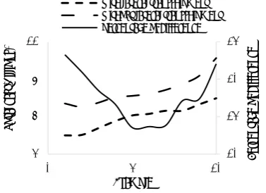
By increasing the production capacity at production centers, the total cost will be decreased. It should be noted that increasing the production capacity needs to spend costs. However, the increased production capacity causes less strategic and operational costs because of less production facility numbers, which incur a reductioon in total costs. This issue can be seen in Figure 5.
10 15 20 25
5 7 9 11
0 5 10
Example
P
er
ce
nt
ag
e o
f
di
ff
er
enc
e
To
tal
c
as
t(
B
ill
io
ns
)
with lateral transshipment without lateral transshipment percentage of difference
0.00 5.00 10.00 15.00 20.00
0 2 4 6 8 10
T
otal
C
os
t(
M
il
li
o
n
s)
Examples
Figure 4. Impacts of varying the quantity of the returned products on the strategic and operational costs of the supply chain
TABLE 3. Impacts of varying the quantity of the returned products on the strategic and operational costs of the supply chain
Returned product
objective function (Millions)
strategic costs (Millions)
operational costs (Millions)
30000 72.5 13.0 59.5
35000 68.3 13.0 55.3
40000 63.5 13.0 50.5
45000 58.8 26.7 32.1
50000 49.6 26.7 22.9
55000 45.3 26.7 18.6
60000 42.3 26.7 15.6
Figure 5. Changes of the total cost by changing the production capacity
6. CONClUSION
Nowadays, disruption and demolition has great effects on the performance of supply chains. This paper deals with the problem of closed loop supply chain with
supply risk that aims to reduce supply costs due to the location decisions, quantity of products between supply chain levels and lost sale. In this paper, to the best of our kowledge the resilience and flexibility concept has been presented with supply risk in closed loop supply chain design by considering lateral transshipment and keeping extra inventory then some sensitivity analyses has been done on the proposed model to evaluate its efficiency. The effects of disruption, other parametes such as production capacity and implementing resilience strategies on the closed loop supply chain have been showed by the results of analysis. Proposing exact solution methods for solving the model in large scale can be a challenging scope for future study. In addition, the model can be extended by considering quality engineering for dividing returned products and improving final products features, having multiple decision makers in closed loop network and the concept of game theory. Moreover, robust programming can be an efficient tool for dealing with uncertainty in supply chain to make the model more flexible and strong enough to mitigate uncertainties.
7. REFERENCES
1. Melo, M.T., Nickel, S. and Saldanha-da-Gama, F., "Facility location and supply chain management–a review", European Journal of Operational Research, Vol. 196, No. 2, (2009), 401-412.
2. Li, J., Wang, S. and Cheng, T.E., "Competition and cooperation in a single-retailer two-supplier supply chain with supply disruption", International Journal of Production Economics, Vol. 124, No. 1, (2010), 137-150.
3. Berman, O., Krass, D. and Menezes, M.B., "Facility reliability issues in network p-median problems: Strategic centralization and co-location effects", Operations Research, Vol. 55, No. 2, (2007), 332-350.
4. Salema, M.I.G., Barbosa-Povoa, A.P. and Novais, A.Q., "An optimization model for the design of a capacitated multi-product reverse logistics network with uncertainty", European Journal
of Operational Research, Vol. 179, No. 3, (2007), 1063-1077.
5. Fleischmann, M., Beullens, P., BLOEMHOF‐RUWAARD, J.M. and Wassenhove, L.N., "The impact of product recovery on logistics network design", Production and Operations
Management, Vol. 10, No. 2, (2001), 156-173.
6. Listeş, O. and Dekker, R., "A stochastic approach to a case study for product recovery network design", European Journal of
Operational Research, Vol. 160, No. 1, (2005), 268-287.
7. Lu, Z. and Bostel, N., "A facility location model for logistics systems including reverse flows: The case of remanufacturing activities", Computers & Operations Research, Vol. 34, No. 2, (2007), 299-323.
8. Lee, Y.H., Jung, J.W. and Jeon, Y.S., "An effective lateral transshipment policy to improve service level in the supply chain", International Journal of Production Economics, Vol. 106, No. 1, (2007), 115-126.
9. Yücesan, E., "Stochastic optimization for transshipment problems with positive replenishment lead times", International
Journal of Production Economics, Vol. 135, No. 1, (2012),
61-72. 0.0
5.0 10.0 15.0 20.0 25.0 30.0
0 10 20 30 40 50 60 70
30000 35000 40000 45000 50000 55000 60000
str
ateg
ic
c
os
ts
(
M
il
lio
n
s)
ope
ra
ti
on
al
c
os
ts
(
M
il
li
o
ns
)
Quantity Of Returned Products
operational costs strategic costs
95.00 96.00 97.00 98.00 99.00 100.00 101.00
0.00 100.00 200.00 300.00 400.00 500.00
30 50 70
P
rof
it(
M
il
li
o
n
s)
T
otal
c
os
t(
M
il
li
o
n
s)
10. Pishvaee, M.S., Farahani, R.Z. and Dullaert, W., "A memetic algorithm for bi-objective integrated forward/reverse logistics network design", Computers & Operations Research, Vol. 37, No. 6, (2010), 1100-1112.
11. Pishvaee, M.S., Rabbani, M. and Torabi, S.A., "A robust optimization approach to closed-loop supply chain network design under uncertainty", Applied Mathematical Modelling, Vol. 35, No. 2, (2011), 637-649.
12. Qiang, Q., Ke, K., Anderson, T. and Dong, J., "The closed-loop supply chain network with competition, distribution channel investment, and uncertainties", Omega, Vol. 41, No. 2, (2013), 186-194.
13. Amin, S.H. and Zhang, G., "A multi-objective facility location model for closed-loop supply chain network under uncertain demand and return", Applied Mathematical Modelling, Vol. 37, No. 6, (2013), 4165-4176.
14. H. R. Kamali, A.S., M. A. Vahdat-Zad, H. Khademi-Zare, "Deterministic and metaheuristic solutions for closed-loop supply chains with
continuous price decrease", International Journal of Engineering
Transactions C, Vol. 27, No. 12, (2014), 1897-1906.
15. Özceylan, E., Paksoy, T. and Bektaş, T., "Modeling and optimizing the integrated problem of closed-loop supply chain network design and disassembly line balancing", Transportation Research Part E: Logistics and Transportation Review, Vol. 61, No., (2014), 142-164.
16. Demirel, N., Özceylan, E., Paksoy, T. and Gökçen, H., "A genetic algorithm approach for optimising a closed-loop supply chain network with crisp and fuzzy objectives", International
Journal of Production Research, Vol. 52, No. 12, (2014),
3637-3664.
17. Yadegari, E., Najmi, H., Ghomi-Avili, M. and Zandieh, M., "A flexible integrated forward/reverse logistics model with random path-based memetic algorithm", Iranian Journal of
Management Studies, Vol. 8, No. 2, (2015), 287.
18. Qi, L., Shen, Z.-J.M. and Snyder, L.V., "The effect of supply disruptions on supply chain design decisions", Transportation
Science, Vol. 44, No. 2, (2010), 274-289.
19. Peng, P., Snyder, L.V., Lim, A. and Liu, Z., "Reliable logistics networks design with facility disruptions", Transportation
Research Part B: Methodological, Vol. 45, No. 8, (2011),
1190-1211.
20. Jabbarzadeh, A., Fahimnia, B., Sheu, J.-B. and Moghadam, H.S.,
"Designing a supply chain resilient to major disruptions and supply/demand interruptions", Transportation Research
Part B: Methodological, Vol. 94, (2016), 121-149.
21. Vahdani, B., Tavakkoli-Moghaddam, R., Modarres, M. and Baboli, A., "Reliable design of a forward/reverse logistics network under uncertainty: A robust-m/m/c queuing model", Transportation Research Part E: Logistics and Transportation
Review, Vol. 48, No. 6, (2012), 1152-1168.
22. Hatefi, S. and Jolai, F., "Robust and reliable forward–reverse logistics network design under demand uncertainty and facility disruptions", Applied Mathematical Modelling, Vol. 38, No. 9, (2014), 2630-2647.
23. Esmaeilikia, M., Fahimnia, B., Sarkis, J., Govindan, K., Kumar, A. and Mo, J., "A tactical supply chain planning model with multiple flexibility options: An empirical evaluation", Annals of
Operations Research, (2014), 1-26.
24. Madadi, A., Kurz, M.E., Mason, S.J. and Taaffe, K.M., "Supply chain design under quality disruptions and tainted materials delivery", Transportation Research Part E: Logistics and
Transportation Review, Vol. 67, (2014), 105-123.
25. Hatefi, S., Jolai, F., Torabi, S. and Tavakkoli-Moghaddam, R., "A credibility-constrained programming for reliable forward– reverse logistics network design under uncertainty and facility disruptions", International Journal of Computer Integrated
Manufacturing, Vol. 28, No. 6, (2015), 664-678.
26. J. Namdara, R.T.-M., H. Rezaei-Soufib, N. Sahebjamnia*c, "Designing a reliable distribution network with facility fortification and transshipment under partial and complete disruptions", International Journal of Engineering
Transactions C, Vol. 29, (2016), 1273-1281.
27. Avci, M.G. and Selim, H., "A multi-agent system model for supply chains with lateral preventive transshipments: Application in a multi-national automotive supply chain",
Computers in Industry, Vol. 82, (2016), 28-39.
28. Hasani, A. and Khosrojerdi, A., "Robust global supply chain network design under disruption and uncertainty considering resilience strategies: A parallel memetic algorithm for a real-life case study", Transportation Research Part E: Logistics and
Transportation Review, Vol. 87, (2016), 20-52.
29. Vidal, C.J. and Goetschalckx, M., "A global supply chain model with transfer pricing and transportation cost allocation",
European Journal of Operational Research, Vol. 129, No. 1,
A Network Design Model for a Resilient Closed-loop Supply Chain with Lateral
Transshipment
M. Ghomi-Avilia, S. G. Jalali Nainia, R, Tavakkoli-Moghaddamb, A. Jabbarzadeha
a Department of Industrial Engineering, Iran University of Science and Technology, Tehran, Iran
b School of Industrial Engineering and Engineering Optimization Research Group, College of Engineering, University of Tehran, Tehran, Iran
P A P E R I N F O
Paper history:
Received 04 January 2017
Received in revised form 26 January 2017 Accepted 09 February 2017
Keywords:
Closed-loop Supply Chain Disruption: Resilience Strategies Uncertainty
ديكچ ه
یم هتخادرپ نیمات کسیر طیارش رد هتسب هقلح نیمات هریجنز هکبش یحارط هلئسم یسررب هب ،هلاقم نیا رد رد رب هولاع .دوش
نا نینچمه و یفاضا یدوجوم زا هدافتسا لیبق زا یلماوع ،نیمأت رد للاتخا نتفرگ رظن یاه یژتارتسا ناونع هب یضرع لاقت
فاطعنا یم هتفرگ رظن رد یریذپ ،یبای ناکم تامیمصت هب هجوت اب هریجنز یاه هنیزه ندرک هنیمک هلئسم نیا فده .دنوش
م هب فلتخم یاهویرانس کمک هب ناگدننک نیمات رد للاتخا .دشاب یم هتفر تسد زا شورف و حوطس نیب نایرج نازی
یم هتفرگ رظن رد لماک تروص یم لدم هتخیمآ حیحص ددع یزیر همانرب هدافتسا اب هلئسم .دوش
درکیور زا نینچمه و دوش
م رد تیعطق مدع نتفرگ رظن رد یارب یلامتحا یا هلحرم ود یم هدافتسا یداهنشیپ لد
تیساسح لیلحت زین ،همتاخ رد .دوش
ماجنا نیمات هریجنز راتخاس یور رب )یریذپ تشگرب( یروآ بات یاه یژتارتسا تاریثات یسررب روظنم هب لدم یور رب
یم یم هئارا یعقاو یایند رد لدم زا هدافتسا روظنم هب یتاداهنشیپ سپس و دوش .دوش