A 3d Micro-Plane Model for Shape Memory Alloys

(1)

A 3D MICRO-PLANE MODEL FOR SHAPE MEMORY

ALLOYS

A. Roohbakhsh Davaran* and S.A. Sadrnejad

Department of Civil Engineering, K.N. Toosi University of Technology P.O. Box 15875-4416, Tehran, Iran

[email protected] - [email protected]

*Corresponding Author

(Received: October 8, 2007 - Accepted in Revised Form: November 22, 2007)

Abstract To assess the thermo-mechanical behavior of shape memory alloys and analyzing these

special materials, a simple constitutive integrated model, named micro-plane, is proposed. The model deals with shear and normal on plane stress/strain components and also on plane shear orientation as well. The proposed simple model is capable of predicting three-dimensional behavior as the superposition of on plane elastic and inelastic deformations. In the case of static constraint, two on plane stress/strain components and corresponding orientations could be obtained by transferring the stress/strain tensor. Then to calculate the on plane deformations, a plane constitutive law is needed to assess unknown strains/stresses. To represent the capability of this model, the predicted different test data across time and temperature domainsare compared with the experimental results. In these test results the shape memory alloys behavior as: super elasticity under various temperatures, loading rate effects, asymmetry in tension and pressure, various loops of loading and unloading, hydrostatic pressure effects, different proportional tension-shear biaxial loading and unloading and also deviation from normality due to non-proportional tension-shear biaxial loading and unloading, are investigated and presented. The interesting well accuracy of results proves the strength and capability of the proposed model.

Keywords Shape Memory Alloys, Shape Memory Effect, Super Elasticity, Micro-Plane, Multi-Laminate

ﻩﺪﻴﻜﭼ

ﻭﺭﺍﺩﻪﻈﻓﺎﺣﯼﺎﻫﮊﺎﻴﻟﺁﯽﮑﻴﻧﺎﮑﻣﻮﻣﺮﺗﺭﺎﺘﻓﺭﯽﺳﺭﺮﺑﺭﻮﻈﻨﻣﻪﺑ

ﻥﺎﮑﻣﺍ ﻞﻴﻠﺤﺗ ﯼﺩﺪﻋ ﮏـﻳﺹﺎـﺧﺩﺍﻮﻣﻦﻳﺍ

ﯼﺍﻪﺤﻔﺻﺰﻳﺭﺵﻭﺭﺱﺎﺳﺍﺮﺑﻩﺩﺎﺳﯼﺭﺎﺘﻓﺭﯼﻮﮕﻟﺍ ﺮﺑ

ﺱﺎﺳﺍ ﻭﺩﺎﻬﻨﺗ

ﻭﺵﺮﺑﻭﺩﻮﻤﻋﻪﻔﻟﻮﻣ

ﺩﺍﺪﺘﻣﺍ

ﺭﺩﺵﺮـﺑﻪﻔﻟﻮﻣ

ﺖﺳﺍﻩﺪﺷﻪﺋﺍﺭﺍﺎﻬﻧﺁﻦﻴﺑﻂﺑﺍﻭﺭﻭﻪﺤﻔﺻﺰﻳﺭ

.

ﯽﻣﻩﺪﺷﻪﺋﺍﺭﺍﯼﻮﮕﻟﺍ

ﺗ ﻪﻠﻴـﺳﻭﻪـﺑﺍﺭﻪـﻄﻘﻧﮏﻳﯼﺪﻌﺑﻪﺳﺭﺎﺘﻓﺭﺪﻧﺍﻮ

ﺭﺎﺛﺁﻊﻤﺟ

ﺪـﻨﮐﯽـﻨﻴﺑﺶﻴﭘﻒﻠﺘﺨﻣﯼﺎﻳﺍﻭﺯﺎﺑﻪﺤﻔﺻﻦﻳﺪﻨﭼﺭﺩﻞﮑﺷﺮﻴﻴﻐﺗﯽﻄﺧﺮﻴﻏ

.

ﯽﮑﻴﺗﺎﺘـﺳﺍﺪـﻴﻗﺖـﻟﺎﺣﺭﺩ

ﯽﻣﺖﺳﺩﻪﺑﻪﺤﻔﺻﺰﻳﺭﻥﺎﻤﻫﺭﺩﺶﻨﺗﺭﻮﺴﻧﺎﺗﻝﺎﻘﺘﻧﺍﺯﺍﻪﺤﻔﺻﺰﻳﺭﺮﻫﺭﺩﺩﻮﺟﻮﻣﯼﺎﻫﻭﺮﻴﻧ

ﻪﺒﺳﺎﺤﻣﯼﺍﺮﺑﺲﭙﺳﺪﻳﺁ

ﻓﻪﺤﻔﺻﺰﻳﺭﺮﻫﺭﺩﻞﮑﺷﺮﻴﻴﻐﺗﺥﺮﻧ

ﯽﻣﻡﺯﻻﯼﺭﺎﺘﻓﺭﻥﻮﻧﺎﻗﮏﻳﻂﻘ

ﺪﺷﺎﺑ . ﻮـﮕﻟﺍﻦﻳﺍﺖﻴﻠﺑﺎﻗﻭﯽﻳﺎﻧﺍﻮﺗﯽﺑﺎﻳﺯﺭﺍﯼﺍﺮﺑ

ﺖﺳﺍﻩﺪﺷﻪﺴﻳﺎﻘﻣﻢﻫﺎﺑﯽﺑﺮﺠﺗﻭﯽﻠﻴﻠﺤﺗﺞﻳﺎﺘﻧ

.

ﯼﺭﺍﺩﻪـﻈﻓﺎﺣﻪـﻳﺍﺭﺍﺭﺩﻮﮕﻟﺍﯽﻳﺎﻧﺍﻮﺗﺞﻳﺎﺘﻧﻦﻳﺍﺭﺩ

ﺎـﻣﺖﻴـﺻﺎﺧﻭ

ﯽﻋﺎﺠﺗﺭﺍﻕﻮﻓ

ﻒﻠﺘﺨﻣﯼﺎﻫﺎﻣﺩﺭﺩ

ﯼﺭﺍﺬﮔﺭﺎﺑﺥﺮﻧﺮﻴﺛﺎﺗ

- ﺶﺸﮐﻭﺭﺎﺸﻓﺭﺩﯽﻧﺭﺎﻘﺘﻣﺎﻧ

ﻞﻴﮑﺸـﺗ

ﯼﺎـﻫﻪـﻘﻠﺣ

ﯼﺭﺍﺬﮔﺭﺎﺑﺭﺩﯼﺭﺍﺩﺮﺑﺭﺎﺑﻭﯼﺭﺍﺬﮔﺭﺎﺑﺮﺛﺍﺭﺩﯽﻠﺧﺍﺩ

ﺩﺍﻮﻣﻦﻳﺍﺭﺎﺘﻓﺭﻭﮏﻴﺗﺎﺘﺳﺍﻭﺭﺪﻴﻫﺭﺎﺸﻓﺮﺛﺍﻭﯼﺭﻮﺤﻣﮏﻳﯼﺎﻫ

ﺪﻣﺎﻌﺗﺯﺍﻑﺍﺮﺤﻧﺍﺖﻴﺻﺎﺧﻦﻴﻨﭽﻤﻫﻭﺐﺳﺎﻨﺘﻣﯽﺷﺮﺑﻭﯽﺸﺸﮐﯼﺭﻮﺤﻣﻭﺩﯼﺭﺍﺬﮔﺭﺎﺑﺖﺤﺗ

ﺭﺩ ﺮﺛﺍ

ﺪﻨﭼﯼﺭﺍﺬﮔﺭﺎﺑ

ﺐﺳﺎﻨﺘﻣﺎﻧﯼﺭﻮﺤﻣ

ﯼﺭﺍﺬﮔﺭﺎﺑﺭﺩ

ﺮﺠﺗﺞﻳﺎﺘﻧﺎﺑﯼﺭﻮﺤﻣﺪﻨﭼﯼﺎﻫ

ﺖﺳﺍﻩﺪﺷﻪﺴﻳﺎﻘﻣﯽﺑ

ﯽـﻣﻥﺎﺸﻧﻪﮐ

ﻪـﺑﺞﻳﺎـﺘﻧﺪـﻫﺩ

ﻢﻫ،ﻮﮕﻟﺍﻦﻳﺍﺯﺍﻩﺪﻣﺁﺖﺳﺩ

ﺪﻧﺭﺍﺩﯽﺑﺮﺠﺗﺞﻳﺎﺘﻧﺎﺑﯽﺑﻮﺧﯽﻧﺍﻮﺧ

. ﺯﺍﻩﺪـﺷﻪﺘﺧﺎـﺳﯼﺎـﻫﻩﺯﺎﺳﺭﺎﺘﻓﺭ،ﯼﺩﺎﻬﻨﺸﻴﭘﯼﻮﮕﻟﺍ

ﻞﮑﺷﺮﻴﻴﻐﺗﻝﺎﻤﻋﺍﻪﺧﺮﭼﺭﺩﺍﺭﺭﺍﺩﻪﻈﻓﺎﺣﺕﺍﺰﻠﻓ

ﯽﻣﺎﻫ

ﯽﻨﻴﺑﺶﻴﭘﯽﺒﺳﺎﻨﻣﺭﻮﻃﻪﺑﺪﻧﺍﻮﺗ

ﺪﻳﺎﻤﻧ .

1. INTRODUCTION

Nowadays, civil engineers in addition to taking the factors such as capability of the structure for enduring different loads into account, pay special attention to designing more precise structures with

larger spans or reducing the mass of constructional materials in order to economic justification of their projects. Maintenance and reinforcement of the existing buildings is one of the most responsibilities of civil engineers.

(2)

control systems has engaged researchers worldwide. To this end, civil engineers are after using constructional materials with better specifications than the ones currently used. Shape memory alloys are one of such materials which are also called intelligent materials. Although these materials have been known decades ago, but they have been used in the building construction recently. These materials like many other metals have more than one crystal structure which is called poly crystal. The shape of crystal structure in these materials is dependent on temperature and external tension imposed on them [1].

The structural phases in high and low temperatures are respectively called austenite and martensite. The ability to transform into each other in different tensions and temperatures and consequently change of mechanical and electrical properties of these materials has encouraged researchers to use these alloys in smart structures. To date, some 30 types of these alloys have been known, but due to the common temperature of structures and observing economic justification issues, only some of them are applicable [1]. The ability of returning into the initial shape through increasing the temperature after pseudo plasticity transformations in low temperature phases is one of the most distinctive features of these alloys. To this reason, these alloys are called shape memory alloys and this phenomenon is called pseudo plasticity [1].

Another notable phenomenon is super elasticity which is also called pseudo elasticity. Increase of the tension imposed on material in fixed temperature will turn the austenite phase into martensite phase and after unloading the martensite phase will be turned into austenite phase. The high capacity for energy damping in hysteretic loops is another feature of these alloys. For further study on application of these alloys in building construction industry, refer to [1].

So, analysis of these materials is of high importance in designing and for analysis of the structures in which these alloys have been utilized, a suitable behavioral constitutive law is required. A three-dimensional model based on the micro-plane integrated method has been proposed as a more capable model predicting the special behavioral aspects of memory alloys in this paper. In continuation, first, the micro-plane method has

been described, then the on plane constitutive law cast in micro-plane framework has been introduced and in the next section, comparison of the predicted results with experiments have been presented.

2. MICRO-PLANE MODEL

2.1. Brief History

This model was initially

proposed by Taylor [2]. He suggested that the constitutive behavior of polycrystalline metals are explained by the relations between strain and tension vectors in planes with different orientations in which the macroscopic stress and strain tensors are obtained by sum of all the vectors in these planes using some static and kinematic constraints and formula. Batdorf, et al [3] were the first individuals who expanded the idea of Taylor and developed a realistic model for plasticity properties of polycrystalline alloys. Many other researchers have modified this method for alloys. Meanwhile, this method has been used for development of the non-linear hardening properties in soils and stones. Micro-plane is referred to a plane in materials with different orientation which is used for estimation of the microstructure behavior of materials. After extension of the micro-plane model by Prat, et al [4] for estimation of damages arising from compression and tension, a very more effective formula for concrete was introduced by Bazant [5,6].

The micro-plane formula for anisotropic clays and for soils has been introduced by Prat, et al in [7-9], respectively.

Details of micro-plane formula in both static and kinematic constraints can be seen in the studies of Bazant, et al [10]. For each formula, in static and kinematic constraints, properties of material are identified by using stress and strain relations in micro-planes.

2.2. The Model Specifications

The

(3)

Figure 1. The shear stress path in a micro-plane in the

proportional loading and unloading cases and thermo-mechanical borders of crystal phase transformation.

Figure 2. The shear stress path in a micro-plane in the

non-proportional loading and unloading cases and thermo-mechanical borders of crystal phase transformation.

phenomenological model which aims to obtain the mechanical macroscopic behavior of materials divided into sampling plane behaviors. Accordingly, the constitutive law is defined based on plane stress/strain tensors; while in a micro-plane investigate material behavior in several planes with different orientations which are called micro-plane, so that this method is much closer to fit the assessment of mechanical behavior of a group of crystals with multi side reactions instead. For an isotropic material, the constitutive laws in micro-planes can be considered equal for different planes as well as material parameters. Although, we should note that the number and orientation of micro-planes are obtained using numerical methods and the micro-planes should not be necessarily based on crystallographic structure of materials (like some microstructure mechanical models), but it is possible to select micro-planes according to the planes with known orientation based on crystallographic for a shape memory alloy and apply micro-plane model directly in single crystal microstructure scale [11]. Overall behavior of polycrystalline materials is the sum of shear effects in the planes with different orientation related to the single crystal grains [11]. In macro-scale or polycrystalline scale, the micro-plane model is used as a method with the ability to be turned from a constitutive law in each micro-plane to a three-dimensional macro-scale model for stress-strain tensor. In this case, orientation of micro-planes can be selected using numerical considerations.

Below considerations have been assumed for facilitating the development of the model:

• Negligibility of thermal expansion

• Elasticity of volumetric strain

For obtaining shear strains and their orientations in the micro-plane, it is required that a constitutive law to be defined in each micro-plane. In this model defines a 2-D thermo-mechanic phase transformation surface for on planes constitutive law.

The martensitic strain tensor in macro-scale are due to summation of shear displacement in micro-scale between grains [11], so a constitutive law for each micro-plane has been considered which its 2-D phase transformation surfaces are dependent on

the shear direction and the vertical component in the micro-planes (Figure 1,2).

(4)

Sadjadpour, et al [12,19,20] and applied some amendments to change it into a 3-D constitutive law. The main advantage of this model is the possibility of definition of independent constitutive law for each micro-plane. Also, the model has the capacity to describe complicated phenomena like deviate from normality that can not be described by using macro-scale models based on associated flow rule or J2 invariant [11]. For example, McDawell, et al [13] experimentally showed that the constitutive laws which are based on J2 such as the yielding surface of Von Mises and Drucker Prager are not suitable for non-proportional 2-D loading. McDawell, et al [13] and McNaney, et al [15] using experiments on shape memory alloys under axial torsion non-proportional loading. The obtained results proved that opposite the model based on J2 formula, in non-proportional loading, martensite strains are not in the same direction with shear stresses. This phenomena called deviate from normality (vertex effect) [11].

2.3. Constitutive Law Based on Static

Constraint

In this method the stress components

in each micro-plane are obtained by transforming of the macro-scale stress tensor of σij in the

micro-plane. So, first the strain components of each plane are obtained using the constitutive law of the micro-plane and then the macro-scale strain tensor is obtained using the virtual work principle [11]. Stress components could be obtained as below:

j n ij

σ

i

T = (1)

j n i n ij

σ

N

σ = (2)

i n N σ i T si

σ = − (3)

Ti is the component of stress tensor in plane and ni

is component of unit normal and σN is the vertical

component of stress tensor and σsi is the shear

components of stress tensor in each micro-plane. Based on the virtual work principle:

∫ +

+ ∫

=

Ω

)dΩ ri δ j n rj δ i (n 2 Sr ε 2π

3

Ω

dΩ j n i n N ε 2π

3 ij

ε (4)

Ω is the surface of the unit hemisphere.

Equation 4 has been derived based on the fact

that the virtual work inside the hemisphere and external surface is equal which has been precisely obtained by Bazant. Integral of the said equation can be derived using numerical methods of Gaussian integral with a series of points over the surface of the hemisphere. This method uses a limited series of micro-planes with different orientations for every point.

3. CONSTITUTIVE LAW ON MICRO-PLANE

The proposed constitutive law for plane has been developed upon modification of the one dimensional constitutive law presented by Sadjadpour, et al [12,19,20]. The prominent modification of this constitutive law is defining a thermo-mechanical boundary for transformation on each plane that depends on the correspond orientation of shear stress path.

3.1. Kinetic Law

It is supposed that in each

micro-plane, the shear strain can be divided into elastic, martensite and plastic as below:

t) (x, ps ε t) (x, ms t)ε

λ(x,

t) (x, es ε t) (x, s

ε = + + (5)

In this equation, ε_s is the total shear strain term in each micro-plane and λε_ms is the shear strain related to the martensite phase in each micro-plane and ε_es is the elastic shear strain term in each micro-plane and ε_ps is the plastic shear strain in each micro-plane. λ represents the stress-temperature induced martensitic fraction on plane which varies between zero and one and ε_ms is the maximum shear strain of crystal fraction in the micro-plane that is defined as follows:

⎥⎦ ⎤ ⎢⎣

⎡

∈ εc_ms,εt_ms

ms

ε and

λ

∈

[ ]

0,1 (6)

(5)

to the micro-plane is only included in elastic transformations: t) (x, en ε t) (x, n

ε =  (7)

3.2. Constitutive Law

The relation between

shear stress and shear strain in the micro-plane is defined as follows:

) ms λε ps ε s (ε s E s

σ = − − (8)

)) 0 θ θ Ln( (1 p C cr θ λ

η= l − + (9)

cr θ ) cr θ (θ

ω(θ)=l − (10)

ω(θ)

ms ε s σ

dλ= − (11)

s

λσ

m

dε =  (12)

s

σ

p

dε = (13)

and the transformation in each micro-plane is defined as: ⎪ ⎪ ⎪ ⎪ ⎪ ⎩ ⎪⎪ ⎪ ⎪ ⎪ ⎨ ⎧ > − < − − − − + − < + > − − + − + + = otherwise 0 0 λ , dλ dλ p 1 ) 1 dλλ (dλ (1 λ 1 λ , dλ dλ p 1 ) 1 ) dλ (dλ (1 λ λ & & & (14) In the above equations Es is the shear elasticity

module in micro-plane, σs is the shear stress

component in micro-plane, η is the entropy density, _l is the latent heat of transformation, θcr is

the thermodynamic transformation temperature, Cp

is the heat capacity (assumed to be equal in both the austenite and martensite), θ0 is the initial

temperature, θ is the current temperature, ω(θ) is the difference of chemical energy between

austenite and martensite phases, dλ is the driving force associated with the volumetric fraction in each micro-plane, dεm is the driving force

associated with the martensite strain in each micro-plane and dεp is the driving force associated with

the plastic strain in each micro-plane.

Parameters λ&+, λ&−, dλ+, dλ− are respectively the determiner of the slope of the loop in stress-strain curve in loading path, determiner of slope of the loop in unloading path, determiner of the start point of phase transformation from austenite to martensite and determiner of the start point of phase transformation from martensite to austenite.

The term ε&_m which is defined as the indicator of all the phenomena related to phase transformation such as twining, variants and detwining, the below equations are given:

⎪⎩ ⎪ ⎨ ⎧ ⎥⎦ ⎤ ⎢⎣ ⎡ ∈ = = = otherwise 0 t m ε , c m ε m ε ασ

λεm αd ) m ε λ, , εm (d εm K m ε& (15)

α is the parameter related to the material.

For ε&_p an equation dependent to the loading rate is defined:

⎪⎩ ⎪ ⎨ ⎧ _≥ _≤₋ = = = other 0 yt σ orσ yt σ σ H σ H εp d ) y σ , εp (d εp K p ε & & (16)

H is the hardening parameter and σyt is the yielding

shear stress. For the temperature changes the below equation is given:

) cr θ p C ) ) 0 λ ) t ( λ ( ( exp 0 θ (t)

θ = − l (17)

In each micro-plane the relations are as follows: p i C m i C e i C i

(6)

⎥ ⎥ ⎥ ⎥

⎦ ⎤

⎢ ⎢ ⎢ ⎢

⎣ ⎡

=

I G

1 0

0 I E

1 e i

C (19)

⎥ ⎦ ⎤ ⎢ ⎣ ⎡ ⋅ =

α

0 0 0

λ

m i

C & (20)

⎥ ⎥ ⎦ ⎤ ⎢ ⎢ ⎣ ⎡ =

H 1 0

0 0 p i

C (21)

T i T i C i T i

Cˆ = ⋅ ⋅ ₍₂₂₎

⎥ ⎥ ⎦ ⎤ ⎢ ⎢ ⎣ ⎡ ∂ ∂ =

σi

σ i

T (23)

∑

= ⋅

= 13

1 i Wi Ci 8π

C ˆ ₍₂₄₎

In the above equations, EI and GI are respectively

the tensional and shear elasticity modules in the micro-plane and Ci is the compliance matrix in

each micro-plane and Ce_i , C_im, Cp_i are the elasticity, phase transformation and plasticity compliance matrixes in each micro-plane respectively Cˆ_i_{is the transformed compliance} matrix related to the ith_{plane. T}

i is the

transformation matrix that transforms micro strain from micro-plane to macro-scale strain tensor. σi is

the stress matrix in micro-plane and σ is the stress tensor in macro-scale. Wi are the weight

coefficients related to the integral Equation 4 by numerical method over the surface of the hemisphere [14].

3.3. Parameters

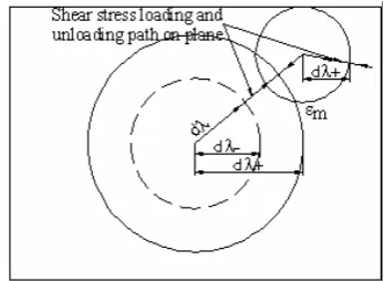
dλ+

and

dλ−

Parameters dλ+

and dλ− determine the starting point of phase transformation in a micro-plane. This has been shown in the Figure 1. In this figure, the shear path has been shown in a micro plane. Two eccentric circles with the radius dλ+ and dλ− are indicators of thermo-mechanical limits of austenite and martensite phase transformations. The radiuses of

these circles depend on the shear paths (22 and 23). to the extent that the thermo-mechanical path of stress does not exit the circledλ+, the strain is in the elastic and linear limits. As soon as the loading path passes the border of circle, martensite strains (εm) are started until it reaches the amount of λ to 1

in the micro-plane. In the unloading path, the strains will be linear until the reverse path of shear stress enters the circle dλ−. In this case, the martensite strains start to return until the value of λ reaches from one to zero. In such case, all the martensite strains will return to zero. Continuing unloading the strains will return to elastic and linear case until it reaches to the initial condition i.e. zero stress and zero strain.

Values of dλ+ and dλ− which indicate the starting points of phase transformation in the cases of loading and unloading respectively, are given as follows:

) Ms ( ω ) a ( f

dλ+ = (25)

) As ( ω ) a ( g

dλ− = (26)

in the above equations, As and Ms are the temperatures in which the transformation to austenite and martensite phase are started when the external tension is zero. f(a) and g(a) are the coefficients of micro-planes which are function of the orientation of shear stress component micro-planes (a) which has been introduced in the Section 5-2.

In the case which loading and unloading are not monotonic, i.e. the loading path change (Figure 2), at the moment of change in shear stress path in a micro-plane dependent on the angle of the direction change, another thermo-mechanical border circle to the center of the starting point of path change and the radius of the new dλ+ can be assumed.

4. DEMONSTRATION

(7)

stress history σ11 = A sin ωt and then conduct a

parameter study and present capability of model. According to the studies on a type of NiTi alloy conducted by McNaney, et al [15], parameters of material can be considered as follows:

Ms = 51.55˚C As = -6.36˚C

12.3(J/gr) =

l C_p =837J/kgok

2.5% m

c

ε =− εm_t =5%

65GPa

E= σ_y=1500MPa

Using Equations 10, 22 and 23, it leads to the following relations:

⎟ ⎠ ⎞ ⎜

⎝ ⎛

+ − =

+

Ms As

As Ms f(a)

dλ _l

⎟ ⎠ ⎞ ⎜

⎝ ⎛

+ − =

−

Ms As

Ms As g(a)

dλ l (27)

2 Ms As cr

θ = + (28)

Now, with regard to the single axis tension as σ11 =

A Sin ωt in which A = 1300 MPa and, ω = 2π/T and T = 5×10-3_{s, the initial conditions are as}

follows:

ε(0) = 0 εp(0) = 0 εm(0) = 0

λ(0) = 0 θ(0) = 0

After comparing the results with the experiments given by McNaney [15], the parameters obtained for the material are as follows:

a = 0 α = 5.65 f(0) = 1 P = 2 g(0) = -0.4 H = E/50

0.1 λ

λ&+ =−&−=

It should be mentioned of A < σy, so we will not

enter the plastic strain limits. The responses resulted from micro-plane model have been shown in the Figure 3.

As loading started in an elastic state until it reaches the northwest point in the upper loop. Here, the phase transformation from austenite to martensite begins, so the slope of the curve changes. Then, it reaches the north east point in the upper loop in which the phase transformation is completed and reaches the phase of martensite completely. Again by increase of the load, it returns to the elastic state and the slope of the cure reaches the initial slope.

In the unloading path, the curve returns with this slope until it reaches to the southeast point. Here, the martensite phase begins to change to austenite phase. Continuing unloading the material is completely turned into austenite phase and it reaches to south west point in the upper loop. Then it reaches again in linear-elastic term until the tension and strain reaches zero. Similarly, for the compression loading, a loop is formed, but the tensional loop is a little different from compression loop. This phenomenon proves the asymmetry in tension and compression of alloys which can be seen in this model.

Figure 4 shows the comparison between uniaxial stress and strain which has been derived from the experimental studies conducted by Mc Naney and the curve obtained from micro-plane model.

Parameters of materials are as the same of the abovementioned ones, except for E = 40 GPa and

l = 8.3(J/g).

It can be clearly seen that all the curves are coincidence, only slope of curves in the reverse path is a little different in the linear-elastic term, this is due to the fact that in this model it has assumed that the elasticity module is constant in both austenite and martensite phase. It can be changed easily.

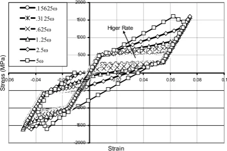
4.1. Loading Rate

Figure 5 shows the

(8)

-2000 -1500 -1000 -500 0 500 1000

-0.06 -0.04 -0.02 0 0.02 0.04 0.06 0.08 Strain

St

re

ss

(M

Pa

)

Start A→M

Finish A→M

Start M→A Finish M→A

Start A→M Start M→A

Figure 3. A typical curve of stress-strain obtained from the

micro-plane model during a harmonic loading cycle.

0 50 100 150 200 250 300 350 400 450 500

-0.01 0 0.01 0.02 0.03 0.04 0.05 0.06 0.07

Strain

St

re

ss

(M

Pa

)

Simulation Experiment

Figure 4. Comparison between micro-plane model and

experimental data obtained by McNaney, et al [15] as the result of uniaxial loading and unloading.

-2000 -1500 -1000 -500 0 500 1000 1500 2000

-0.06 -0.04 -0.02 0 0.02 0.04 0.06 0.08 0.1

Strain

St

re

ss

(M

P

a

)

.15625ω .3125ω .625ω 1.25ω 2.5ω 5ω

Higer Rate

Figure 5. Numerical results related to single axis

tension-strain with different rates of harmonic loading and unloading.

occurs in these curves and so an increase in the surface of loops is seen.

Also, in the higher rate of loading curve, a residual strain can be seen due to the high unloading rate. Unloading rate is so high that before the austenite phase is completed and phase transformation strains approach to zero, unloading is completed and tension reaches zero. These conditions are related to a certain stick-slip behavior that occurs due to sudden application of stresses which their corresponding strains are not fully be back after unloading. Also, in the curve related to the highest rate of loading, a softening can be seen because the loading rate is so high that before phase transformation is finished, loading reaches to pick of sinus cycle and so when unloading started, phase transformation still continues. All these results comply with experimental results [16].

4.2. Ambient Temperature and Investigating

the Shape Memory Effect

Figure 6 shows the

temperature variations effects in stress-strain curves. In this case, different environment temperatures have been assumed as the initial temperature θ0 and the same harmonic uniaxial

loading has been applied.

As it can be seen, in the curve related to the least environment temperature i.e.-70˚C the coefficient λ increases sharply to the value of 1 in which the austenite phase has been turned into martensite phase, so it is independent to the loading And εm results from rotation of variant. By

increase of environment temperature, for increase of the volumetric fraction coefficient λ, stress increasing is required till the environment temperature reached 170˚C and the phase transformation is not seen.

All the results of this model comply with results from observation and well known Clausius-Clapeyron relation [17].

Also, by investigation of curves the shape memory effects can be perceived. As the temperature reduced to-70˚C, the λ coefficient moves to reach 1 before loading but εm remains

(9)

θ=-70

-2000 0 2000

-0.06 _strain 0.04

S

tre

ss

(MP

a)

θ=-40

-2000 0 2000

-0.06 0.04

Strain

St

re

ss(

M

P

a)

θ=-10

-2000 0 2000

-0.06 _Strain 0.04

S

tr

ess(

M

P

a)

θ=20

-2000 0 2000

-0.06 _Strain 0.04

S

tr

ess(

M

P

a)

θ=50

-2000 0 2000

-0.06 _Strain 0.04

S

tre

ss

(MP

a)

θ=80

-2000 0 2000

-0.06 _Strain 0.04

Str

es

s(

M

P

a)

θ=110

-2000 0 2000

-0.06 Strain 0.04

S

tre

ss

(MP

a)

θ=140

-2000 0 2000

-0.1 0.1

Strain

Str

es

s(

M

Pa

)

θ=170

-2000 0 2000

-0.1 _Strain 0.1

S

tre

ss

(MP

a)

Figure 6. The numerical results of the effect of temperature changes

on the single axis stress-strain curves.

But if the environment temperature increases (say 20˚C), then due to loading and unloading, no residual strain remains and as can be seen in the curve related to the temperature 20˚C, the stress related to the zero strain will be zero which actually is the shape memory effect of alloys that can be seen in this behavioral constitutive law.

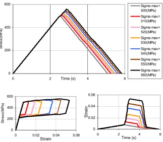
4.3. Internal Loops

Figure 7 shows the

numerical results of the micro-plane model as the result of triangular uniaxial loading and unloading. As it can be seen, in some of these curves, before completion of the phase transformations, unloading starts, so loops become smaller and return with the same slope until the reverse phase transformation starts and the strains of the phase transformation return to their initial state and the material turns to the

austenite shape. In continuation, the material returns to the same state with zero stress and strain. These curves comply with the results stated by Abeyarante, et al [18].

5. INVESTIGATION OF THE BEHAVIOR UNDER 3-D LOADING

(10)

0 200 400 600

0 2 Time (sec) 4 6

St

re

ss

(M

P

a)

Sigma max= 500(MPa) Sigma max= 510(MPa) Sigma max= 520(MPa) Sigma max= 530(MPa) Sigma max= 540(MPa) Sigma max= 550(MPa) Sigma max= 560(MPa)

0 200 400 600

0 0.02 0.04 0.06

Strain

S

tr

ess(

M

P

a)

0 0.02 0.04 0.06

0 2 4 6

Time (sec)

St

ra

in

Figure 7. The numerical results of the micro-plane model as duo to

triangular uniaxial loading and unloading.

effect of stress on the starting point of phase transformation in each micro-plane:

I E

2 N σ (a) f Ms As

As Ms f(a)

dλ ⎟+ ′

⎠ ⎞ ⎜

⎝ ⎛

+ − =

+

l

I E

2 N σ (a) g Ms As

Ms As g(a)

dλ ⎟− ′

⎠ ⎞ ⎜

⎝ ⎛

+ − =

−

l (29)

(a)

f′ and g′(a) are the functions relating to the normal stress and a is related to the shear stress path in the micro-plane.

By comparing the curves resulted by this method in the Figure 8, the overall effect of the hydrostatic stress on the behavior of these materials can be seen. The curves are related to the effective stress (σ₁₁−σ₁₁hyd) and effective strain

) 3

v ε 11

(ε − as the result of triangular loading and unloading of a material point in three cases. In the first case, without hydrostatic stress, loading as uniaxial tension stress and unloading to zero. In the second case, first the point is under hydrostatic pressure of 50MPa and then the triangular uniaxial tension stress is loaded and unloaded. In the third case, the same loading is done under the hydrostatic stress of 150MPa. In all the three cases, f′(a) and g′(a) have been considered 0.1 but these parameters can be obtained using experimental results.

As it can be seen, by increase of the hydrostatic stress, the materials starts to phase transformation in a higher tensional stress and the loop related to the phase shift moves upward. The obtained results show qualitatively the capability of model for representing the hydrostatic pressure effects on transformation in this material.

Time (s)

(11)

0 200 400 600

0 0.02_(ε 0.04 0.06

11−εv/3)

(σ11 −σ11

hy

d )(

M

pa

)

Hydrostatic Pressure=0(MPa) Hydrostatic Pressure=50(MPa) Hydrostatic Pressure=150(MPa)

Figure 8. Effects of hydrostatic stress on the effective

stress-effective strain curve obtained from micro-plane model.

-15 -10 -5 0 5 10 15

0 15 30 45 60 75 90

ALIGNMENT OF SHEAR STRESS PATH θ (Deg)

dλ + &

δλ

− M(

pa)

DLAMBDAP DLAMBDAN

Figure 9. The changes of dλ+ and dλ- relative to the angle θ.

5.2. Proportional Biaxial Loading

In this

section, the results obtained from the model for a single point of the material which is under simultaneous loading and unloading stress σ11 and

shear τ23 has been investigated in six different

cases and has been compared with experimental results obtained by McNaney, et al [15].

Six different cases of loading and unloading are as follows:

Case 1

. Maximum tensional strain ε11 equals 6 %

and maximum shear strain (torsion) ε23

equals 0 %

Case 2

equals 2 %

Case 3

equals 2 %

Case 4

. Maximum tensional strain ε11 equals 1.5

% and maximum shear strain (torsion) ε23

equals 2 %

Case 5

. Maximum tensional strain ε11 equals 0.7

% and maximum shear strain (torsion) ε23

equals 2 %

Case 6

equals 2 %

After calibration of the model with experimental results obtained by McNaney, et al [15] the values for dλ+ and dλ− in each micro-plane can be introduced as a function of a based on Equations 18 and 19 in which θ is the angles between the shear stress in each micro-plane relative to the base direction. Here, the base direction is the direction of the shear stress resulting from the axis stress σ11 in it. These functions can be seen in

the Figure 9.

In Figure 10 the obtained results have been compared with the experimental results introduced by McNaney, et al [15] in the six loading and unloading paths. As it can be seen, the results nearly coincide with each other.

5.3. Non-Proportional Biaxial Loading

In

this section, the results obtained from the model for a single point of the material has been presented in case the point is under single axis

stress in direction of σ11 and then shear stress is

applied to it in the direction of τ23 as the stress σ11

remains constant, then shear stress unloading and tensional stress unloading is applied in three cases; The first case, the maximum tensional stress is equivalent to 0.7 % of the axial strain and the shear stress is equivalent to 2 % of the shear strain. In the second case, the figures are 1.05 % and 2 % and in the third case the figures are 6 % and 2 % respectively.

(12)

Tension6%-Torsion0%

0 100 200 300 400 500

0 0.02_Strain0.04 0.06

St

re

ss

(M

P

a)

Experimental Simulation

0 100 200 300 400 500

0 0.02_Strain0.04 0.06

St

re

ss

(M

P

a)

0 100 200 300 400 500

0 0.02_Strain0.04 0.06

St

re

ss

(M

P

a)

Tension1.5%-Torsion2%

0 100 200 300 400 500

0 0.02_Strain0.04 0.06

S

tre

ss

(M

pa

)

0 100 200 300 400 500

0 0.02_Strain0.04 0.06

St

re

ss

(M

P

a)

0 100 200 300

0 0.02Strain0.04 0.06

St

re

ss

(M

P

a)

Figure 10. Comparison of the results obtained from micro-plane model with the experimental results of McNaney, et al [15] in the six paths of biaxial tensional and rotational loading and unloading.

[15], first in net rotation case and then in the three mentioned loading cases.

6. CONCLUSION

A semi-microscopic mechanical time-thermo-mechanical based model depends on loading rate, working in 3-D space developed and proposed for evaluation of shape memory alloys behavior. The micro-plane framework added this model power upon the capabilities such as applying the

(13)

Tension.7%-Torsion2%

0 100 200 300 400 500

0 0.02_Strain0.04 0.06

S

tr

ess(

M

P

a)

0 100 200 300 400 500

0 0.02 Strain0.04 0.06

St

re

ss

(M

P

a)

0 100 200 300 400 500

0 0.02 Strain0.04 0.06

St

re

ss

(M

P

a)

Figure 11. Comparison of the numerical results obtained from the micro-plane model and the experimental results of

McNaney, et al [15] for biaxial tensional and rotational loadings.

capability in prediction of the thermo-mechanical behavior of the structures manufactured from shape memory alloys.

7. REFERENCES

1. Janke, L., Czaderski, C., Motavalli, M. and Ruth, J., “Application of Shape Memory Alloys in Civil Engineering Structures-Overview, Limits and New Ideas”, Materials and Structures, Vol. 38, No. 5, (June 2005), 578-592.

2. Bragg, W. L., Desch, C. H., Taylor, G. I., Mott, N. F., Orowan, E., Da, E. N., Andrade, C., Preston, G. D. and Hatfield, W. H., “A Discussion on Plastic Flow in Metals”, Mathematical and Physical Sciences, Vol. 168, No. 934, (7 November 1938), 302-317.

3. Batdorf, S. B. and Budiansky, B., “A Mathematical Theory of Plasticity Based on the Concept of Slip”,

NACA Technical Note, Vol. 1871, (April 1949). 4. Bazant, Z. P. and Prat, P. C., “Micro-Plane Model for

Brittle-Plastic Material 1. Theory”, Journal of

Engineering Mechanics, ASCE, Vol. 114, (1988),

1672-1687.

5. Bazant, Z. P., Caner, F. C., Carol, I., Adley, M. D. and Akers, S. A., “Micro-Plane Model M4 for Concrete. I: Formulation with Work-Conjugate Deviatoric Stress”, Journal of Engineering Mechanics, ASCE, Vol. 126, (2000), 944-953.

6. Caner, F. C. and Bazant, Z. P., “Micro-Plane Model M4 for Concrete II: Algorithm and Calibration”, Journal of Engineering Mechanics, ASCE, Vol. 126, (2000), 954-961.

7. Bazant, Z. P. and Prat, P. C., “Creep of Anisotropic Clay-New Micro-Plane Model”, Journal of

Engineering Mechanics, ASCE, Vol. 113, (1987),

1050-1064.

(14)

Damage Tensor Based on Micro-Plane Model”, Journal of Engineering Mechanics, ASCE, Vol. 117, (1991), 2429-2447.

10. Carol, I. and Bazant, Z. P., “Damage and Plasticity in Microplane Theory”, International Journal of Solids and Structures, Vol. 34, (1997), 3807-3835.

11. Brocca, M., Brinson, L. C. and Bazant, Z. P., “Three Dimensional Constitutive Model for Shape Memory Alloys Based on Micro-Plane”, J. Mech. Phys. Solids, Vol. 50, (2002), 1051-1077.

12. Sadjadpour, A. and Bhattacharya, K., “A Micromechanics Inspired Constitutive Model for Shape-Memory Alloys: The One-Dimensional Case”, Smart Mat. Struct., Vol. 16, (2007), 51-62.

13. Lim, T. J. and McDowell, D. L., “Mechanical Behavior of an Ni-Ti Shape Memory Alloy Under Axial-Torsional Proportional and Nonproportional Loading”, Journal of Engineering Materials and Technology-Transaction of the ASME, Vol. 121, No. 1, (Jan 1999), 9-18.

14. Sadrnejad, S. A., “Principles of soil plasticity”, K. N. T. University, Tehran, Iran, (1999).

15. McNaney, J. M., Imbeni, V., Jung, Y., Papadopoulos, P. and Ritchie, R. O., “An Experimental Study of the

Superelastic Effect in a Shape-Memory Nitinol Alloy under Biaxial Loading”, Mechanics of Materials, Vol. 35, (2003), 969-986.

16. Nemat-Nasser, S., Choi, J. Y., Guo, W. G. and Isaacs, J. B., “Very High Strain-Rate Response of a NiTi Shape-Memory Alloy”, Mechanics of Materials, Vol. 37, (2005), 287-298.

17. Otsuka, K. and Wayman, C. M., “Shape Memory Materials”, Cambridge University Press, Cambridge, U.K., (1998).

18. Abeyaratne, R., Chu, C. and James, R. D., “Kinetics of Materials with Wiggly Energies: Theory and Application to the Evolution of Twinning Microstructure in a Cu-Al-Ni Alloy”, Phil. Mag. A, Vol. 73, (1996), 457-497.

19. Sadjadpour, A. and Bhattacharya, K., “A Micromechanics Inspired Constitutive Model for Shape Memory Alloys”, Smart Mater., Vol. 16, No. 5, (2007), 1751-1756.