THERMOHYDRODYNAMIC CHARACTERISTICS OF JOURNAL
BEARINGS RUNNING UNDER TURBULENT CONDITION
B. Maneshian and S.A. Gandjalikhan Nassab*
Department of Mechanical Engineering School of Engineering, Shahid Bahonar University P.O. Box 76169-133, Kerman, Iran
maneshian@yahoo.com - ganj110@mail.uk.ac.ir *Corresponding Author
(Received: October 14, 2008 – Accepted in Revised Form: December 11, 2008)
Abstract A thermohydrodynamic (THD) analysis of turbulent flow in journal bearings is presented
based on the computational fluid dynamic (CFD) techniques. The bearing has infinite length and operates under incompressible and steady conditions. In this analysis, the numerical solution of Navier-Stokes equations with the equations governing the kinetic energy of turbulence and the dissipation rate, coupled with the energy equation in the lubricant flow and the heat conduction equation in the bearing are obtained. The AKN Low-Re k-ε turbulence model is used to simulate the mean turbulent flow field. Considering the complexity of the physical geometry, conformal mapping is used to generate an orthogonal grid and the governing equations are transformed to the computational domain. Discretized forms of transformed equations are obtained by the control volume method and solved by the SIMPLE algorithm. In this study, cavitation effects are also considered by using an appropriate cavitation model. The liquid fraction in the cavitated region is computed based on the continuity requirements and rather than the two-phase flow of lubricant in this region, a homogenous mixture with equivalent properties is assumed and the governing equations still apply in the cavitated region. From this method, the lubricant velocity, pressure and temperature distributions in the circumferential and cross film directions are obtained without any approximation. The numerical results are compared with experimental data and good agreement is found.
Keywords Journal Bearings, Thermohydrodynamic, Infinite Length, Turbulent Flow
ﻩﺪﻴﻜﭼ
ﺱﺎﺳﺍﺮﺑ ﺩﻭﺪﺤﻣﺎﻧ ﻝﻮﻃ ﺎﺑ ﻝﺎﻧﺭﻭﮊ ﻥﺎﻗﺎﺗﺎﻳ ﺭﺩ ﻢﻃﻼﺘﻣ ﻥﺎﻳﺮﺟ ﻲﮑﻴﻣﺎﻨﻳﺩﻭﺭﺪﻴﻫﻮﻣﺮﺗ ﺰﻴﻟﺎﻧﺁ ﺮﺿﺎﺣ ﺭﺎﮐ ﺭﺩ
ﺖﺳﺍ ﻩﺪﺷ ﻡﺎﺠﻧﺍ ﻲﺗﺎﺒﺳﺎﺤﻣ ﺕﻻﺎﻴﺳ ﮏﻴﻣﺎﻨﻳﺩ ﮏﻴﻨﮑﺗ .
ﺭﺍﺪﻳﺎﭘ ﻂﻳﺍﺮﺷ ﻭ ﻢﮐﺍﺮﺗ ﻞﺑﺎﻗﺮﻴﻏ ،ﻢﻃﻼﺘﻣ ﻥﺎﻳﺮﺟ ﺖﺤﺗ ﻥﺎﻗﺎﺗﺎﻳ
ﻲﻣ ﺭﺎﮐ ﺪﻨﮐ . ﻳﺎﭘ ﺮﺑ ﺰﻴﻟﺎﻧﺁ ﺔ
ﻭﺩ ﺕﻻﺩﺎﻌﻣ ﻱﺩﺪﻋ ﻞﺣ ﻭﺎﻧ ﻱﺪﻌﺑ
ﻩﺍﺮﻤﻫ ﺲﮐﻮﺘﺳﺍﺮﻳ ﻁﻮﺑﺮﻣ ﺕﻻﺩﺎﻌﻣ ﺎﺑ
ﻭ ﻲﺸﺒﻨﺟ ﻱﮊﺮﻧﺍ ﻪﺑ
ﻓﺎﺿﺍ ﻪﺑ ﻢﻃﻼﺘﻣ ﻥﺎﻳﺮﺟ ﺭﺩ ﻱﮊﺮﻧﺍ ﻑﻼﺗﺍ ﺥﺮﻧ ﺔ
ﻟﺩﺎﻌﻣ ﺔ ﻥﺎﻗﺎﺗﺎﻳ ﺭﺩ ﻲﺘﻳﺍﺪﻫ ﺕﺭﺍﺮﺣ ﻝﺎﻘﺘﻧﺍ ﻭ ﻦﻏﻭﺭ ﻥﺎﻳﺮﺟ ﺭﺩ ﻱﮊﺮﻧﺍ
ﺖﺳﺍ ﻩﺪﺷ ﻡﺎﺠﻧﺍ .
ﻝﺪﻣ ﺯﺍ ﺎﺘﺳﺍﺭ ﻦﻳﺍ ﺭﺩ
AKN Low-Re k-ε
ﻪﻴﺒﺷ ﻱﺍﺮﺑ ﺖﺳﺍ ﻩﺪﺷ ﻩﺩﺎﻔﺘﺳﺍ ﻥﺎﻳﺮﺟ ﻱﺯﺎﺳ
. ﻪﺟﻮﺗ ﺎﺑ
ﻲﮔﺪﻴﭽﻴﭘ ﻪﺑ ﺳﺪﻨﻫ
ﺔ ﻴﺣﺎﻧ ﺎﺗ ﻩﺪﺷ ﻩﺩﺎﻔﺘﺳﺍ ﺲﻳﺪﻤﻫ ﺖﺷﺎﮕﻧ ﺯﺍ ﻦﻏﻭﺭ ﻥﺎﻳﺮﺟ ﺔ
ﻴﺣﺎﻧ ﻪﺑ ﺰﮐﺮﻣ ﻢﻫ ﺮﻴﻏ ﻩﺮﻳﺍﺩ ﻭﺩ ﻦﻴﺑ ﺔ
ﺤﻔﺻ ﺭﺩ ﻲﻠﮑﺷ ﻞﻴﻄﺘﺴﻣ ﺔ
،ﻲﺗﺎﺒﺳﺎﺤﻣ ﻭ ﻲﮑﻳﺰﻴﻓ ﺕﺎﺤﻔﺻ ﻦﻴﺑ ﻁﺎﺒﺗﺭﺍ ﻦﺘﺷﺍﺩ ﺎﺑ ﺲﭙﺳ ﻭ ﻩﺪﺷ ﻞﻘﺘﻨﻣ ﻲﺗﺎﺒﺳﺎﺤﻣ
ﻨﻣﺍﺩ ﻪﺑ ﻢﮐﺎﺣ ﺕﻻﺩﺎﻌﻣ ﺔ
ﻩﺪﺷ ﻩﺩﺍﺩ ﻝﺎﻘﺘﻧﺍ ﻲﺗﺎﺒﺳﺎﺤﻣ ﺪﻧﺍ
. ﺘﺴﺴﮔ ﻡﺮﻓ ﺔ
ﻳ ﻝﺎﻘﺘﻧﺍ ﺕﻻﺩﺎﻌﻣ ﻪﺑ ﻝﺮﺘﻨﮐ ﻢﺠﺣ ﺵﻭﺭ ﺎﺑ ﻪﺘﻓﺎ
ﻢﺘﻳﺭﻮﮕﻟﺍ ﺎﺑ ﻭ ﻩﺪﻣﺁ ﺖﺳﺩ SIMPLE
ﻩﺪﺷ ﻱﺩﺪﻋ ﻞﺣ ﺪﻧﺍ
. ،ﺐﺳﺎﻨﻣ ﻝﺪﻣ ﮏﻳ ﺯﺍ ﻩﺩﺎﻔﺘﺳﺍ ﺎﺑ ﻲﺳﺭﺮﺑ ﻦﻳﺍ ﺭﺩ ﻦﻴﻨﭽﻤﻫ
ﻳﺪﭘ ﺕﺍﺮﻴﺛﺄﺗ ﺓﺪ
ﺭﺩ ﻦﻏﻭﺭ ﻱﺯﺎﻓﻭﺩ ﻥﺎﻳﺮﺟ ﻱﺎﺟ ﻪﺑ ﻝﺩﺎﻌﻣ ﺹﺍﻮﺧ ﺎﺑ ﻦﮕﻤﻫ ﺐﻴﮐﺮﺗ ﮏﻳ ﻲﻨﻳﺰﮕﻳﺎﺟ ﺎﺑ ﻥﻮﻴﺳﺎﺘﻳﻭﺎﮐ
ﺖﺳﺍ ﻩﺪﺷ ﻪﺘﻓﺮﮔ ﺮﻈﻧ .
ﻣ ،ﺵﻭﺭ ﻦﻳﺍ ﺯﺍ ﻩﺩﺎﻔﺘﺳﺍ ﺎﺑ ﺑ ﻲﺑﻮﺧ ﺖﻗﺩ ﺎﺑ ﻦﻏﻭﺭ ﻥﺎﻳﺮﺟ ﺭﺩ ﺎﻣﺩ ﻭ ﺭﺎﺸﻓ ،ﺖﻋﺮﺳ ﻥﺍﺪﻴ
ﻪ
ﺖﺳﺍ ﻩﺪﻣﺁ ﺖﺳﺩ ؛
ﺴﻳﺎﻘﻣ ﺍﺮﻳﺯ ﺔ
ﻘﺑﺎﻄﺗ ﻲﺑﺮﺠﺗ ﻱﺎﻫ ﻩﺩﺍﺩ ﺎﺑ ﻱﺩﺪﻋ ﺞﻳﺎﺘﻧ ﻲ
ﻲﻨﺘﻓﺰﻳﺬﭘ ﻲﻣ ﻥﺎﺸﻧ ﺍﺭ ﺪﻫﺩ
.
1. INTRODUCTION
Journal bearings are used extensively where rotating machinery operates at high speed. The bearing load depends on the nature of the application. For example, in high speed gearbox applications, high loads may be imposed by the combined torque
levels and gearbox design layout, while in turbocharger applications, the requirement is to support the combined weight of the rotor and shaft only.
flow, the fluid layer exhibits regular intermixing with each other, such that this type of flow is an irregular fluid motion in which the various flow properties such as velocity and pressure show random variations with time and position.
It is clear that the lubricant flow is laminar for small values of the Reynolds number. Taylor vortices are known to occur when the Taylor number TR defined as:
s r
c
μ
c V
ρ
TR=
Reaches the value of 41.2, after which the flow breaks down to turbulence. In this expression, ρ
and μ are the fluid density and viscosity, c is the radial gap, rs is the shaft radius and V is the shaft
linear speed. Transition between vortex and turbulent flow is well known to be more gradual and can not thus be characterized by one single number. Many experiments show a wide range of 100 ≤ TR ≤ 150 for fully turbulence [1].
The lubricant flow in journal bearings under turbulent condition has been a subject of study for many years. In all of the theoretical works, the Reynolds equation was considered as the governing equation that must be solved to obtain the lubricant pressure in journal bearings. It should be noted that the Reynolds equation is an approximate form of the momentum equation that neglects the inertia term and the curvature effect in lubricant flow. The theoretical treatment of turbulent flow in bearing fluid film was first attempted by Wilcock [2] and then by Constantinescu [3], who used mixing length theory of Prandtl. Constantinescu assumed that the mean fluid inertia stresses are negligible compared to fluctuating inertia forces, known as turbulent stresses. However, at low Reynolds number, this argument may not stand, because mean fluid inertia forces may be of the same order as viscous forces. Following Prandtl’s mixing length theory; Constantinescu decoupled the different equations, which can lead to velocity expression for journal bearing. He presented the analytical expression for pressure in turbulent condition.
Nagaraju, et al [4] presented a THD solution for a finite length two-lobe journal bearing. They obtained the pressure and temperature distributions
by simultaneous solution of the generalized Reynolds equation with the energy equation for lubricant flow. In that study, the static characteristics (in terms of load capacity, attitude angle, end leakage and friction parameter) and dynamic characteristics (in terms of critical mass, threshold speed and damped frequency of whirl) were determined.
An analytical investigation of steady, incompressible and viscous flow between two eccentric rotating cylinders at high Reynolds numbers was presented by Rahimi [5]. He used singular perturbation method to solve the set of continuity and momentum equations. In that work, a modified bi-polar coordinate system was introduced with two small perturbation parameters, the eccentricity ratio and inverse of the Reynolds number, causing a singular perturbation theory treatment.
Chun [6] considered the effects of variable density and variable specific heat on maximum pressure and maximum temperature in high-speed journal bearing operation. He used the Reynolds equation for computing lubricant pressure in a steadily loaded journal bearing with infinite width under turbulent condition. Through the result of analysis, he concluded that under high speed operations, the consideration of variable density and variable specific heat on the calculation of bearing load and frictional power loss cannot be ignored.
Peng, et al [7] developed a THD model for predicting the three-dimensional temperature field in an air-lubricated journal bearing. In that study, they used simultaneous solution of the Reynolds equation and the energy equation for air flow in a gas bearing. Parametric studies covering a fairly wide range of operating speeds and load conditions were carried.
cylindrical coordinate system (r,θ,z). The finite difference forms of the governing equations were obtained using finite volume method and were solved by the SIMPLEC algorithm. By this method, the velocity, pressure and temperature distributions of lubricant flow in journal bearings were calculated. It is noted that using the cylindrical coordinate system for solving the governing equations introduces an approximation in the analysis, because this coordinate system can not match to the surface boundaries in journal bearings.
The THD analysis of laminar flow in journal bearings was done by Gandjalikhan Nassab, et al [10] using CFD technique. That work was based on the numerical solution of the full three-dimensional Navier-Stokes equation, coupled with the energy equation in the lubricant flow and the heat conduction equations in the bearing and the shaft. Considering the complexity of the physical geometry, conformal mapping was used to generate an orthogonal grid and the governing equations were transformed into the computational domain. Discretized forms of the transformed equations were obtained by the control volume method and solved by the SIMPLE algorithm.
Gandjalikhan Nassab [11] studied the effect of inertia on three-dimensional THD characteristics of journal bearings running under laminar flow. In that study, the Navier-Stokes equations were solved with and without considering the inertia terms by CFD method. It was shown that the influence of inertia increases under the condition of high Reynolds number, large clearance and small eccentricity ratio.
As noted before, all of the CFD works in obtaining the THD characteristics of journal bearings were limited under the assumption of laminar lubricant flow. On the other hand, in the cases of turbulent flow, the approximate Reynolds equations in different forms were solved by many investigators. To the best of author’s knowledge, the THD behavior of turbulent flow in journal bearings has not been obtained numerically by CFD techniques. Thereby, the present paper is the follow up of the previous study by the second author [10] in which the governing equations for turbulent flow are solved numerically by CFD method using appropriate cavitation and turbulence models.
It is evident that to simulate a turbulent flow
accurately, a precise turbulence model is required. Among the existing low-Reynolds-number k-ε
models, the model developed by Abe, et al [12], which is the AKN Low-Re k-ε turbulence model, is regarded as one of the most reliable one, which is employed in the present analysis. The model can reproduce the near-wall limiting behavior and provides accurate predictions for the boundary layer turbulent flows with favorable or adverse pressure gradients, such as for the lubricant flow in journal bearings [13].
2. GOVERNING EQUATIONS
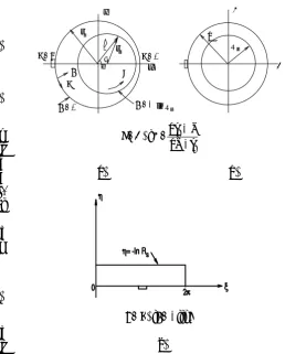
There are a number of governing equations which those that are solved simultaneously in the present study are the continuity equation, the time averaged Navier-Stokes equations, the equations of turbulent kinetic energy and its dissipation rate, the energy equation for the lubricant flow and Laplace's equation for thermal conduction in the bearing. The non-dimensional forms of these equations in the Cartesian coordinate system, Figure 1, can be written as:
x y ri rs e ω inlet oil groove
θi
Figure 1. Geometrical configuration of journal bearing.
TABLE 1. The Values of Constant Parameters.
Parameter Value
σk 1.4
σε 1.4
σT 0.9
Cμ 0.09
Cε1 1.4
Cε2 1.9
* * 1 * t Re 1 ] * y * k ) k * t 1 ( Re 1 * k * v [ * y ] * x * k ) k * t 1 ( Re 1 * k * u [ * x ε − ϕ μ = ∂ ∂ σ μ + − ∂ ∂ + ∂ ∂ σ μ + − ∂ ∂ (4) * k 2 * f 2 C * k * * 1 Re * t 1 C ] * y * ) * t 1 ( Re 1 * * v [ * y ] * x * ) * t 1 ( Re 1 * * u [ * x ε ε ε − ε ϕ μ ε = ∂ ε ∂ ε σ μ + − ε ∂ ∂ + ∂ ε ∂ ε σ μ + − ε ∂ ∂ (5) 0 ) * y B * T ( * y ) * x B * T ( *
x ∂ =
∂ ∂ ∂ + ∂ ∂ ∂ ∂ (6) * * ] * y * T ) Re T * t Pe 1 ( * T * v [ * y ] * x * T ) Re T * t Pe 1 ( * T * u [ * x φ μ = ∂ ∂ σ μ + − ∂ ∂ + ∂ ∂ σ μ + − ∂ ∂ (7) Where 2 ) * x * v * y * u ( 2 ) * y * v ( 2 2 ) * x * u ( 2 * 1 φ ∂ ∂ + ∂ ∂ + ∂ ∂ + ∂ ∂
= (8)
* 1 s r
c *= ϕ
φ (9)
* 2 * k f C Re *
t = μ μ ε
μ (10)
The dimensionless variables are defined as:
T 2 ) s r c ( ω i μ p ρc * T , α c V K c V p ρc Pe , i μ c V ρ Re i μ μ * μ , i μ t μ * t μ , 3 V εc * ε , 2 V k * k 2 V ρ p * p , V v * v , V u * u , c y * y , c x * x = = = = = = = = = = = = =
In these definitions, c is the radial clearance, V = rsω is the linear speed of the shaft, μi is the inlet
lubricant viscosity and μt is the turbulent viscosity,
which is a flow property that must be computed at each nodal point according to the AKN Low-Re
k-ε turbulence model. The constant parameters in the governing equations are given in Table 1.
Also, the damping factors fμ and fε are calculated
by: }] 2 ) 200 t R ( exp{ 4 / 3 t R 5 1 [ 2 )]} 14 * * y exp( 1 {[
fμ= − − + − (11)
] } 2 ) 6.5 t R ( 0.3exp{ [1 2 )]} 3.1 * * y exp( {[1 ε
In which
s y 25 . 0 * 75 . 0 Re * *
y = ε (13)
* 2 * k . Re t R
ε
= (14)
and ys is the normal distance of each nodal point to
the nearest solid boundary that damps the turbulent kinetic energy. It should be noted that the above formulations are in agreement to the AKN Low-Re k-ε turbulence model used in the present analysis. Full details of this model are found in Abe, et al [10].
The lubricant viscosity as a function of temperature is obtained from the following relation [9]:
) i T T ( e i
− β − μ =
μ (15)
Where β is the temperature-viscosity coefficient of the working fluid, and Ti is the inlet lubricant
temperature.
3. TRANSFORMATION FUNCTIONS
Because of the complex flow geometry in the (x,y) plane, the governing equations are transformed into a simple computational domain such that, the physical domain which is the region between two eccentric circles, is conformally mapped into a rectangular computational domain. The transformation between physical and computational planes can be performed in two steps. Figure 2 shows these transformations along with their transformation functions.
For the bearing, a separate transformation function has to be used to map this region into the lower rectangle in the computational plane. Figure 3 shows this transformation with its function. The detailed relationships of the transformation functions are given in the Appendix.
From these transformation functions, the relations between physical and computational planes and thereby the transformed forms of the governing equations in the computational domain can be
obtained. For example, U and V which are the ξ -and η-velocity components in the computational domain can be written as follows:
J ) v y u y (
U= η + ξ (16)
x
y
α β
ξ = 0 ξ = π
η ξ
η = −ln Rs
η = 0
ri
rs
θ e
ω
1 Rs
i i
r Z a
Z r a i
− − = β + α = ζ
(a) (b)
ζ − = η + ξ =
λ i iln
(c)
Figure 2. Mapping of the flow field, (a) Z-plane (b) ζ- plane and (c) λ-plane.
A B C
rs
e
ri
ro x
y
A B
C Lubricant
Bearing , ξ
, ξ 0
η=
- ln Rs
η=
-ln (ro/ ri)
2π
ξ , ξ η
)θ
Figure 3. Physical and computational planes including the
J ) v y u y (
V η
+ ξ −
= (17)
In these equations, J is the jacobian of transformation which is calculated from the following relation:
2 y 2 y
J= ξ+ η (18)
Such that, xξ = yη and xη = -yξ based on the
Cauchy-Riemann relations for analytic functions.
4. BOUNDARY CONDITIONS
Referring to Figure 2a, the following conditions in the physical plane are considered:
(a) Periodic boundary conditions in the circumferential sense are imposed for all dependent variables.
(b) No slip condition is used on the surfaces of inner and outer cylinders.
(c) On the journal-lubricant interface, where
2 s 2
2 y r
e)
(x− + = , lubricant velocity components are:
s y/r
u=− (19)
s e)/r (x
v= − (20)
Experimental investigation on thermal effects on journal bearings by Dowson, et al [14] reveals that the cyclic variation of the shaft temperature is small and the shaft can be considered as an isothermal surface. In the present computations, the shaft surface temperature,
T
s, is calculated by an iterative procedure to employ the zero net heat flux condition on the shaft surface as follows:∫ = =
∂ ∂ =2π
0
0 dθ
r ) n T ( s
q l (21)
In which, n is the direction normal to the journal surface. It should be noted that the journal surface temperature is closed to the mean lubricant temperature for having zero net heat flux [15].
(d) At the inlet groove, which is located at the maximum film thickness, T =
T
i and p =p
i. Also, the viscous dissipation term in energy equation, φ, is neglected across the lubricant film at the groove location [15].(e) At the solid boundaries, the value of turbulent kinetic energy is set equal to zero and the dissipation rate is computed by the following equation [12]:
2
n * k Re
2 * ε
⎟ ⎟ ⎟
⎠ ⎞
⎜ ⎜ ⎜
⎝ ⎛
∂ ∂
= (22)
In which, n denotes the direction normal to the solid boundaries.
(f) On the lubricant-bearing interface, u = v = 0, and the continuity of temperature and heat flux requires that
ir ) T ( ir ) B T
( = (23)
ir r ) r T K ( ir r ) r B T B
(K =
∂ ∂ = = ∂ ∂
(24)
Where, KB and K are the thermal conductivities of
the bearing and lubricant, respectively.
(g) On the outer surface of the bearing, the condition of matching heat conduction and heat convection is employed:
o r ) a T B (T B K
c B h
o r ) r B T
( =− −
∂ ∂
(25)
Where hB is the convection heat transfer coefficient
and Ta is the ambient temperature.
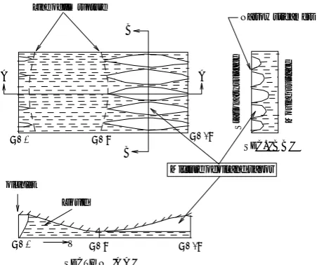
5. CAVITATIONAL MODEL
During iterative solution, whenever the pressure falls below the oil vapor pressure at a grid point, the entire section of the flow, (ξ=ξi), passing
determined at each iteration. A schematic outline of the cavitated region with the film rupture and reformation boundaries is shown in Figure 4. In the cavitated region, based on the experimental observation by Heshmat [16], there are two different parts; 1) narrow oil streamlets extending over the gap and between the film rupture and reformation boundary, and 2) a layer of lubricant adhering to the journal and moving uniformly with the journal speed. The physical model chosen for the analysis is shown in Figure 5. Such detached pattern suggests that there is a very weak bond between the moving streamlets and the stationary surface, permitting side entrainment of gas to take place in the cavitated region.
Since, the range of cavitated domain can be distinguished with the values of lubricant pressure; it is needed to solve the governing equations for obtaining the lubricant pressure in the whole domain. Therefore, in the applied cavitation model, to solve the governing equations which are written for a single phase fluid, an attempt is made to substitute an equivalent fluid in the cavitated region. To formulate this model, it is assumed that a homogenous mixture of lubricant and vapor exists in the cavitated zone with mean physical properties depending on the fraction of liquid and vapor. The liquid fraction, γ, is computed on the basis of continuity requirements. This parameter is defined as the volume of liquid to the total lubricant volume, such that one can compute the density of mixture in the cavitated region by
l
γρ
v
γ)ρ
(1
ρ= − + (26)
The value of γ varies in circumferential direction, such that γ = 1 for the uncavitated part. Now, other mean properties of the mixture such as viscosity and thermal conductivity can be calculated as [8]:
) m
v m 1 ( 1
m ) mv m ( m
l l l
− γ −
= (27)
For computing the value of γ on the basis of continuity requirements, a two-dimensional continuity equation is applied. To reach this goal, and by referring to Figures 4 and 5, if h(θ) and
) (
hl θ are the total film thickness and the liquid film thickness, respectively, then the lubricant mass flow rate with the assumption of uniform velocity distribution for the liquid layer and linear one for the vapor flow is computed as follows:
)] ( h ) ( h [ 2 V v ) ( h V
mθ=ρ θ +ρ θ − θ
l l
l
& (28)
Which, it leads to the following equation for
rs ri
θ, a section in the cavitated region
rupture boundary θ = θ1,
θ = θ2, reformation
boundary
ξ = 0
)θ
ω
Load ψ e
pressure zone ξ = π
Figure 4. The film rupture and reformation boundaries of cavitated region.
Mixture of oil and vapor
M
o
vin
g
su
rfa
c
e
S
tat
io
n
a
ry
s
u
rf
ac
e
Line of film rupture
oil inlet
θ = π
θ = 0 θ = 2π
θ = 0 θ = π θ = 2π
Narrow streamers
V Liquid
B
B
A A
SECTION 'A A '
SEC. ' B B '
computing the liquid film thickness v V 5 . 0 V ) ( h v V 5 . 0 m ) ( h ρ − ρ θ ρ − θ = θ l &
l (29)
Where m&θ is a known parameter which can be computed in the uncavitated region by
∫ θ Δ − θ θ Δ − θ θ ρ = θ i r ) 1 ( dr ) r , 1 ( V m l l
& . (30)
After computing the value of the liquid film thickness from Equation 29, the liquid fraction in the cavitated part of the lubricant flow can be calculated by: )] ( h ) ( h [ 5 . 0 ) ( h ) ( h )] ( h ) ( h [ V 5 . 0 V ) ( h V ) ( h Rate Flow Volume Lubricant Rate Flow Volume Liquid θ − θ + θ θ = θ − θ + θ θ = = γ l l l l l
l (31)
Consequently, according to this model, mean properties of the mixture in the cavitated zone are computed by Equation 27 and all of the governing equations including continuity, momentum and energy equations are solved in the entire flow domain at each iteration. Since, numerical solution of the momentum equation resulted in a negative absolute pressure in the cavitated region; the lubricant pressure was set equal to the vapor pressure for all of the grid points in the cavitated zone. The lubricant vapor pressure in the range of normal oil temperature in the journal bearings is very near to the absolute zero which is considered in the present computations.
It should be mentioned that the details of the applied cavitation model with introducing another two different models are given in the previous paper by the authors [17].
6. SOLUTION PROCEDURE
Finite difference forms of the partial differential
equations were obtained by integrating over an elemental cell volume, with staggered control volumes for the ξ-and η-velocity components. Other variables of interest were computed at the grid nodes. The discretized forms of the governing equations were numerically solved by the SIMPLE algorithm of Patankar, et al [18]. Numerical solutions were obtained iteratively by the line-by-line method.
Numerical calculations were performed by writing a computer program in FORTRAN. As the result of grid tests for obtaining the grid-independent solutions, an optimum grid of 150 × 50 in ξ-and η-directions, with clustering near the journal surface, was used for the flow field calculations and a uniform grid of the same size was considered for the bearing. The main events of the solution process are summarized as follows: 1. A first approximation for each variables U,
V, P, k, ε, T and TB is assumed.
2. The journal surface temperature is obtained as follows:
The first and second approximations of
T
s, at each iteration, are calculated from:∫ ξ η
∫ = s η 0 dξ d ) η , T( π 2
0 sη 1 π 2 1 ) 1 ( s
T (32)
∫ ξ η ξ = 2π
0 d ) s , ( T π 2 1 ) 2 ( s
T (33)
Then, based on having the zero net heat flux for journal surface, the subsequent values of
T
scan be calculated as: ) 1 I ( s q ) 2 I ( s q ) 2 I ( s T ) 1 I ( s T ) 2 I ( s q ) 2 I ( s T ) I ( s T − − − − − − − + − = (34)Where, I is the level of iteration in calculating journal surface temperature.
3. Using Equation 15, lubricant viscosity is computed.
4. U and V velocity components are calculated. 5. Pressure is calculated. When the cavitation
6. Kinetic energy of turbulence and its dissipation rate are calculated.
7. Lubricant temperature, T, is calculated. 8. ∂T/∂n at r = ri is computed.
9. Using the quantity obtained in step 7 for r = ri, TB is calculated.
10. Steps 2 to 9 are repeated until a convergence is achieved.
7. VALIDATION OF COMPUTATIONAL RESULTS
In order to validate the computational results, a test case was analyzed and the result is compared with the experimental data of Reference [19]. Figure 6 shows the pressure distribution around the shaft surface. It can be seen that the pressure increases as the fluid passes through the converging region and remains constant in the cavitated zone. However, the agreement between theoretical and experimental results is satisfactory.
To examine the validation of temperature calculation in the present analysis, in another test case for the Ferron’s bearing [20], the bush inner surface temperature distribution is determined and compared with that in the experiment in Figure 7. The circumferential temperature variations shown in this figure exhibit a similar pattern for both theory and experiment; the temperature rises from the inlet groove to a maximum value approximately near the minimum film thickness, after which the temperature trends to drop. In particular, the value of maximum temperature and its predicted location are reasonably closed to the measurements and the general agreement of the present results with the experimental data is quite good.
8. RESULTS AND DISCUSSIONS
In the present work, the THD characteristic of journal bearings under turbulent flow was examined by CFD technique. It was noted that in the bearings running under lubrication conditions, the clearance ratio was very small in the order of 10-3. However, to show a typical flow field in the
physical domain, numerical solution of the governing equations for the fluid flow between two
eccentric cylinders with large clearance ratio, c/rs =
1, (out of lubrication condition) was obtained. Figure 8 shows the velocity field with drawing the velocity vectors. There are different shapes of velocity profiles at different circumferential sections. This figure indicates a separated flow in the vicinity of maximum film thickness due to the existence of
0 0.2 0.4 0.6 0.8 1
0 π 2π
θ
θ ω
Present work
Expt. (Pan et al. 1976)
P*
Figure 6. Pressure distribution around the shaft surface:, e/c =
0.68, Re = 815 ,c/rs=0.01.
40 45 50 55
θ
0 π 2π
TEM
PER
A
T
U
R
E
(
o C)
θ
Present work
(
54o
ω
Expt.(Ferron et al. 1983)
Figure 7. Bush inner surface temperature Distribution:
50 Re , 0.58 e/c 0.003,
an unfavorable pressure gradient in this region. The present result is in agreement with the numerical and experimental results reported by several other investigators [10].
The variation of turbulent kinetic energy is presented in Figure 9. The value of this parameter may show the amount of flow turbulency in the region of lubricant flow. Figure 9 shows small values for turbulent kinetic energy near the solid boundaries, such that the value of this variable increases in locations far from the boundaries. In the region with unfavorable pressure gradient, there exists a very large turbulent kinetic energy and the maximum value of this parameter occurs in the recirculated zone.
The following results are about an infinite length journal bearing as a test case, in which the
numerical procedure discussed in Section 6 are carried out to obtain THD characteristics of the lubricant flow in turbulent condition. The bearing has an axial groove located on the line of centers at the section of maximum gap, Figure 2a, whose parameters are given in Table 2. The value of Reynolds number Re = 5000 and Peclet number Pe = 14 × 105 are calculated with the clearance ratio
of 0.005. Integration of lubricant pressure over the journal surface provides the value of bearing load.
Figure 8. Velocity vectors: c/rs = 1, e/c = 0.5, Re = 8000.
1.8220E-03 1.6713E-03 1.5206E-03 1.3700E-03 1.2193E-03 1.1188E-03 9.6812E-04 9.4212E-04 9.3226E-04 9.2524E-04 8.9029E-04 8.1744E-04 7.6721E-04 7.1698E-04 6.8192E-04 6.6048E-04 5.1606E-04 3.6538E-04 2.1469E-04 6.4001E-05
Figure 9. Variation of turbulent kinetic energy: c/rs = 1, e/c =
0.5, Re = 8000.
TABLE 2. Bearing Parameters and Lubricant Properties Used In the Test Case.
Parameterer Units Value
rs m 0.05
ri m 0.05005
ro m 0.09
ε — 0.3
θi deg. 7.2
N r.p.m. 271430
w kN/m 392.10
Ti ˚C 40.0
Pi kPa 100.0
Ta ˚C 22.0
μl at 40˚C N.s/m2 0.0192
β 1/˚C 0.032
l
ρ kg/m3 860.0
c
pl J/kg˚C 1970.0
l
K w/m˚C 0.135
B
K w/m˚C 50.0
The following additional property ratios are also needed for the present computations:
1 10 5 p /C v p C , 2 10 17 /K v K
3 10 1.1 /μ v μ , 3 10 1.4 /ρ v ρ
− × = −
× =
− × = −
× =
l l
l l
Pressure distribution around the shaft surface is shown in Figure 10. It is seen that the pressure increases as the fluid passes through the converging zone, such that the maximum value of lubricant pressure occurs at a section before the minimum film thickness. Additionally, this figure shows the extension of cavitated region in which the magnitude of pressure is constant and is equal to the lubricant vapor pressure. It should be noted that in Figure 10, the lubricant pressure is non-dimensionalized by the dynamic pressure ρV2. Figure 11 shows the bush inner surface temperature distribution in the circumferential direction. It can be seen that the value of lubricant temperature increases as the flow passes through the converging region as a result of viscous dissipation. The maximum temperature occurs almost at the section of minimum film thickness after which temperature decreases in the cavitated region. It should be noted that the sharp temperature decrease in the cavitated part of flow is due to the substitution of equivalent fluid in that region, which causes a rapid decrease in the viscous dissipation.
For further investigation of the thermal behavior of journal bearings, isotherms in the bush region are plotted in Figure 12. It is noted that on the metal surface, the maximum temperature is located near the position of minimum film thickness and the minimum temperature, near the oil groove. The heat, which flows normally to the isotherms, is observed to be conducted in the bush and dissipated to the surrounding
9. CONCLUSIONS
In the present work, two dimensional THD analysis based on CFD techniques, has been developed and applied to infinite length journal bearings with turbulent flow. The AKN Low-Re k-ε turbulence model is used to calculate the turbulent stresses and heat fluxes. In the numerical solution of the exact
0 0 .0 5 0 .1 0 .1 5 0 .2
0 π 2π
ω
θ
P
re
ssure
θ
Figure 10. Pressure distribution around the shaft surface.
5 0 1 0 0 1 5 0
θ ω
0 π 2π
θ
T
E
MP
E
R
A
T
URE
(
o C)
Figure 11. Bush inner surface temperature distribution.
A
B
C
D
E F
A B C D E F 50.71 61.88 72.91 83.99 100.61 111.23
governing equations, to avoid any approximation, conformal mapping is used to transfer the physical domain into the computational plane. Finite difference forms of transformed equations are obtained by the control volume method and solved by the SIMPLE algorithm.
The conclusions which may be drawn from this work are summarized as follow:
1. The applied turbulence and cavitation models predict well the pressure, velocity and temperature fields of lubricant flow in both the cavitated and uncavitated parts of journal bearings.
2. The pressure of the lubricant flow increases as it passes through the converging zone and the maximum value of lubricant pressure occurs at a section before the minimum film thickness.
3. As a result of viscous dissipation, lubricant temperature increases as the flow passes through the converging region and the maximum temperature takes place in the vicinity of minimum film thickness, after which the lubricant temperature decreases.
10. NOMENCLATURE
c Radial clearance
cp Specific heat
e Eccentricity h Film thickness
hB Convection heat transfer coefficient
J Jacobian of transformation
k Turbulent kinetic energy K Lubricant thermal conductivity KB Bush thermal conductivity
n Normal direction
P Pressure
rs Shaft radius
ri Inner radius of the bush
ro Bush outer radius
Re Reynolds number
T Lubricant temperature
Ti Inlet lubricant temperature
TB Bush temperature
Ta Ambient temperature
TR Taylor number
(u,v) Velocity components in x-and y-direction
V Linear velocity of the shaft
W bearing load
(x,y) Coordinates in physical domain
Z Physical plane
Greek Letters
α Lubricant thermal diffusivity
β Temperature-viscosity coefficient
γ
Liquid fraction(ε, η) Coordinates in computational domain
μ Lubricant viscosity
μt Turbulent viscosity ρ Lubricant density
θ Angle in the direction of rotation
i
θ
Half angle of groove spanω Angular velocity of the shaft
φ Dissipation
ε Turbulent dissipation rate
Subscripts
a Ambient B Bush
l Lubricant
s Shaft v Vapor
11. APPENDIX
The transformation function ζ = (ari-z)/(az-ri) maps
the circle of radius ri into the unit circle │ζ│ = 1,
while the circle of radius rs is mapped into a circle
of radius Rs in the ζ-plane, Figure 2, where
2 1 ] ) ir a e (
a ir
a e [ s R
− −
= (A1)
and
2 1 ] 1 2 ) i er 2
2 s r 2 e 2 ir ( [ i er 2
2 s r 2 e 2 ir
a= + − − + − − (A2)
region between two concentric circles in the ζ -plane into a rectangle in the λ-plane, with ξ
changing from 0 to 2π and η from 0 to–ln(Rs).
Combining the above transformations gives:
ξ η − + η − +
η − + + ξ +
η − =
cos ae 2 2 e 2 a 1
) 2 e 1 ( a cos ) 2 a 1 ( e fluid ) ir / x
( (A3)
ξ η − + η − +
ξ − η − =
cos ae 2 2 e 2 a 1
sin ) 2 a 1 ( e fluid ) ir / y
( (A4)
From which the metric coefficients xξ, yξ, etc. in
the flow field can be calculated.
For mapping the bush, it is required to have continuous constant θ-lines across the flow field and the bearing in the physical plane. To fulfill this requirement, the function ξ' + iη = -ln(Z/r
i) is used
to map the bearing into a rectangle in the λ-plane, where
⎪⎩ ⎪ ⎨ ⎧
π = ξ π = ξ
= ξ = ξ
+ ξ +
ξ −
− = ξ
for '
0 for 0 '
] a 2 cos ) 2 a 1 (
sin ) 2 a 1 ( [ 1 tan '
(A5)
and (x/ri) and (y/ri) in the bearing are given as:
' cos e ) ir / x
( = −η ξ (A6)
' sin e ) ir / y
( = −η ξ (A7)
From which the metric coefficients in the bearing can be calculated.
12. REFERENCES
1. Frene, J. and Godet, M., “Flow Transition Criteria in a
Journal Bearing”, Trans. of ASME, Journal of
Lubrication Technology, (1974), 135-140.
2. Wilcock, D.F., “Turbulence in High Speed Journal
Bearings”, Trans. ASME, Vol. 72, (1950), 825-834.
3. Constantinescu, V.N., “On Turbulent Lubricant”,
Proc. Inst. Mech. Engrs., Vol. 173, No. 3B, (1959),
881-900.
4. Nagaraju, Y., Joy, M. L. and Prabhakaran Nair, K.,
“Thermohydrodynamic Analysis of A Two-Lobe Journal Bearing”, Int. J. Mech. Sci., Vol. 36, No. 3, (1994),
209-217.
5. Rahimi, A.B., “ Pressure Calculation in the Flow Between Two Rotating Eccentric Cylinders at High Reynolds Numbers”, International Journal of Engineering,
Vol. 9, No. 4, (1996), 201-209.
6. Chun, S.M., “Thermohydrodynamic Lubrication
Analysis of High-Speed Journal Bearing Considering Variable Density and Variable Specific Heat”, Tribology
International, Vol. 37, (2004), 405-413.
7. Peng, Z.C. and Khonsari, M.M., “A Thermohydrodynamic
Analysis of Foil Journal Bearings”, Trans. of ASME,
Journal of Tribology, Vol. 128, (2006), 534-541.
8. Tucker, P.G. and Keogh, P.S., “A Generalized CFD
Approach for Journal Bearing Performance Prediction”,
Proc. Instn Mechanical Engineers, Journal of
Tribology, Vol. 209, (1995), 99-109.
9. Tucker, P. G. and Keogh, P. S., “On the Dynamic
Thermal State in a Hydrodynamic Bearing with a
Whirling Journal using CFD Techniques”, ASME
Journal of Tribology, Vol. 118, (1996), 356-363.
10. Gandjalikhan Nassab, S.A. and Moayeri, M.S., “Three-Dimensional Thermohydrodynamic Analysis of Axially Grooved Journal Bearings”, Proc. Instn. Mech.
Engrs., J. Engineering Tribology, Vol. 216, (2002),
35-47.
11. Gandjalikhan Nassab, S.A., “Inertia Effect on the Thermohydrodynamic Characteristics of Journal Bearings”, Proc. Instn. Mech. Engrs., J. Engineering
Tribology, Vol. 219, (2005), 459-467.
12. Abe, K., Kondoh, T. and Nagao, Y., “A New Turbulence Model for Predicting Fluid Flow and Heat Transfer in Separating and Reattaching Flows-1. Flow Field Calculation”, Int. J. Heat Mass Transfer, Vol. 37, No. 1, (1994), 139-151.
13. Nagano, Y. and Tagawa, M., “An Improvement of the k-ε Turbulence Model for Boundary Layer Flows”, J.
Fluid Engineering, Vol. 112, (1990), 33-39.
14. Dowson, D., Hudson, J., Hunter, B. and March, C. N., “An Experimental Investigation of the Thermal Equilibrium of Steadily Loaded Journal Bearings”, Proc. Inst. Mech.
Engrs., Vol. 131, (1967), 70-80.
15. Gandjalikhan Nassab, S.A., “Analysis of Thermohydrodynamic Characteristics of Journal Bearings”, Ph.D Thesis, University of Shiraz, Shiraz, Iran, (1999).
16. Heshmat, H., “The Mechanism of Cavitation in Hydrodynamic Lubrication”, Tribol. Trans., Vol. 34,
(1991), 177-186.
17. Gandjalikhan Nassab, S.A. and Maneshian, B., “Thermohydrodynamic Analysis of Cavitating Journal Bearings using Three Different Cavitation Models”,
Proc. Instn. Mech. Engrs., J. Engineering Tribology,
Vol. 221, No. 4, (2007), 501-513.
18. Patankar, S.V. and Spalding, B.D., “A Calculation Procedure for Heat, Mass and Momentum Transfer in
Three-Dimensional Parabolic Flows”, International
Journal of Heat and Mass Transfer, Vol. 15, (1972),
1787-1806.
Bearings and Seals”, Bearing and Seals Design in
Nuclear Power Machinery, ASME, (1967),
219-245.
20. Ferron, J., Frene, J. and Boncompain, R., “A Study of
the Thermohydrodynamic Performance of a Plane Journal Bearing; Comparison between Theory and Experiments”, Trans. ASME, J. Lub. Technology, Vol.