Numerical Study of Flow and Heat Transfer in a Square Driven Cavity

(1)

NUMERICAL STUDY OF FLOW AND HEAT TRANSFER

IN A SQUARE DRIVEN CAVITY

H. Shokouhmand and H. Sayehvand

Department of Mechanical Engineering, Tehran University Tehran, Iran, [email protected] - [email protected]

(Received: February 13, 2004 - Accepted in Revised Form: May 10, 2004)

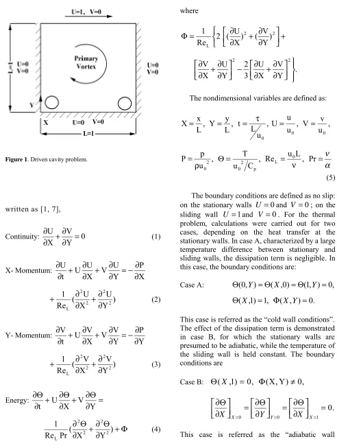
Abstract A numerical approach called “SIMPLER” is used to investigate the flow and heat transfer characteristics in a square driven cavity. The two-dimensional incompressible Navier-Stokes equations were solved and the results are depicted as contour plots of stream function, vorticity, and total pressure for Reynolds numbers from 1 to 10000. At the higher values of Reynolds number, an inviscid core region develops, but secondary eddies are present in the bottom corners of the square at all Reynolds numbers. In addition, the energy equation was solved and isotherms and wall heat-flux distributions are graphically presented. The finding of the present numerical solutions with those given in the literature is in good agreement.

Key Words SIMPLER, Square cavity, Reynolds, Viscous region, Vorticity

ﻩﺪﻴﻜﭼ

ﻡﺎﻧﻪﺑ ﻱﺩﺪﻋﺵﻭﺭﻚﻳ ﺯﺍ

”

ﺮﻠﭙﻤﻴﺳ

”

ﻩﺭﺍﻮﻳﺩﻩﺮﻔﺣﺭﺩﺕﺭﺍﺮﺣ ﻝﺎﻘﺘﻧﺍﻭﻥﺎﻳﺮﺟ ﻲﺳﺭﺮﺑﻱﺍﺮﺑ

ﻙﺮﺤﺘﻣ

ﺖﺳﺍ ﻩﺪﺷ ﻩﺩﺎﻔﺘﺳﺍ ﻞﻜﺷﻲﻌﺑﺮﻣ

.

ﺮﻳﻭﺎﻧﺮﻳﺬﭘﺎﻧﻢﻛﺍﺮﺗ ﻱﺪﻌﺑﻭﺩ ﺕﻻﺩﺎﻌﻣ

ﺞﻳﺎﺘﻧﻪﻛ ﻩﺪﻳﺩﺮﮔﻞﺣ ﺲﻛﻮﺘﺳﺍ ﻱﺍﺮﺑ

ﺯﺍﺯﺪﻟﻮﻨﻳﺭﺩﺍﺪﻋﺍ

١ ﺎﺗ ١٠٠٠٠

ﻢﻫﻱﺎﻫﻲﻨﺤﻨﻣﺕﺭﻮﺻﻪﺑ

ﺪﻧﺍﻩﺪﺷﻩﺩﺍﺩﻥﺎﺸﻧﻞﻛﺭﺎﺸﻓﻭﺶﺧﺮﭼ،ﻥﺎﻳﺮﺟﻂﺧﺯﺍﺮﺗ

.

ﺭﺩﺪﻨﻫﺩﻲﻣﻥﺎﺸﻧﺞﻳﺎﺘﻧ

ﺮﻳﺩﺎﻘﻣ ﺮﺗﻻﺎﺑ ﺩﺪﻋ ﺯﺪﻟﻮﻨﻳﺭ

،

ﻚﻳ ﻪﺘﺴﻫ

ﺝﺰﻟﺮﻴﻏ

ﺩﺎﺠﻳﺍ

ﺩﺩﺮﮔﻲﻣ

.

ﺭﺩﻪﻳﻮﻧﺎﺛﻱﺎﻫﻪﺑﺍﺩﺮﮔﻲﻟﻭ

ﻱﺎﻫﻪﺷﻮﮔ

ﺭﺩﻲﻨﻴﻳﺎﭘ

ﺩﺍﺪﻋﺍﻡﺎﻤﺗ

ﺯﺪﻟﻮﻨﻳﺭ

ﻲﻣﻩﺪﻫﺎﺸﻣ

ﺪﻧﻮﺷ

.

ﻱﺎﻫﻲﻨﺤﻨﻣ ﻪﻛ ﻩﺪﻳﺩﺮﮔﻞﺣﻱﮊﺮﻧﺍﻪﻟﺩﺎﻌﻣﻩﻭﻼﻋ ﻪﺑ

ﻢﻫ

ﻪﺑﻲﺗﺭﺍﺮﺣﺭﺎﺷ ﻊﻳﺯﻮﺗﻭﺎﻣﺩ

ﺪﻧﺍﻩﺪﺷﻩﺩﺍﺩﺶﻳﺎﻤﻧﻲﻜﻴﻓﺍﺮﮔﺕﺭﻮﺻ

. ﺎﺑﻪﺘﻓﺭﺭﺎﻜﺑﻱﺩﺪﻋﺵﻭﺭﺞﻳﺎﺘﻧﻪﺴﻳﺎﻘﻣ

ﺮﮕﻳﺩﻱﺎﻫﺵﻭﺭﺞﻳﺎﺘﻧ

ﺍﺭﻲﺑﻮﺧﻖﻓﺍﻮﺗ

ﻥﺎﺸﻧ

ﺪﻫﺩﻲﻣ

.

1. INTRODUCTION

W a l l b o u n d a r i e s s u r r o u n d i n g t h e e n t i r e computational region in the driven cavity problem is a classic problem. In this problem, the incompressible viscous flow in the cavity is driven by the uniform translation of the upper surface (lid). The driven cavity problem is an excellent test case for comparing methods that solve the incompressible Navier-Stokes equations. Detailed computational results for the driven cavity problem can be found in Burggraf [1], Bozeman and Dalton [2], Rubin and Harris [3] and Ghia et al [4], while

experimental data is available in Mills [5] and Pan and Acrivos [6].

In the present treatise, the driven flow in a

square cavity was used as the model problem. Numerical solutions were obtained for configurations with Reynolds number as high as 10,000, using the SIMPLER method and were compared with solutions available in the literature.

2. MATHEMATICAL FORMULATION

The cavity flow geometry and coordinates

)

,

(2)

written as [1, 7],

Continuity:

0

Y

V

X

U

=

∂

+

∂

(1) X- Momentum:

X

P

Y

U

V

X

U

t

U

∂

−

=

∂

+

∂

+

∂

)

Y

U

X

U

(

Re

1

2 2 2 2 L

∂

+

∂

+

(2)

Y- Momentum:

Y

P

Y

V

X

V

U

t

V

∂

−

=

∂

+

∂

+

∂

)

Y

V

X

V

(

Re

1

2 2 2 2 L

∂

+

∂

+

(3)

Energy:

=

∂

Θ

∂

+

∂

Θ

∂

+

∂

Θ

∂

Y

V

X

U

t

+

Φ

∂

Θ

∂

+

∂

Θ

∂

)

Y

X

(

Pr

Re

1

2 2 2 2 L (4) where







+









∂

+

∂

=

Φ

2 2

L

)

Y

V

(

)

X

U

(

2

Re

1

.

Y

V

X

U

3

2

Y

U

X

V

2 2

















∂

+

∂

−









∂

+

∂

The nondimensional variables are defined as:

,

L

x

X

=

,

L

y

Y

=

,

u

L

t

0

τ

=

,

u

U

0

=

,

u

v

V

0

=

,

u

p

P

₂ 0

ρ

=

,

C

u

T

p 2 0

=

Θ

Re

u

0

L

,

L

=

ν

α

ν

=

Pr

(5) The boundary conditions are defined as no slip:

on the stationary walls U =0and V =0; on the

sliding wall U =1and V =0. For the thermal

problem, calculations were carried out for two cases, depending on the heat transfer at the stationary walls. In case A, characterized by a large temperature difference between stationary and sliding walls, the dissipation term is negligible. In this case, the boundary conditions are:

Case A:

Θ

(

0

,

Y

)

=

Θ

(

X

,

0

)

=

Θ

(

1

,

Y

)

=

0

,

1

)

1

,

(

=

Θ

X

Φ

(

X

,

Y

)

=

0

.

This case is referred as the “cold wall conditions”. The effect of the dissipation term is demonstrated in case B, for which the stationary walls are presumed to be adiabatic, while the temperature of the sliding wall is held constant. The boundary conditions are

Case B:

Θ

(

X

,

1

)

=

0

,

Φ

(

X

,

Y

)

≠

0

,

.

0

1 0 0

=









∂

Θ

∂

=









∂

Θ

∂

=









∂

Θ

∂

= =

= Y X

X

Y

X

This case is referred as the “adiabatic wall

(3)

condition”. In both cases, the Prandtl number was taken as unity for convenience [1].

3. NUMERICAL SCHEME

In order to solve the above system of equations, the well-established SIMPLER numerical solution technique of Patankar [8] was employed. A combination of line-by-line and block-correction methods was used to solve the resulting algebraic equations [9 and 10]. Typically, 15000 iterations were required to achieve convergence, which took 15-20 minutes of computational time on a Pentium-II processor and this increased drastically by mesh refinement. For each grid point, a residual

R can be calculated from the resulting discretization equation as:

∑

φ

+

−

φ

=

a

b

a

,

R

_nb _nb _P _P (6)

where

∑

a_nbφ_nbshows all neighbor terms. The

convergence criterion adopted was that R for

each grid point, between two successive iterations were smaller than a pre-assigned value of 10−4. The spatial grid was typically 57×57 in the

Y

X− computational domain. The sensitivity of calculated results to the grid interval, time step, and convergence criterion was checked in several sample calculations. The computational parameters that were selected for the present work were found

(4)

to yield satisfactory results in the grid- and time step-convergence tests.

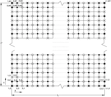
The staggered computational grid that is shown in Figure 2 was used. There are three systems of grid points shown in Figure 2; the solid points are where

P

is calculated, the open points are where

Uis calculated, and the points denoted by

×

are where Vis calculated. The use of a staggered grid requires careful attention to the indexing system that identifies each set of points, which somewhat complicates the coding of the computer program. There are various ways of setting up the logic dealing with the proper bookkeeping for a staggered grid. In Figure 2, each set of points has its own independent indexing. For example, the “

P

points” run from 1 to

L

₁ in the

X

direction and from 1 to

M

₁ in the

Y

direction, the “U

L

₁ in the

X

M

₁ in the

Y

direction, and the “V

L

₁ in the

X

M

₁ in the

Y

direction.

4. RESULTS AND DISCUSSION

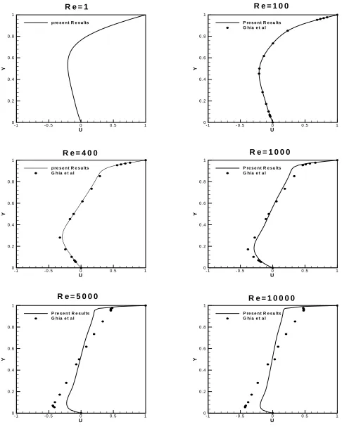
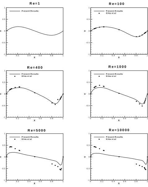
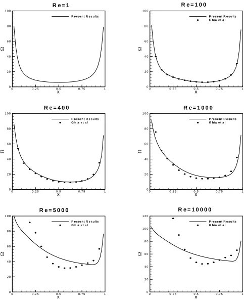
To verify the computer code, results of the SIMPLER method have been compared with those reported in [4]. U-velocity along vertical line and V-velocity along horizontal line through geometric centre of the cavity are shown in Figures 3 and 4 respectively. Figure 5 shows vorticity on the moving wall.

It is seen that the results obtained in the present work are in good agreement with those reported in [4] at all Reynolds numbers, especially at the lower ones. This indicates the validity of the numerical code that has been developed. It should be pointed out that the numerical results of [4] were obtained on a finer mesh of 129×129 grid nodes that can be the most likely reason for the differences seen at the higher Reynolds numbers.

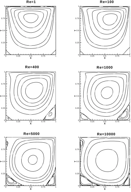
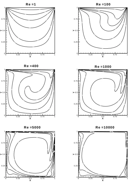
The development of the flow with Reynolds number is shown in Figures 6 and 7 at different conditions. The streamline pattern is only slightly affected by Reynolds number; however, the shift of vortex centre with increasing Re is clearly evident, first in the downstream direction (of the

moving boundary) and then toward the centre of the square.

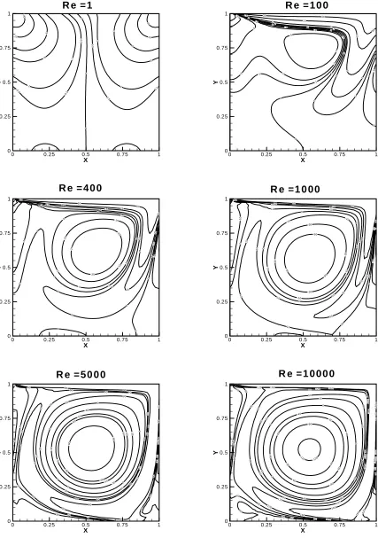
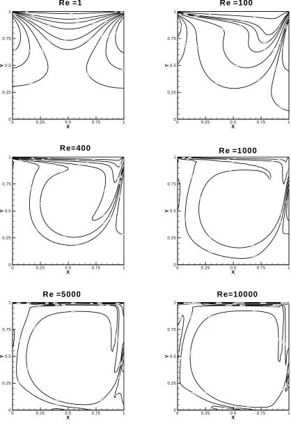
The vorticity distribution (Figure 7) provides a stronger measure of the effect of viscosity. The symmetric pattern at low Reynolds numbers is due to the vanishing of the convection effects. However, at higher Reynolds numbers, these effects would eventually dominate the flow, producing a core of nearly uniform vorticity. Note the strong variation of vorticity in the boundary layer, especially along the top and the right side of the cavity. The interaction of convection and viscous diffusion of vorticity in the viscous annulus is indicated by the “stretching” of the contours in the direction of the flow.

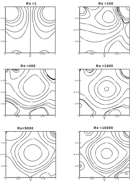
The non-dimensional total pressure is:

pT L 0

B T

T Re C

2 1 u

L ) p p (

P =

µ − =

with reference to the pressure

p

_B at the centre of

the bottom wall of the cavity. The static and total pressure contours are shown in Figures 8 and 9. In the completely viscous limit, the static and total pressure become identical and shows no resemblance to the streamlines. Since the pressure is then a harmonic function, the contours cannot be closed but must end on the boundaries. Conversely, for the inviscid limit, total pressure is conserved on streamlines, so that the contours of total pressure would be identical to the streamlines. This development from fully viscous to inviscid flow is clearly depicted by Figure 9.

At Re = 100, a very small inviscid core has developed around the vortex center, while at Re = 400, the inviscid core has grown to a diameter about 1/3 that of the cavity. From these plots, we conclude that the total pressure distribution is a good measure relating to the degree of viscous and inviscid flow. The interaction of convection and viscous diffusion of total pressure along the streamlines is indicated just as for vorticity. Actually, in steady flow, the total pressure obeys a diffusion equation with a “source” term representing a viscous loss proportional to the square of the vorticity.

. P

Re 1 Dt

DP 2

T 2

L

(5)

U

Y

-1 -0 .5 0 0 .5 1

0 0 .2 0 .4 0 .6 0 .8 1

p re s e n t R e su lts R e = 1

U

Y

-1 -0 .5 0 0 .5 1

0 0 .2 0 .4 0 .6 0 .8 1

P re s e n t R e su lts G h ia e t a l

R e = 1 0 0

U

Y

-1 -0 .5 0 0 .5 1

0 0 .2 0 .4 0 .6 0 .8 1

p re s e n t R e su lts G h ia e t a l

R e = 4 0 0

U

Y

-1 -0 .5 0 0 .5 1

0 0 .2 0 .4 0 .6 0 .8 1

R e = 1 0 0 0

U

Y

-1 -0 .5 0 0 .5 1

0 0 .2 0 .4 0 .6 0 .8 1

P re se n t R e s u lts G h ia e t a l

R e = 5 0 0 0

U

Y

-1 -0 .5 0 0 .5 1

0 0 .2 0 .4 0 .6 0 .8 1

R e = 1 0 0 0 0

(6)

X

V

0 0 .2 0 .4 0 .6 0 .8 1

-1 -0 .5 0 0 .5 1

P re s e n t R e s u lts R e = 1

X

V

0 0 .2 0 .4 0 .6 0 .8 1

- 1 - 0 .5 0 0 .5 1

P re s e n t R e s u lts G h ia e t a l

R e = 1 0 0

X

V

0 0 .2 0 .4 0 .6 0 .8 1

-1 -0 .5 0 0 .5 1

R e = 4 0 0

X

V

0 0 .2 0 .4 0 .6 0 .8 1

- 1 - 0 .5 0 0 .5 1

R e = 1 0 0 0

X

V

0 0 .2 0 .4 0 .6 0 .8 1

-1 -0 .5 0 0 .5 1

R e = 5 0 0 0

X

V

0 0 .2 0 .4 0 .6 0 .8 1

- 1 - 0 .5 0 0 .5 1

R e = 1 0 0 0 0

(7)

X

Ω

0 0 .2 5 0 .5 0 .7 5 1

0 2 0 4 0 6 0 8 0 1 0 0

P re s e n t R e s u lts R e = 1

X

Ω

0 0 .2 5 0 .5 0 .7 5 1

0 2 0 4 0 6 0 8 0 1 0 0

P re s e n t R e s u lts G h ia e t a l R e = 1 0 0

X

Ω

0 0 .2 5 0 .5 0 .7 5 1

0 2 0 4 0 6 0 8 0 1 0 0

P re s e n t R e s u lts G h ia e t a l R e = 4 0 0

X

Ω

0 0 .2 5 0 .5 0 .7 5 1

0 2 0 4 0 6 0 8 0 1 0 0

P re s e n t R e s u lts G h ia e t a l R e = 1 0 0 0

X

Ω

0 0 .2 5 0 .5 0 .7 5 1

0 2 0 4 0 6 0 8 0 1 0 0

P re s e n t R e s u lts G h ia e t a l R e = 5 0 0 0

X

Ω

0 0 .2 5 0 .5 0 .7 5 1

0 2 0 4 0 6 0 8 0 1 0 0 1 2 0

P re s e n t R e s u lts G h ia e t a l R e = 1 0 0 0 0

(8)

-0_.09 -0_.0 9 -0.07 _-0.07 -0.07 -0_.0 5 -0.05 -0.05 -0.0 5 -0.05 -0_.0 3 -0.03 -0.03 -0 .03 -0.0 3 -0.03 -0 .01 -0_.0 1 -0.01 -0.01 -0 .01 -0.0 1 -0.01 -0.005 -0_.0 05 -0 .0 0 5 -0.005 -0.005 -0.0 0 5 -0.0 05 -0.005 0 0

0 0 0

0 0 0 0 X Y

0 0.25 0.5 0.75 1

0 0.25 0.5 0.75 1 R e=1

-0.09

-0.0 9 -0_.07 -0.07 -0_.0 7 -0.07 -0 .05 -0.05 -0.05 -0.0 5 -0.05 -0_.0 3 -0.03 -0.03 -0 .0 3 -0.0 3 -0.03 -0.01 -0 .0 1 -0 .0

1 -0.01 -0.01

-0.0 1 -0.0 1 -0.01 -0_.00 5 -0 .0 0 5 -0.0

05 -0.005 -0.005

-0.0 0 5 -0.0 05 -0.005 0 0

0 0 0

0 0 0 0 X Y

0 0.25 0.5 0.75 1

0 0.25 0.5 0.75 1 R e=100 -0.0

9 -0.0

9 -0.0 7 -0.07 -0.0 7 -0.07 -0_.0 5 -0.0 5 -0.05 -0.0 5

-0.05

-0_.0 3 -0.0 3 -0.03 -0 .0 3 -0.0 3 -0.03 -0_.0 1 -0 .0 1

-0.01 -0.01 -0.01

-0.0 1 -0.0 1 -0.01 0 0 0 0 0 0 0 1E -05 0 1E-0 5 1E-05 5E-0 5 5E -05 0.00

0 5

X

Y

0 0.25 0.5 0.75 1

0 0.25 0.5 0.75 1 R e=400 -0 .09 -0.0 9 -0.0 7 -0.07 -0.0 7 -0.07 -0_.0 5 -0.05 -0.05 -0.0 5 -0.05 -0.03 -0 .0 3 -0.03 -0.03 -0 .03 -0.0 3 -0.03 -0.01 -0_.0 1 -0.0 1 -0.01 -0.01 -0.0 1 -0.0 1 -0.01 0 0 0 0 0 0 0 0 0 5E_-05 5E-0 5 5 E -0 5

0.000 5 0.000 5 0.00 1 X Y

0 0.25 0.5 0.75 1

0 0.25 0.5 0.75 1 R e=1000 -0.06 -0.0 6 -0 .05 -0.05 -0.0 5 -0 .03 -0.0 3 -0.03 _-0 .03 -0.0 3 -0.03 -0_.0 2 -0.0 2 -0.02 -0.02 -0 .02 -0.0 2 -0.02 -0 .01 -0.0 1 -0.01 -0.01 -0 .0 1 -0.0 1

-0.01

-0.01 0

0

0 0 0

0

0 0

5E-05

5E-0 5 5 E -0 5 0.0₀₀₅ 0.00 05 0.0005 0_.0 0 1

0.001 0.001

X

Y

0 0.25 0.5 0.75 1

0 0.25 0.5 0.75 1 R e=5000 -0.0 4 -0.04 -0.0 4 -0_.0 2 -0.0 2 -0.02 -0.02 -0 .0 2

-0.02 -0.02 -0.01 -0 .0 1 -0.0 1 -0.01 -0.01 -0 .0 1 -0.0 1 -0.01 -0.001 -0 .0 0 1 -0.0 0 1

-0.001 -0.001 -0.001

-0 0 0 1 -0.0 01 -0.001 0 0

0 0 0

0 0 0 0 0 5E-05 5 E -0 5 5 E-0 5 5E_-05 0.0001 0 .00 0 1 0.000 1 0.0₀₀ 5 0 .0 0 0 5 X Y

0 0.25 0.5 0.75 1

0 0.25 0.5 0.75 1 R e=10000

(9)

-3 -3 -3 -3 -3 -3 -1 -1 -1 -1 -1 -1 -1 -1 -1 -1 -0.5 -0 .5 -0.5 -0 .5 -0.5 -0.5 -0.5 -0.5 0 0 0 0 0 0 0 0 0 0.5 0_.5 0.5 0.5 0.5 0.5 0 .5 0.5 0.5 0.5 0 .5 1 1 1 1 1 1 1 1 1 1 1 1 1 2 2 2 2 2 2 2 3 3 3 3 X Y

0 0.25 0.5 0.75 1

R e= 5 0 0 0

-5 -5 -5 -5 -1 -1 -1 -1 -1 -1 -1 -1 -1 -0.5 -0 .5 -0.5 -0.5 -0.5 -0.5 -0.5 -0 .5 -0 .5 0 0 0 0 0 0 0 0 0 0 0.5 0 .5 0 .5 0.5 0.5 0.5 0.5 0.5 0.5 0.5 0.5 0.5 0 .5 1 1 3 1 1 1 1 1 1 1 1 3 3 3 3 3 3 3 3 X Y

0 0.25 0.5 0.75 1

R e= 1 0 0 0 0 -5 -5 -5 -2 -2 -2 -2 -2 -1 -1 -1 -1 -1 -1 -1 -0.1 -0.1 -0.1 -0 .1 -0.1 -0.1 -0.1 0 0 0 0 0 0 0 0 3 1 1 1 1 1 2 2 2 2 2 2 3 3 3 3 5 5 5 X Y

0 0.25 0.5 0.75 1

R e= 4 0 0

-5 -5 -5 -3 -3 -3 -3 -3 -1 -1 -1 -1 -1 -1 -1

-1 -0.3

-0.3

-0

.3

-0.3 -0.3

-0.3 -0 .3 0 0 0 0 0 0 0 0 1 1 1 1 1 1 1 2 2 2 2 2 2 3 3 3 3 X Y

0 0.25 0.5 0.75 1

R e=1 0 0 0 -3 -3 -1 -1 -0.5 -0_.5 -0_.5 -0.5 -0.1 3 -0 .1 -0.1 -0.1 -0.1 0 0 0 0 0 0 1 1 1 1 3 3 3 5 5 5 X Y

0 0.25 0.5 0.75 1

0 0.25 0.5 0.75 1 R e=1 -3 0_.1 -1 0 -1 -1 -0.5 -0.5 -0_.5 -0.5 -0.5 -0.5 0.1 0 0 0 0 0.1 0 .1 0.1 0.1 0.1 3 3 3 5 5 5 X Y

0 0.25 0.5 0.75 1

R e= 1 0 0

(10)

-0.08 -0_.0 8 -0_.0 8 -0_.0 6 -0 .06

-0.06

-0 .0 6 -0.04 -0.04 -0_.0 4 -0.04 -0.02 -0.02 -0 .02 -0_.0 05 -0.0 05 -0.005 -0.005 -0.0 05 -0 .00 5 0 0 0 0.0025 0_.0 02 5 0 .02 0.04 X Y

0 0.25 0.5 0.75 1

R e = 1 0 0

-0.0 7 -0_.0 7 -0.0 7 -0.0 5 -0_.0 5 -0.0 5 -0.0 5 -0_.0 5 -0.0 3 -0.03 -0_.0 3 -0.0 3 -0_.0 3 -0.01 -0.01 -0.01 -0.0 1 -0.005 -0.0₀₅ -0.005 -0 .005

-0.003 -0.0 03 -0_.0 03 -0 .00 05 -0.0005 0 0 0 5 0 0 0 0 X Y

0 0.25 0.5 0.75 1

R e = 4 0 0

-0.07 -0.0

6 -0.06

-0.06

-0 .05

-0.0

5 -0.05

-0.0 5 -0.0

3 -0.03 -0 .03 -0.0 3 -0.0 -0_.0 3

-0.01

-0_.01 -0_.0 1 0 0 0 0 0 0.0 01 0.001 0.0 01 005 0.005 0.0 05 X Y

0 0.25 0.5 0.75 1

R e = 1 0 0 0

-0.0 2 -0.0 2 -0.0₁₅ -0.0 1 5 -0.015 -0 .01 5

-0.015

-0.0 1 -0_.0 1 -0.01 -0.0 1 -0.01

-0.005 -0.0₀₅

-0_.0 05

-0.005 -0.0 05 0 0 0 0 0 0.01 X Y

0 0.25 0.5 0.75 1

R e= 5 0 0 0

-0.0 12

-0.012

-0_.0 1 -0.01 -0.0 1 -0 .007

-0.0 07 -0_.0 07 -0_.0 0 7

-0.007

-0_.0 07

-0.0 05

-0.005 -0_.0 05 -0.0 05 -0.0 05 -0_.0 05

-0.003

-0.0 03 -0_.0 0 3 -0.0 03 -0.003 0 0 0 0 0 0

0.005

0.0 05 0.00 7 0.0₀₇ 0.01 X Y

0 0.25 0.5 0.75 1

R e = 1 0 0 0 0

-4 -3 -3 -2 -2 -1 -1 -1 -0.5 -0.5 -0_.5 0 0 0 0.5 0 .5 1 1 2 2 3 3 4 X Y

0 0.25 0.5 0.75 1

R e = 1

(11)

-20 -10 -5 -3 -1 -1 -0_.5 -0.5 -0 .5 0 0 0 0.5 0.5 0 .5 1 1 3 3 5 10 20 X Y

0 0.25 0.5 0.75 1

R e = 1

-15 -5 -5 -5 -2 -2 -2 -2 -2 -1 -1 -1 -1 -1 0 0 0 0 0 0 0 1 1 1 1 1 2 2 2 2 5 5 5 15 15 1 5 30 30 30 X Y

0 0.25 0.5 0.75 1

R e = 1 0 0

-2 5 -25 -25 -15 -15 -15 -5 -5 -5 -5 -5 -5 -5 -5 0 0 0 0 0 0 0 0 0 0 5 5 5 5 5 5 5 5 15 15 1 5 15 1 5 25 25 2 5 25 60 60 60 60 X Y

0 0.25 0.5 0.75 1

R e = 4 0 0

-50 -50 -50 -3 0 -30 -30 -30 -10 -1 0 -1 0 -10 -10 -10 -10 -10 0 0 0 0 0 0 0 0 0 10 10 10 10 10 1 0 10 1 0 10 10 1 0 30 30 3 0 30 30 30 3 0 50 50 5 0 50 50 80 80 80 8 0 X Y

0 0.25 0.5 0.75 1

R e =1 0 0 0

-90 -90 -6 0 -60 -60 -60 -50 -50 -50 -50 -3 0 -3 0 -30 -3 0 -30 0 0 0 0 0 0 0 0 30 3 0 3 0 3 0 3 0 30 30 3 0 30 30 50 50 50 50 50 50 5 0 50 50 5 0 50 50 60 60 60 6 0 60 60 60 6 0 60 60 60 60 6 0 90 90 9 0 90 90 90 90 90 9 0 X Y

0 0.25 0.5 0.75 1

R e = 5 0 0 0

-1_{2 0}

-120 -90 -90 -90 -60 -60 -60 -60 -4 0 -40 -40 -40 0 0 0 0 0 0 40 40 4 0 4 0 4 0 40 40 40 40 4 0 40 40 60 6 0 6 0 60 6 0 60 60 60 60 60 60 90 90 9 0 90 9 0 9 0 9 0 9 0 90 90 90 90 90 120 120 120 120 1 2 0 1 2 0 120 120 12 0 1 2 0 1 2 0 160 160 1 6 0 1 60 160

160 16

0 1 6 0 1 6 0 X Y

0 0.25 0.5 0.75 1

R e = 1 0 0 0 0

(12)

Hence, in regions of highly rotational flow, the total pressure “streamers” must be shorter than in those of small vorticity. This effect can be seen by comparing Figures 7 and 9. It is also interesting to note that in the upper corners, the static pressure retains its asymmetric singularities over the entire range of Reynolds number, even though taking on a symmetric distribution in the main body of the flow.

A striking feature of the flow field is the growth of the secondary eddies appearing in the bottom corners of the cavity (Figure 6). These triangular shaped eddies, present at all Reynolds numbers, have a diameter of about 10% that of the cavity at Re = 1. However, at Re = 400, the upstream eddy has grown to about 1/3 the diameter of the cavity, although the downstream eddy is relatively unaffected by Reynolds number.

The structure of the flow in the primary eddy is clearly shown by velocity graphs of Figure 3. Velocity profiles are shown for several values of Reynolds numbers. The trend from the rounded profile for Re = 1 to the flattened profiles at high Reynolds numbers is clear. Note in particular the thinning of the boundary layer with increasing Re and the velocity overshoot near the upper wall at high Reynolds numbers. It seems clear that growing the secondary eddy in the bottom of the square cavity prevent the vortex centre from approaching the geometric centre of the cavity.

The distribution of the thermal energy within the recirculating flow is closely analogous to that of vorticity. Owing to the different boundary conditions, the distributions of temperature and vorticity within the boundary layer must differ, but in the limit Re→∞, both tend to become uniform as the inviscid core develops. Sample solutions are presented in Figures 10 and 11 by means of plotted isotherms for different Reynolds numbers. For Stokes flow, the temperature distribution is symmetrical about the vertical centerline of the cavity, in the same way as the flow field. At Re=400 and higher, the isotherms tend to be convected by the flow, forming a pocket of uniform temperature around the vortex centre. For condition B (adiabatic wall), where the region of nearly uniform temperature is much larger, significant variations occur only near the

downstream corner of the moving wall. It is noteworthy that the bottom and upstream walls have nearly uniform temperatures, and that the maximum temperature occurs near the downstream corner of the moving wall. The temperature profiles on the vertical line through the vortex centre are shown in Figure 12 for different Reynolds numbers, with both cold and adiabatic wall conditions. The constancy of the temperature in the inviscid core, as well as the thin thermal boundary layer on the moving wall is clearly evident.

The distribution of non-dimensional temperature gradient (heat flux) along the wall is of considerable interest. Figure 13 shows the ∂Θ ∂Y on the moving wall for condition A (cold wall). The heat flux is distributed symmetrically for Stokes flow, but at the higher Reynolds numbers, a boundary-layer type of distribution is evident, falling from the singularity at the upstream corner to a minimum value very near the downstream corner. Sufficiently near the corner, conduction dominates the heat-transfer mechanism and the asymptotic temperature distribution is

(

θ π

)

− =

Θ 1 2 , where θ is the angle measured from the moving wall. This behavior is clearly evident in Figure 10.

The heat flux to the stationary wall is presented in Figure 14 as ∂Θ ∂N vs. running length ξ for

(13)

0 .0

5

0.05

0.05 0.05

0_.1 0.1 0.1 0.1 0 .1 0_.3 0.3 0.3 0.5 0.5 0.5 0 .7 0.7 0.7 0.9 0.9 X Y

0 0.25 0.5 0.75 1

R e = 1

0 .1 0_.1 0.1 0.1 0 .1 0 .3 0.3 0.3 0.3 0.5 0 .5 0.5 0.5 0.6 0.6 0_.6 0.6 0 .6 0.7 0.7 0.9 0.9 X Y

0 0.25 0.5 0.75 1

R e =1 0 0

0 .1 0 .1 0.1 0.1 0.1 0 .1 0 .1 0.3 0 .3 0.3 0.3 0.3 0 .3 0.5 0.5 0.5

0.5 0.5

0.5 0.55 0.55 0.55 0 .55 0.55 0.5 5 0.7 0.7 0 .7 0.9 0.9 0.9 X Y

0 0.25 0.5 0.75 1

R e =4 0 0

0 .1 0 .1 0.1 0.1 0 .1 0 .1 0.3 0 .3 0.3 0.3 0.3 0 .3 0.5 0.5 0 .5 0 .5 0.5 0 .5 0.5 0.5 0 .5 0.55 0.55

0.55 0.5

5 0.7 0.7 0.7 0.9 0.9 X Y

0 0.25 0.5 0.75 1

R e = 1 0 0 0

0 .1 0_.1 0.1 0.1 0 .1 0 .1 0 1 0.2 0.2 0_.2 0.2 0.2 0 .2 0 .2 0.3 0 .3 0.3 0.3 0.3 0 .3 0 .3 0.4 0.4 0 .4 0 .4 0.4 0.4 0_.4 0.4 0.4 0.4 0 .4 0.45 0.45 0.45 0 .45

0.45

0 .4 5 0.5 0.5 0 .5 0.5 0 .5 0.7 0.7

1 1 1

X

Y

0 0.25 0.5 0.75 1

R e =5 0 0 0

0 .1 0 .1 0 .1 0.1 0.1 0 .1 0 1 0 .2 0 .2 0.2

0.2 0.2

0 .2 0 .2 0.3 0.3 0_.3 0.3 0.3 0 .3 0 .3 0.5 0.5 0 .5 0 .5

0.70.9 0.70.9

X

Y

0 0.25 0.5 0.75 1

R e = 1 0 00 0

(14)

0.1

0.1 0.1

0.3

0.4

0.5 0.5

0.6

0.65

0.65 0.65

0.72

0_.7 2

0.72

0_.7 2

0.72

0

.8

0.8 0 .8

0.9

0

.9

X

Y

0 0.25 0.5 0.75 1

R e =1

0.3

0.3 0.5

0.5

0.5 0.55

0.55

0.6

0.7

0

.8

0.8 0.

8 0 .8

0.85 0 .85

0.8 5

0

.85

0

.9

0

.9

X

Y

0 0.25 0.5 0.75 1

R e =100

0.2

0.3

0.3 0.4

0.4

0.4 0.5

0.5

0.5 0.5 0.55

0.55

0

.5

5

0.55

0.55 0 .55 0.6

0

.6

0_.6

0.6

0.6 0.6

0.7

0

.7

X

Y

0 0.25 0.5 0.75 1

R e=400

0.2 0.2 _0.2

0.3

0.3 0.4

0.4

0.4 0.4

0.4

0.4 0.45

0

.4

5

0.45

0.4 5 0.5

X

Y

0 0.25 0.5 0.75 1

R e =1000

0.15 0.15

0.16 0.16

0.18 0.2 0.18 0.2 0.18

0.24

0

.2

4

0.24 0.24

0.24

0

.2

5

0.25 0.25

0

.2

5

0.25

0

.2

5

0

.25

0.25 0.25

0.26 0_.2

6

0

.26 0.260.26

0.26

X

Y

0 0.25 0.5 0.75 1

R e =5000

0.120.140.15 0.170.2 0.120.140.15 0.170.2 0.120.140.15

0

.2

2

0.22 0.22

0.22

0.2 3

0.23

0

.23

0.23

0

.2

3

0.23

0.23 0.23

0.23

0.235 0.2₃₅

0.2

3

5

0.23 5

0.235 0.235 _0.235 0.235

0.235

0.24

0

.24 0 .24

0.24

X

Y

0 0.25 0.5 0.75 1

Re=10000

(15)

Y

Θ

0 0 .2 5 0 .5 0 .7 5 1

R e = 1

C a s e A C a s e B

Y

Θ

0 0 .2 5 0 .5 0 .7 5 1

R e = 1 0 0

C a s e A C a s e B

Y

Θ

0 0 .2 5 0 .5 0 .7 5 1

R e = 4 0 0

C a s e A C a s e B

Y

Θ

0 0 .2 5 0 .5 0 .7 5 1

R e = 1 0 0 0

C a s e A

C a s e B

Y

Θ

0 0 .2 5 0 .5 0 .7 5 1

R e = 5 0 0 0

C a s e A

C a s e B

Y

Θ

0 0 .2 5 0 .5 0 .7 5 1

R e = 1 0 0 0 0

C a s e A

C a s e B

(16)

boundary-layer theory would be expected to cover most parts of both sidewalls, and this is verified by the results.

5. CONCLUSION

In the present treatise, viscous incompressible flow and heat transfer in a square driven cavity was examined using the SIMPLER algorithm. It is shown that flow in the cavity at low Reynolds numbers follows a symmetric pattern while at higher Reynolds numbers, a thin boundary layer formed on the walls and an inviscid core region develops. Secondary eddies are present in the bottom corners of the square at all Reynolds numbers. The distribution of thermal energy within the recirculating flow is closely analogous to that of vorticity. Comparison of the results obtained in this work with those reported in the literature showed that SIMPLER is an accurate and reliable method for computation of convective heat transfer problems.

6. ACKNOWLEDGEMENTS

Financial support for this research, provided by the Research Deputy of University of Tehran through Grant 618/2/1070, is greatly appreciated.

7. NOMENCLATURE

a oefficient in discretization equation

b source term in discretization equation P

C

specific heat capacity of fluid

L

cavity width

1

L

last grid point in

X

direction 1

M

last grid point in

Y

direction

N coordinate normal to the surface

p

pressure

P

non-dimensional pressure T

P

non-dimensional total pressure

Pr

Prandtl number

X

HE

A

T

F

L

UX

0 0.2 0.4 0.6 0.8 1 0

20 40 60 80 100 120

Re=1 Re=100 Re=400 Re=1000 Re=5000 Re=10000

Figure 13. Normalized heat flux on moving wall for Case A.

ξ

HE

A

T

F

L

UX

1 2 3 4

10 20 30

Re=1 Re=100 Re=400 Re=1000

(17)

L

Re

Reynolds number

t

non-dimensional time T temperature

U

,

u

velocity 0

u

velocity of moving wall

V

v

,

velocity

X

x

,

coordinates

Y

y

,

coordinates

Greek Symbols

α thermal diffusivity of fluid

Θ non-dimensional temperature

µ

dynamic viscosity

ν

kinematic viscosity

ξ

length

ρ

density

τ

time

φ

general variable

Φ

dissipation function

Subscripts

P

grid point

8. REFERENCES

1. Burggraf, O. R., “Analytical and Numerical Studies of the

Structure of Steady Separated Flows”, J. Fluid Mech., Vol. 24, (1966), 113-151.

2. Bozeman, J. D. and Dalton, C., “Numerical Study of

Viscous Flow in a Cavity”, J. Comp. Phys., Vol. 12,

(1973), 348-363.

3. Rubin, S. G. and Harris, J. E., “Numerical Studies of Incompressible Viscous Flow in Driven Cavity”, NASA, (1975), SP-378.

4. Ghia, U., Ghia, K. N. and Shin, C. T., “High-Re Solution for Incompressible Flow Using the N a v i e r - S t o k e s E q u a t i o n s a n d a M u l t i g r i d

Method”, J. Com p. Phys., Vol. 48, (1982),

387-411.

5. Mills, R. D., “Numerical Solutions of the Viscous Flow

Equations for a Class of Closed Flows”, J. R. Aeronaut.