Please cite this article as: I. Tadayoni Navaei, B. Zafarmand, Random Vortex Method for Geometries with UnsolvableSchwarz-Christoffel Formula, International Journal of Engineering (IJE), IJE TRANSACTIONS A: Basics Vol. 31, No. 1, (January 2018) 38-44
International Journal of Engineering
J o u r n a l H o m e p a g e : w w w . i j e . i rRandom Vortex Method for Geometries with Unsolvable
Schwarz-Christoffel
Formula
I. Tadayoni Navaei*a, B. Zafarmandb
a Department of Mechanical Engineering, Mashhad Branch, Islamic Azad University, Mashhad, Iran bDepartment of Mechanical Engineering, Institute of Energy & Hydro Technology (IEHT), Mashhad, Iran
P A P E R I N F O
Paper history: Received 21 January 2017
Received in revised form 18 September 2017 Accepted 30 November 2017
Keywords: Flow Field
Numerical Simulation Open Cavity
Random Vortex Method Turbulent
A B S T R A C T
In this research we have implemented the Random Vortex Method to calculate velocity fields of fluids inside open cavities in both turbulent and laminar flows. the Random Vortex Method is a CFD method (in both turbulent and laminar fields) which needs the Schwarz-Christoffel transformation formula to map the physical geometry into the upper half plane. In some complex geometries like the flow inside cavity, the Schwarz-Christoffel mapping which transfers the cavity into the upper half plane cannot be achieved easily. In this paper, the mentioned mapping function for a square cavity is obtained numerically. Then, the instantaneous and the average velocity fields are calculated inside the cavity using the RVM. Reynolds numbers for laminar and turbulent flows are 50 and 50000, respectively. In both cases, the velocity distribution of the model is compared with the FLUENT results that the results are very satisfactory. Also, for aspect ratio the cavity (α) equal 2, the same calculation was done for Re=50 and 50000. The advantage of this modelling is that for calculation of velocity at any point of the geometry, there is no need to use meshing in all of the flow field and the velocity in a special point can be obtained directly and with no need to the other points.
doi: 10.5829/ije.2018.31.01a.06
NOMENCLATURE
A Area z physical plane Vectors
F Schwarz-Christoffel transformation function Greek Symbols u Velocity vector
G Green’s function Transformation plane n Unit vector normal to the wall
h Vortex sheets η Gaussian random variable s Unit vector tangential to the wall k Time interval Circulation per unit length
p Pressure σ Standard deviation Re Reynolds number Dirac delta function
r radius Dilatation
RVM Random Vortex Method Gradient operator
t Time Vorticity
V Volume Circulation
W(u,v) Complex Velocity Stream function
1. INTRODUCTION1
Facing the turbulent flows is inevitable in daily life and there is a certain need to study this kind of flows in detail to understand its characteristics [1]. Chorin represented a meshless method to solve the turbulent flows by using the
*Corresponding Author’s Email:[email protected] (I. Tadayoni Navaei)
[6] and further improvements in the analysis were given by Cottet [7]. Vortex method was later incorporated into a hybrid vortex-boundary element algorithm for the simulation of viscous flow inside 3-D geometries with moving boundaries of the type found in engines [8].
Methods which rely on vortex methods have achieved extensive popularity recently and have been utilized in a vast range of settings [3, 9-12]. Some early applications have focused on anticipating gross qualitative types of turbulent flow [13-15] and on comparing their results with experiments [16, 17]. Furthermore, numerical precision of the RVM has been studied by [5] for complex flows in laminar and high Reynolds number turbulent flows. Various researches have been performed in the field. H. Shokouhmand et al. [18] used a numerical method to investigate the flow and heat transfer characteristics in a square driven cavity for Reynolds numbers from 1 to 10000. M. Taghilou et al. [19] used the single relaxation time (SRT) lattice Boltzmann equation to simulate lid driven cavity flow at different Reynolds numbers (100-5000). Their investigation showed that with increasing the Reynolds number, bottom corner vortices will grow but they won’t merge together. In addition, the merger of the bottom corner vortices into a primary vortex and creation of other secondary vortices was shown in the cases which the aspect ratios are bigger than one. B. Zafarmand and coworkers [20] studied turbulent flow in a channel using Vortex Blob Method (VBM) and obtained physical concepts of turbulence. In their work, time-averaged velocities, and then their fluctuations are calculated. M. Taghilou et al. [19] used the SRT lattice Boltzmann equation to simulate lid driven cavity flow at different Reynolds numbers (100-5000) and three aspect ratios, K=1, 1.5 and 4.
The main reason that meshless methods are significantly interested is that the well-established and successful numerical methods like the finite volume/finite elements need a mesh. The automatic generation of a high quality mesh poses a serious problem in the analysis of practical engineering systems. Furthermore, the analysis and simulation of certain types of problems (like dynamic crack propagation) require an expensive remeshing operation. Meshless methods overcome these problems associated with meshing by eliminating the mesh altogether [21].
In this research we obtain the angels of Schwarz-Christoffel transformation mapping with numerical method, then use the mapping in the Random Vortex Method to calculate turbulent and laminar flow field inside square and rectangular open cavities by the Random Vortex Method.
2. NUMERICAL SCHEME
2. 1 Formulation Navier-Stokes and continuity equations, due to the vorticity-most important aspect of turbulence- and vortex stretching effects in the two
dimensional formulation, will be simplified to
1 2
/ Re
Du Dt u p (1)
Here, Re plays the role of Reynolds number at inlet of the system and u=(u,v) signifies the velocity which is normalized, p is the normalized pressure and shows the gradient operator, 2 expresses the Laplacian, and
.
Du u
Dt t
implies the substantial derivative.
By solving these equations considering the boundary conditions, the flow field is specified
at inlet u = (1,0) (2)
On the walls u = 0 (3)
As we know, the second element of the flow field is vorticity
u (4)
Then:
1 2
/ Re
D Dt (5)
u(r) will be achieved by (1) and (4), when (5) is utilized for updating ω(x, y) - the field of velocity.
Based on the Helmholtz’s Theorem [2, 16] the mechanism of momentum transport, is revealed by a synthetic method of approach, velocity decomposition theorem (known also as the Hodge decomposition), that plays a vital role in contemporary computational fluid mechanics. According to Helmholtz’s Theorem, the velocity vector is discretized into a divergence-free, irrotational, rotational and curl-free components i.e.
uu u (6)
where ∇.uω ≡ 0 (7)
while ∇×u∆ ≡ 0 (8)
Both the components of mentioned velocity need to satisfy the boundary conditions of zero normal velocity,
uω . n = 0 and u∆ . n = 0 (9)
while, n is the unit vector normal to the walls and u -the total velocity- has to satisfy the no-slip boundary condition
u . s = 0 (10)
where, s signifies the unit vector which is tangential to the walls [2].
2. 1. 1. Vortex Dynamics What is named vortex
[2, 4, 22]
( )
j j r rj
(11)
where,
j V
j j V
j dV
0
lim (12)
is its local circulation.
By Dirac delta and approaching ΔAj to zero and using Green function, we will have:
( )
j j j x
G (13)
For which,
j
A j
j
dA
(14)Finally, by definition of Equation (1), in terms of complex variables we will have
1 ( , )
2 max( , )
j j
j
j O j
i z z
w z z
z z r z z
(15)
while w implies the velocity at physical plane and z = x + iy and ro is the cut-off radius, where velocity is constant. Velocity fields satisfying boundary conditions, uω. n = 0 and u∆ . n = 0, can be achieved using any Poisson solver. For the Random Vortex Method we use the classical method of conformal mapping, which transforms the velocity field into the upper-half plane (ζ-plane).
Then:
*
( , ) ( , ) ( , )
j j j
w w w (16)
Using Equation (4), w(ζ, ζj) will be achieved. Asterisk is complex conjugate. Consequently, the velocity field affected by vortex blobs will be:
1
( ) ( ) ( , )
b
J
p j
j
w w w
(17)By using the Schwarz-Christoffel conformal mapping, the transformation function will be:
( ) /
F d dz (18)
while
( ) ( ) ( )
w z w F (19)
is the velocity vector in forms of complex variable. Displacing of vortex elements with diffusion
mechanism will occur by two (perpendicular directions) independent-Gaussian random with mean of zero and standard deviation of σ = (2k/Re)1/ 2.
Displacement by combination of the two mentioned mechanisms will occur:
*
( ) ( ) ( )
j j j j
z t k z t w z k (20)
while, ηj = ηx,+i ηy, and w = wω+ w∆ or, in upper-half plane:
* *
j(t k) j( )t w ( j) F ( j) F( j)k ( )j F( j)
(21)
Using (21) is simpler than (20) and more direct and the velocity field in transform-plane will be calculated by (17).
w needs to be obtained at points along the wall to satisfy the no-slip boundary condition. Distance between these points is considered as h along walls of geometry. As we know, the tangential velocity at walls is not zero, thus, a vortex is created with a circulation of h.uw to satisfy this condition. Due to loss of vortexes near walls because of diffusion, accuracy is poor near solid walls. Furthermore, inside blob cores, velocity is assumed to be constant, and gradient of velocity near solid surfaces are too high. To overcome this problem, introduction of vortex sheets near walls is necessary [2, 4, 22].
2. 1. 2. Vortex Sheets To satisfy no-slip boundary condition, w needs to be obtained at points along the wall. For achieving this purpose Chorin [3] introduced a thin numerical shear layer where the effects of vortex sheets overcome the blobs. In this section, the two undermentioned conditions is stablished:
I ∂v / ∂x << ∂u / ∂y
II Diffusion is negligible in comparison to convection in the x-direction
For mentioned sheets, (1) is reduced to
/
u y
(22)
Then, uω (r) -the velocity vector- inside the sheer layer, needs to be calculated:
( ) ( i, i) S
i y dy
u x u x y
(23)where, δs is outside boundary of the shear layer and yi the calculation point. Considering uδ = u at y = δ, the integral of (23) is converted to a summation. Then
0
lim i
i
y y
j y
y
dy
(24)Γj = h×γj (25)
Then, the velocity difference across length of any unit is
j j
u
(26)
As a consequence of (23), the effectiveness zone of a vortex sheet is limited to a 'shadow' below it.
Thus:
( , ) ( ) j j
j
i i i
u x y u x
d (27)while,
1 /
j i j
d x x h (28)
According to Helmholtz theorem, the normal velocity:
/
v I x (29)
while,
0 ( ) 0 ( )
i i
y y
i i i i j j j
j
I
udy u x y
ydu u x y
d y (30)(29) is converted to (31) by finite-difference
( i i) /
v x y I I h (31)
while, according to (30),
1 2
0
( i ) i j j j
j
I u x h y
y d (32)And
1 2
0
1 ( ) /
min ,
j i j
i j
d x h x h
and y y y
(33)
Diffusion mechanism of a sheet is ηi = 0+iηy, considering condition II. The item −½γj is used to match vortex sheets motion with vortex blobs and effect of their image [2, 4, 22].
2. 2. Algorithm By adopting time step (k), according to courant condition which says that k ≤ h/max u [4] and h -the strength of the sheet which specifies their spatial resolution, calculations are started. σ -the standard deviation- is identified for a given Reynolds number. Then, sheets number needs to be chosen considering γ value. These mentioned items are equivalent to items which are made in corresponding step and a grid size in a finite difference algorithm.
The initial conditions is the potential flow which is obtained by solution of ∇2ψ = −ω.
To stay with condition of no boundary, the core radius (ro) is fixed. By setting ro> δs error of this requirement will
tend to zero. The potential velocity, created by a vortex blob is obtained at the wall, according to (25)
/
o j o
u r (34)
while, considering (26) with uj u0,
/
o
r h (35)
This equation provides relation between the core radius and the vortex sheet length.
Using equations (20), (27) and (31), vortex sheets move in sheer layer. After calculation of sheets displacement, new location of sheets needs to be considered. A sheet which jumps out of the sheer layer, has two possible location. If it jumps into the geometry, it converts to a vortex blob. If it jumps out of the geometry, but inside the sheer layer image, it will be a sheet with previous location inside the sheer layer, otherwise it will be removed. For minimizing losing of a blob, the condition of δs < ro has to be considered.
3. IMPLEMENTATION
As mentioned above, we need the Schwarz-Christoffel formula for our geometry. Our geometry is an open cavity,
then F( ) (2 a2
) / (
2 b2)
.a & b are the corners at the z plane which are transformed to the ζ plane. For the open cavity F(ζ) is not solvable, hence a and b are obtained as follow:
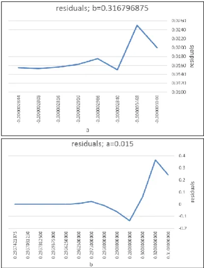
We find a and b by using the Runge-Kutta 4th code. As we see in Figure 1, (0,0) at the physical plane is transformed to (0,0) at the ζ plane. We use this node to find a and b. At first we assume that B (0.5,1) is transformed to b (1,0). A=(0.5,0) and F( ) d/dz then
2 2 2 2
( 1
/ a
) / (
)
d dz , therefore we need to find
the angle “a” to have F(ζ). As shown in Figure 2, we change assumed a, until the residual becomes constant. Residuals = abs[(assumed a-obtained a) / a].
Then, having the new a, we go to find b, and so on. Finally, a and b are obtained.
Figure 2. Convergence of calculation of a and b for α=1
4. CONVERGENCE
As mentioned before, to obtain one angle, another angle is guessed and by using the Runge-Kutta 4th code another angle is obtained. Then, the residual is calculated. After the first guessed angle is changed by adding slightly and again, second new angle is obtained.
As it can be observed from Figure 2, calculations continue until the residual reaches just around zero. In all graphs of the Figure 2, convergence is obvious.
5. RESULTS AND DISCUSSION
First, the code was written for a square cavity with the Reynolds number of 50. To compare our results, the FLUENT was used and the conformity was satisfactory. In the foregoing flow, the dimensionless velocity, u, plotted at the center line of the cavity and compared with the result of the FLUENT (Figure 3), which the agreement was perfect. The code was changed for the Reynolds number of 50000.
All of the parameters used in our code are listed in Table 1.
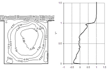
Formation of the primary eddy at the cavity center was observed (Figure 4). The primary eddy’s center was formed perfectly at the cavity’s center. In addition to formation of the two secondary eddies at the bottom of the cavity, there was another small eddy at the top left.
Figure 3. Average u velocity at centerline of cavity, (*) FLUENT, (-) code, at (Re=50 & α=1)
Figure 4. (Left): Stream lines of code, at Re= 50000 & α=1; (Right): average u velocity at centerline of cavity, (o) FLUENT, (-) code, at Re=50000
TABLE 1. Numerical parameters used in code
Reynolds number 50 50000
Δt (k) 0.05 0.05
h 0.2 0.05
Δx=Δy 0.02 0.02
Ys 1.4σ 2σ
Iterations 70 500 It.s for average vel. 20 300 Total iterations 90 800
Also, at this Reynolds number, the average velocity, u, was plotted at the center line of the cavity and compared with the FLUENT (Figure 4-right). In this condition, the coincidence was very good. The Κ-ω method was used for the turbulent flow and the convergence of the FLUENT results reached after 8000 iteration with residuals of k=0.5 ×10⁻⁴, ω=1 ×10⁻⁴, continuity=0.5 ×10⁻⁵ and xvel. & yvel. = 1 ×10⁻⁶.
In this figure, the instantaneous streamlines contours are shown as well. As noted, the contours do not have any regular shape which is another specification of turbulent flows. Incidentally, all primary and three secondary eddies are formed at the moment but have an irregular shape. As we know, having velocity fluctuations, Reynolds stresses can be obtained.
Also, for the cavity aspect ratio (α) equal 2, the same calculation was done for Re=50 and 50000. Figures 6 and 7 demonstrateboth the streamlines and comparison of the velocities center line obtained by the model and by the FLUENT. An acceptable agreement is observed.
Figure 5. (Left): Instantaneous stream lines of code; (Right): instantaneous u velocity of code at center line of cavity (Re= 50000 & α=1)
Figure 6. (Left): Stream lines of code, at Re= 50 & α=2; (Right): average u velocity at centerline of cavity, (o) FLUENT, (-) code, at Re=50000
Figure 7. (Left): Stream lines of code, at Re= 50000 & α=2; (Right): average u velocity at centerline of cavity, (o) FLUENT, (-) code, at Re=50000
6. CONCLUSION
A method to determine angles of the Schwarz-Christoffel mapping formula which is used in the Random Vortex Method is studied. Then, a code is written by RVM for an open square cavity and formation eddies is investigated in laminar and turbulent flows. Furthermore, dimensionless velocity at centerline of cavity is compared by FLUENT results. By using appropriate parameters, RVM is a very successful method in studying two-dimensional, viscous, incompressible and time dependent flows. Having instantaneous velocities, velocity fluctuations are achievable; consequently, Reynolds stresses can be calculated. Flow field -obtained by the Random Vortex Method- can be utilized in studying heat transfer and many other applications.
7. REFERENCES
1. Wolfshtein, M., "Some comments on turbulence modelling",
International Journal of Heat and Mass Transfer, Vol. 52, No. 17, (2009), 4103-4107.
2. Chorin, A.J., "Numerical study of slightly viscous flow",
Journal of Fluid Mechanics, Vol. 57, No. 4, (1973), 785-796. 3. Chorin, A.J., "Vortex sheet approximation of boundary layers",
Journal of Computational Physics, Vol. 27, No. 3, (1978), 428-442.
4. Chorin, A.J., "Vortex models and boundary layer instability",
SIAM Journal on Scientific and Statistical Computing, Vol. 1, No. 1, (1980), 1-21.
5. Sethian, J.A. and Ghoniem, A.F., "Validation study of vortex methods", Journal of Computational Physics, Vol. 74, No. 2, (1988), 283-317.
6. Beale, J.T., "A convergent 3-d vortex method with grid-free stretching", Mathematics of Computation, Vol. 46, No. 174, (1986), 401-424, S415.
7. Cottet, G.-H., "A new approach for the analysis of vortex methods in two and three dimensions", in Annales de l'Institut Henri Poincare (C) Non Linear Analysis, Elsevier. Vol. 5, (1988), 227-285.
8. Gharakhani, A. and Ghoniem, A.F., "Three-dimensional vortex simulation of time dependent incompressible internal viscous flows", Journal of Computational Physics, Vol. 134, No. 1, (1997), 75-95.
9. Ghoniem, A.F. and Cagnon, Y., "Vortex simulation of laminar recirculating flow", Journal of Computational Physics, Vol. 68, No. 2, (1987), 346-377.
10. Knio, O.M. and Ghoniem, A.F., "Three-dimensional vortex simulation of rollup and entrainment in a shear layer", Journal of Computational Physics, Vol. 97, No. 1, (1991), 172-223. 11. McCracken, M. and Peskin, C., "A vortex method for blood flow
through heart valves", Journal of Computational Physics, Vol. 35, No. 2, (1980), 183-205.
12. Summers, D., Hanson, T. and Wilson, C., "A random vortex simulation of wind‐flow over a building", International Journal for Numerical Methods in Fluids, Vol. 5, No. 10, (1985), 849-871.
approach", in 7th Symposium on Turbulent Shear Flows, Volume 1. Vol. 1, (1989), 10.13. 11-10.13. 15.
14. Ghoniem, A., Chorin, A. and Oppenheim, A., Numerical
modeling of turbulent flow in a combustion tunnel. 1980, Ernest
Orlando Lawrence Berkeley National Laboratory, Berkeley, CA (US).
15. Giovannini, A., Mortazavi, I. and Tinel, Y., "Numerical flow visualization in high reynolds numbers using vortex method computational results", ASME-PUBLICATIONS-FED, Vol. 218, No., (1995), 37-44.
16. Gagnon, Y., Giovannini, A. and Hébrard, P., "Numerical simulation and physical analysis of high reynolds number recirculating flows behind sudden expansions", Physics of Fluids A: Fluid Dynamics, Vol. 5, No. 10, (1993), 2377-2389. 17. Martins, L.-F. and Ghoniem, A.F., "Simulation of the
nonreacting flow in a bluff-body burner; effect of the diameter ratio", Journal of Fluids Engineering, Vol. 115, No. 3, (1993), 474-484.
18. Shokouhmand, H. and Sayehvand, H., "Numerical study of flow and heat transfer in a square driven cavity", International Journal of Engineering Transactions A: Basics, Vol. 17, No. 3, (2004), 301-317.
19. Taghilou, M. and Rahimian, M., "Simulation of lid driven cavity flow at different aspect ratios using single relaxation time lattice boltzmann method", (2013).
20. Zafarmand, B., Souhar, M. and Nezhad, A.H., "Analysis of the characteristics, physical concepts and entropy generation in a turbulent channel flow using vortex blob method", International Journal of Engineering, TRANSACTIONSA: Basics Vol. 29, No. 7, (2016), 985-994.
21. De, S. and Bathe, K.-J., "Towards an efficient meshless computational technique: The method of finite spheres",
Engineering Computations, Vol. 18, No. 1/2, (2001), 170-192. 22. Oppenheim, A.K., "Dynamics of combustion systems, Springer,
(2008).
Random Vortex Method for Geometries with Unsolvable
Schwarz-Christoffel
Formula
I. Tadayoni Navaeia, B. Zafarmandb
a Department of Mechanical Engineering, Mashhad Branch, Islamic Azad University, Mashhad, Iran bDepartment of Mechanical Engineering, Institute of Energy & Hydro Technology (IEHT), Mashhad, Iran
P A P E R I N F O
Paper history: Received 21 January 2017
Received in revised form 18 September 2017 Accepted 30 November 2017
Keywords: Flow Field
Numerical Simulation Open Cavity
Random Vortex Method Turbulent ديكچ ه ا رد نی قحت قی هبادرگ شور زا اه ی فداصت ی ارب ی م هبساحم نادی رج تعرس نای هرفح لخاد رد اه ی زاب ارب ی رج نای و مارآ
هبادرگ شور .تسا هدش هدافتسا مهرد اه ی فداصت ی کی تابساحم شور ی
م ود ره رد( تسا نادی
تهج هک )مهرد و مارآ
ن هب هسدنه لاقتنا می اب هحفص ،ییلا تشاگن زا Schwarz-Christoffel م هدافتسا ی خرب رد .دنک ی هسدنه زا اه ی پ هدیچی رج دننام نای تشاگن ،هرفح لخاد ی
ن هب ار هسدنه هک می لااب هحفص یی م لقتنم ی هب دنک ناسآ ی ب ه من تسد ی آ دی ا رد . نی هلاقم
ارب روکذم لاقتنا عبات ی
عبرم هرفح ی ضرع هب لوط تبسن اب( یلیطتسم و 2 ) ب ه ددع تروص ی ب ه م تسد ی آ دی سپس . ، م نادی اه ی هظحل تعرس ا ی هبادرگ شور طسوت هرفح لخاد طسوتم و اه ی فداصت ی م هبساحم ی وش ن ر دادعا .د زدلونی ارب ی رج نای اه ی ب مهرد و مارآ ه ترت بی 50 و 50000 دروم ود ره رد .تسا ،
زوت عی اتن اب لدم تعرس جی اقم تنئولف هسی م ی دوش هک سب رای اضر تی زم .دنتسه شخب تی
ا نی زاس لدم شور ی
ا تسنی ارب هک ی ،هسدنه زا هطقن ره رد تعرس هبساحم
تحا یجای دنب شم هب ی لک رد نایرج نادیم رد تعرس و هدوبن
کی م صاخ هطقن ی
قتسم دناوت می گتسباو نودب و ی طاقن هب د رگی ب ه آ تسد دی .