Proposed Procedure for Estimating the Coefficient of Three-factor Interaction for 2^p 3^m 4^q Factorial Experiments (TECHNICAL NOTE)

Please cite this article as: W. A. A. Alqraghuli, A. F. M. Alkarkhi, Y. Yusup, Proposed Procedure for Estimating the Coefficient of Three-factor Interaction for 2𝑝₃𝑚₄𝑞 _{Factorial Experiments, International Journal of Engineering (IJE), IJE TRANSACTIONS A: Basics Vol. 31, No. 1,} (January 2018) 12-18

International Journal of Engineering

J o u r n a l H o m e p a g e : w w w . i j e . i r

Proposed Procedure for Estimating the Coefficient of Three-factor Interaction for

2

3

4

Factorial Experiments

W. A. A. Alqraghulia_{, A. F. M. Alkarkhi}*b_{, Y. Yusup}c

a _{School of Mathematical Sciences, Universiti Sains Malaysia, Pulau Pinang, Malaysia}

b _{Malaysian Institute of Chemical & Bioengineering Technology Universiti Kuala Lumpur, (UniKL, MICET), Melaka, Malaysia} c _{School of Industrial Technology, Universiti Sains Malaysia, Pulau Pinang, Malaysia}

P A P E R I N F O

Paper history: Received 24 October 2017

Received in revised form 25 November 2017 Accepted 30 November 2017

Keywords:

Two-level Factorial Design Three-level Factorial Design Four-level Factorial Design Response Surface Models

A B S T R A C T

Three-factor interaction for the two-level, three-level, and four-level factorial designs was studied. A new technique and formula based on the coefficients of orthogonal polynomial contrast were proposed to calculate the effect of the three-factor interaction The results show that the proposed technique was in agreement with the least squares method. The advantages of the new technique are 1) it is fixed, 2) it is simple and 3) it is easy to apply without the complicated matrix formula of the least squares method. This new technique will also enhance the use of the coefficients of orthogonal contrast when analyzing other experimental designs.

doi: 10.5829/ije.2018.31.01a.02

1. INTRODUCTION1

Factorial design is widely applied in many fields because it is economical and efficient. It allows researchers to investigate the effects of several factors simultaneously. Moreover, the joint effects of factors on selected responses can be determined. Researchers in engineering and science fields have performed various experiments using this method, e.g., ferulic acid production by co-culture by Kamaliah & Norazwina [1] and response surface methodology for optimization experiments by Singh et al. [2], Kavardi et al. [3], Yahyaei et al. [4], Moradi et al. [5] and Maluta et al. [6].

The factorial design was proposed in the 1920s by Fisher [7] and became popular among researchers. In 1937, Yates suggested a method for analyzing two-level factorial designs [8], while Davies developed a procedure to fit a second-order response model to three-level factorial designs [9]. Some researchers suggested new methods to analyze different experiments while some researchers fitted response surface models to

*Corresponding Author’s Email: [email protected] (A. F. M. Alkarkhi)

various experiments. For instance, Margolin [10] developed a procedure to analyze and fit a response surface model to mixed-factorial designs for the two-level and three-two-level designs. Alkarkhi & Low [11] presented a procedure to analyze mixed experiments comprising of the two-level and three-level factorial designs by using the coefficients of the orthogonal polynomial contrast. Alqraghuli et al. [12] suggested a new method for analyzing four-level factorial designs and continued to introduce a new procedure to analyze mixed two-level and four-level factorial designs [13]. Later, Alqraghuli et al. [14] proposed a new procedure to analyze experiments of three-level and four-level designs.

The polynomial model is typically used to summarize the results gathered from experiments on mathematical models. It can similarly be used to understand the process behaviors of these models and the effects of various factors on them. Researchers applied the least squares method and matrix techniques to utilize polynomial models in factorial designs [15]. Subsequently, researchers developed a simpler but

accurate method by using the coefficients of the orthogonal polynomial.

The new procedures presented suggest an easy and simple method to avoid the difficulties and complication of using the least squares method, especially if more than two factors are involved, which would require the use of statistical software to fit the response surface model. The coefficients of orthogonal contrasts, to date, have never been used for analyzing mixed experiments of type two-level, three-level, and four-level experiments. Therefore, the objective of this work is to propose a new procedure for analyzing and fitting response surface models to mixed experiments of two-level, three-level and four-level factorial experiments and estimating the coefficient of the three-factor interaction.

2. 𝟐𝒑_𝟑𝒎_𝟒𝒒 _{FACTORIAL DESIGN}

The mixed experiment of type two-level, three-level and four-level are denoted by 2𝑝₃𝑚₄𝑞_{, 𝑝 factors each at two} levels 𝑋1, … , 𝑋𝑝, 𝑚 factors each at three levels 𝑍1,… 𝑍𝑚 and 𝑞 factors each at four levels 𝑅1, … , 𝑅𝑠. The simplest design for two-level, three-level and four-level, factorial design has three factors, one at two levels one at three levels and one at four levels 21₃1₄1_{. The total number} of runs required for 21₃1₄1 _{is 24 runs for one replicate} [16].

3. PROPOSED PROCEDURE

Many researchers have studied different factorial designs to develop formulas or by offering new techniques. Experiments of type 2𝑝₃𝑚₄𝑞_{have not been} considered using the coefficients of orthogonal polynomial contrasts. Thus, this work will propose a new procedure for analyzing and fitting response surface models to this type of experiments and introduce a new formula for estimating the coefficient of the three-factor interaction.

Consider three types of factors, the first type is of two-level (𝑋1, … , 𝑋𝑝), the second type is of three-level (𝑍1,… 𝑍𝑚) and the last type is of four-level (𝑅1… , 𝑅𝑞). Thus, the design that considers all three types of factors is called experiment of type 2𝑝₃𝑚₄𝑞_{. The proposed} procedure splits the experiment into three experiments, one of type 2𝑝, the second is of type 3𝑚 and the third is of type 4𝑞_{, then analyzing each experiment separately.} The coefficients of the linear effect and two-factor interaction in the response surface models are estimated using the formulas for analyzing experiments of type 2𝑝_{, experiment of type 3}𝑚_{, experiment of type 4}𝑞 _[14], experiments of type 2𝑝₃𝑚 _{[13], experiments of type}

2𝑝₄𝑞 _{[10], and experiment of type 3}𝑚₄𝑞 _{[13], which are}

based on the coefficients of orthogonal polynomial contrast. We need to propose a formula for estimating the coefficient of the three-factor interaction to cover all coefficients in the model. The recommended procedure for calculating the coefficients of the three-factor interaction depends on the coefficients of orthogonal polynomial contrasts for twolevel 1, 1, for threelevel -1, 0, -1, and for four-level -3, --1, -1, 3.

The formulas for fitting two-level factorial designs to the response surface model are given in Equations (1) and (2) for estimating the coefficients of the linear effect and two-factor interaction respectively as:

𝑏𝑙=

𝑐𝑜𝑛𝑡𝑟𝑎𝑠𝑡 𝑓𝑜𝑟𝐴𝑙

4𝑛 𝑙 = 1, 2, … , 𝑝 (1)

𝑏𝑙𝑞=

𝐶𝑜𝑛𝑡𝑟𝑎𝑠𝑡 𝑓𝑜𝑟 𝐴𝑙𝐴𝑞

4𝑛 𝑙 ≠ 𝑞 (2)

where 𝑛 represents the number of replicates at each level or the number of replicates at the joint levels in case of interaction between different factors.

The formulas for fitting three-level factorial designs to the response surface model are given in Equations (3)-(5) for estimating the coefficients of the linear effect, two-factor interaction and the quadratic coefficients respectively as defined:

𝛾𝑟=

𝑙𝑖𝑛𝑒𝑎𝑟 𝑐𝑜𝑛𝑡𝑟𝑎𝑠𝑡 𝑓𝑜𝑟 𝐴𝑟

2𝑛 𝑟 = 1, 2, … , 𝑚 (3)

𝛾𝑟𝑟=𝑄𝑢𝑎𝑑𝑟𝑎𝑡𝑖𝑐 𝑐𝑜𝑛𝑡𝑟𝑎𝑠𝑡 𝑓𝑜𝑟 𝐴_2𝑛 𝑟𝑟 (4)

𝛾𝑟𝐿=

𝑙𝑖𝑛𝑒𝑎𝑟 𝑐𝑜𝑛𝑡𝑟𝑎𝑠𝑡 𝑓𝑜𝑟 𝐴𝑟𝐴𝐿

4𝑛 𝑟 ≠ 𝐿 (5)

The formulas for fitting four-level factorial designs to the response surface model are given in Equations (6)-(8) for estimating the coefficients of the main effect, two-factor interaction and the quadratic coefficients, respectively, as defined by Alqraghuli et al. [14].

𝛽𝑠=𝐿𝑖𝑛𝑒𝑎𝑟 𝑐𝑜𝑛𝑡𝑟𝑎𝑠𝑡 𝑓𝑜𝑟𝐴_20×𝑛 𝑠 𝑠 = 1, 2, … , 𝑞 (6)

𝛽𝑠𝑠=𝑄𝑢𝑎𝑑𝑟𝑎𝑡𝑖𝑐 𝑐𝑜𝑛𝑡𝑟𝑎𝑠𝑡 𝑓𝑜𝑟 𝐴_16×𝑛 𝑠𝑠 (7)

𝛽𝑠𝑡=𝐿𝑖𝑛𝑒𝑎𝑟 𝑐𝑜𝑛𝑡𝑟𝑎𝑠𝑡 𝑓𝑜𝑟 𝐴_400𝑛 𝑠𝐴𝑡 𝑠 ≠ 𝑡 (8)

The formula for estimating the linear coefficient of the two-factor interaction for the mixed experiment of type two-level and three-level factorial designs is given in Equation (9) as defined by Alkarkhi & Low [11].

𝛼𝑙𝑟=𝐿𝑖𝑛𝑒𝑎𝑟 𝑐𝑜𝑛𝑡𝑟𝑎𝑠𝑡 𝑓𝑜𝑟𝐴_4𝑛 𝑙𝐴𝑟 𝑙 = 1, 2, … , 𝑝 𝑟 =

1, 2, … , 𝑚 (9)

𝜃𝑙𝑠=

𝐿𝑖𝑛𝑒𝑎𝑟 𝑐𝑜𝑛𝑡𝑟𝑎𝑠𝑡 𝑓𝑜𝑟 𝐴𝑙𝐴𝑠

40×𝑛 𝑙 = 1, 2, … , 𝑝 𝑠 =

1, 2, … , 𝑞 (10)

The formula for estimating the linear coefficient of the two-factor interaction for the mixed experiment of type three-level and four-level factorial designs is given in Equation (11) as defined by Alqraghuli et al. [12].

𝛿

=

𝐿𝑖𝑛𝑒𝑎𝑟 𝑐𝑜𝑛𝑡𝑟𝑎𝑠𝑡 𝑓𝑜𝑟 𝐴_𝑟𝐴_𝑠

40𝑛

𝑟 = 1, 2, … , 𝑚 𝑠 = 1, 2, … , 𝑞

(11)

The next step is to derive a formula for calculating the linear coefficient of three-factor interaction between factor at two-level, factor at three-level and factor at four-level.

3. 1. Derive The Proposed Formula Suppose there are 𝑝 factors each at two levels 𝑋1, 𝑋2, … , 𝑋𝑝,𝑚 factors each at three levels 𝑍1, 𝑍2, … , 𝑍𝑚 and 𝑞 factors each at four levels 𝑅1,𝑅2,… , 𝑅𝑞, consider a response surface model in Equation (12).

𝑌𝑖 =

𝑏0∑𝑝𝑙=1𝑏𝑖𝑋𝑙𝑖+

∑ ∑𝑙<𝑗𝑏𝑙𝑗𝑋𝑙𝑖𝑋𝑗𝑖+∑𝑚𝑟=1𝛾𝑟𝑍𝑟𝑖+∑𝑚𝑟=1𝛾𝑟𝑟𝑍𝑟𝑖2 +

∑ ∑𝑟<𝐿𝛾𝑟𝐿𝑍𝑟𝑖𝑍𝐿𝑖+ ∑𝑠=1𝑞 𝛽𝑠𝑅𝑠𝑖+ ∑𝑞𝑠=1𝛽𝑠𝑠𝑅𝑠𝑖2 +

∑ ∑𝑠<𝑡𝛽𝑠𝑡𝑅𝑠𝑖𝑅𝑡𝑖+

∑𝑙=1𝑝 ∑𝑟=1𝑚 𝛼𝑙𝑟𝑋𝑙𝑖𝑍𝑟𝑖+∑ ∑𝑞𝑠=1𝜃𝑙𝑠𝑋𝑙𝑖𝑅𝑠𝑖

𝑝

𝑙=1 +

∑𝑟=1𝑚 ∑𝑠=1𝑞 𝛿𝑟𝑠𝑍𝑟𝑖𝑅𝑠𝑖+ ∑𝑙=1𝑝 ∑𝑟=1𝑚 ∑𝑞𝑠=1𝜏𝑙𝑟𝑠𝑋𝑙𝑖𝑍𝑟𝑖𝑅𝑠𝑖

𝑖 = 1, … , 𝑘

(12)

The model in Equation (12) should satisfy some constraints regarding each type of the selected factors. The constraints are based on the coefficients of orthogonal polynomial contrast.

1. The constraints for the factors at two levels are: 1. ∑𝑘𝑖=1𝑋𝑙𝑖 = 0 2. ∑𝑘𝑖=1𝑋𝑙𝑖𝑋𝑗𝑖= 0 3. ∑𝑘𝑖=1𝑋𝑙𝑖2𝑋𝑗𝑖= 0 4.∑𝑘𝑖=1𝑋𝑙𝑖𝑋𝑗𝑖2= 0 5. ∑𝑘𝑖=1𝑋𝑙𝑖𝑋𝑗𝑖𝑋ℎ𝑖= 0 6.∑ 𝑋𝑘𝑖 𝑖2= 𝑘 7. ∑𝑘𝑖=1(𝑋𝑙𝑖𝑋𝑗𝑖)2= 𝑘

2. The constraints for the factors at three levels are: 1.∑𝑘𝑖=1𝑍𝑖= 0 2. ∑𝑖=1𝑘 𝑍𝑟𝑖𝑍𝐿𝑖 = 0 3. ∑𝑘𝑖=1𝑍𝑟𝑖2𝑍𝐿𝑖 = 0 4. ∑𝑘𝑖=1𝑍𝑟𝑖𝑍𝐿𝑖2 = 0 5. ∑𝑘𝑖=1𝑍𝑟𝑖𝑍𝐿1𝑍ℎ𝑖 = 0

6. ∑𝑘𝑖=1𝑍𝑟𝑖2 = ∑𝑘𝑖=1𝑍𝑟𝑖4 = 2 × 3𝑚−1 7. ∑𝑘𝑖=1(𝑍𝑟𝑖𝑍𝐿𝑖)2= 4 × 3𝑚−2

3. The constraints for factors at four levels are: 1. ∑𝑘𝑖=1𝑅𝑠𝑖= 0 2. ∑𝑖=1𝑘 𝑅𝑠𝑖𝑅𝑡𝑖= 0 3. ∑𝑘𝑖=1𝑅𝑠𝑖𝑅𝑡𝑖2 = 0 4. ∑𝑘𝑖=1𝑅𝑠𝑖𝑅𝑡𝑖2 = 0 5. ∑𝑘𝑖=1𝑅𝑠𝑖2 = 20 × 4𝑞_1

6. ∑𝑘𝑖=1𝑅𝑠𝑖4 = 164 × 4𝑞_1 7. ∑𝑘𝑖=1𝑅𝑠𝑖2𝑅𝑡𝑖2 = 400 × 4𝑞_2 8. ∑𝑘𝑖=1𝑅𝑠𝑖𝑅𝑡𝑖𝑅ℎ𝑖 = 0 9. ∑𝑘𝑖=1(𝑅𝑠𝑖𝑅𝑡𝑖)2= 400 × 4𝑞−2

4. The constraints for the joint effects between factors at two levels and factors at four levels are:

1. ∑𝑘𝑖=1(𝑅𝑠𝑖𝑋𝑙𝑖)2= 40 × (4𝑞−1× 2𝑝−1) 2. ∑𝑘𝑖=1𝑋𝑙𝑖𝑅𝑠𝑖= ∑𝑘𝑖=1𝑋𝑙𝑖2𝑅𝑠𝑖= ∑𝑘𝑖=1𝑋𝑙𝑖𝑅𝑠𝑖2 = 0 3. ∑𝑘𝑖=1𝑋𝑙𝑖𝑋𝑗𝑖𝑅𝑠𝑖= ∑𝑘𝑖=1𝑅𝑠𝑖𝑅𝑡𝑖𝑋𝑙𝑖 = 0

5. The constraints for the joint effects between factors at three levels and factors at four levels are:

1. ∑𝑖=1𝑘 (𝑍𝑟𝑖𝑅𝑠𝑖)2=40× (4𝑞−1× 3𝑚−1)

2. ∑𝑘𝑖=1𝑍𝑟𝑖𝑅𝑠𝑖= ∑𝑖=1𝑘 𝑍𝑟𝑖2𝑅𝑠𝑖= ∑𝑘𝑖=1𝑍𝑟𝑖𝑅𝑠𝑖2 = 0 3. ∑𝑘𝑖=1𝑍𝑟𝑖𝑍𝑗𝑖𝑅𝑠𝑖= ∑𝑘𝑖=1𝑅𝑠𝑖𝑅𝑡𝑖𝑍𝑙𝑖 = 0

6. The constraints for the joint effects between factors at two levels, three levels and four levels are:

1. ∑𝑘𝑖=1𝑋𝑙𝑖𝑍𝑟𝑖𝑅𝑠𝑖= 0 2. ∑𝑘𝑖=1𝑋𝑙𝑖2𝑍𝑟𝑖𝑅𝑠𝑖= 0

3. ∑𝑘ℎ<𝑗<𝑙𝑋ℎ𝑖𝑍𝑗𝑖2𝑅𝑙𝑖 = 0 4. ∑𝑘𝑖=1𝑋𝑙𝑖𝑍𝑟𝑖𝑅𝑠𝑖2 = 0 5. ∑𝑘𝑖=1𝑋𝑙𝑖𝑍𝑟𝑖3𝑅𝑠𝑖= 0 6. ∑𝑘𝑖=1𝑋𝑙𝑖𝑍𝑟𝑖𝑅𝑠𝑖3 = 0

7. ∑𝑘𝑖=1𝑋𝑙𝑖2𝑍𝑟𝑖2𝑅𝑠𝑖= 0 8. ∑𝑘𝑖=1𝑋𝑙𝑖2𝑍𝑟𝑖𝑅𝑠𝑖2 9. ∑𝑘𝑖=1𝑋𝑙𝑖𝑍𝑟𝑖2𝑅𝑠𝑖2

10. ∑𝑘𝑖=1𝑋𝑙𝑖2𝑍𝑟𝑖2𝑅𝑠𝑖2 = 32 × 2𝑝× 3𝑚−1× 4𝑞−1 11. ∑(𝑋1𝑖𝑍1𝑖𝑅1𝑖)2= 80 × (2𝑝−13𝑚−14𝑞−1)

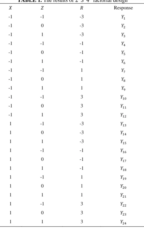
To illustrate the procedure, consider a 21₃1₄1 experiment without losing information for the general case. Suppose there are three factors, 𝑋1 at two levels,

𝑍1 at three levels and 𝑅1 at four levels. The response surface model that describes the relationship between the selected factors and the response is given in Equation (13).

𝑌𝑖= 𝑏0+ 𝑏1𝑋1𝑖+ 𝛾1𝑍1𝑖+ 𝛾11𝑍1𝑖2 +

𝛽1𝑅1𝑖+ 𝛽11𝑅1𝑖2 + 𝛼11𝑋1𝑖𝑍1𝑖+ 𝜃11𝑋1𝑖𝑅1𝑖+

𝛿11𝑍1𝑖𝑅1𝑖+ 𝜏111𝑋1𝑖𝑍1𝑖𝑅1𝑖 𝑖 = 1 ,2, … , 𝑘

(13)

The treatment combinations of this experiment are given in Table 1.The levels of the selected factors are represented by -1 and 1 for two-level factor, -1, 0, and 1 for three-level factor and -3, -1, 1, and 3 for four-level factor.

The proposed procedure depends on partitioning the experiment into three experiments according to the type of factors under study. Thus, two-level can be considered as 21_{factorial design, three-level can be} considered as 31 _{factorial design and four-level can be} considered as 41 _{factorial design. Then, analyze each} experiment separately to estimate the linear and quadratic coefficients while the coefficient of the two-factor interaction can be evaluated by studying the combination between any two types as presented earlier. Three-factor interaction between factors that have two levels, three levels and factors that have four levels can be studied by constructing 𝐶1

𝑝

𝐶1𝑚𝐶1 𝑞

experiments of the form 21₃1₄1

applying the constraints will result in 𝜏111 in Equation (14).

TABLE 1. The results of 21₃1₄1 _{factorial design}

𝑋 𝑍 𝑅 Response

-1 -1 -3 𝑌1

-1 0 -3 𝑌2

-1 1 -3 𝑌3

-1 -1 -1 𝑌4

-1 0 -1 𝑌5

-1 1 -1 𝑌6

-1 -1 1 𝑌7

-1 0 1 𝑌8

-1 1 1 𝑌9

-1 -1 3 𝑌10

-1 0 3 𝑌11

-1 1 3 𝑌12

1 -1 -3 𝑌13

1 0 -3 𝑌14

1 1 -3 𝑌15

1 -1 -1 𝑌16

1 0 -1 𝑌17

1 1 -1 𝑌18

1 -1 1 𝑌19

1 0 1 𝑌20

1 1 1 𝑌21

1 -1 3 𝑌22

1 0 3 𝑌23

1 1 3 𝑌24

∑ 𝑋1𝑖𝑍1𝑖𝑅1𝑖𝑌𝑖= 𝜏111∑(𝑋1𝑖𝑍1𝑖𝑅1𝑖)2

𝜏111=

∑ 𝑋1𝑖𝑍1𝑖𝑅1𝑖𝑌𝑖

∑(𝑋1𝑖𝑍1𝑖𝑅1𝑖)2 (14)

Equation (14) can be written in the form of the coefficients of orthogonal polynomial contrast. Let us start with the denominator of Equation (14). The denominator of Equation (14) is equal to:

∑(𝑋1𝑖𝑍1𝑖𝑅1𝑖)2= 80 × (2𝑝−13𝑚−14𝑞−1)

= 80 × (21−1₃1−1₄1−1_{) = 80 × 1}

where 1 represents the number of replicates. The numerator of Equation (14) is

∑24𝑖=1𝑋1𝑖𝑍1𝑖𝑅1𝑖𝑌𝑖=

(−1)(−1)(−3)𝑌1+ (−1)(0)(−3)𝑌2+

(−1)(1)(−3)𝑌3+ ⋯ + (1)(1)(3)𝑌24 = −3(𝑌1+ 𝑌12+

𝑌15+ 𝑌22) − 1(𝑌4+𝑌9+𝑌18+𝑌19) + 0(𝑌2+𝑌5+

𝑌8+𝑌11+ 𝑌14+ 𝑌17+𝑌20+𝑌23) + 1(𝑌6+ 𝑌7+ 𝑌16+

𝑌21) + 3(𝑌3+ 𝑌10+ 𝑌13+ 𝑌24)

The result of the numerator of Equation (14) is similar to the result of using the coefficients of linear contrasts

of selected factors (linear joint contrast for 𝑋1, 𝑍1 and

𝑅1). The formula for estimating the three-factor interaction regarding the coefficients of orthogonal polynomial contrast is given in Equation (15).

𝜏111=

∑ 𝑋1𝑖𝑍1𝑖𝑅1𝑖𝑌𝑖

∑(𝑋1𝑖𝑍1𝑖𝑅1𝑖)2=

𝐿𝑖𝑛𝑒𝑎𝑟 𝑐𝑜𝑛𝑡𝑟𝑎𝑠𝑡 𝑓𝑜𝑟 𝑋1𝑍1𝑅1

80×1 (15)

In general, let 𝑛 represents the number of replicates at the joint levels. Equation (15) becomes as below:

𝜏𝑙𝑟𝑠=

𝐿𝑖𝑛𝑒𝑎𝑟 𝑐𝑜𝑛𝑡𝑟𝑎𝑠𝑡 𝑓𝑜𝑟𝐴𝑙𝐴𝑟𝐴𝑠

80×𝑛 (16)

The formula for estimating the intercept (𝑏0) in response surface model is given in Equation (17) which can be derived by summing Equation (13) over 𝑖 and applying all the constraints presented earlier; the result will be the formula for 𝑏0 as given in Equation (17).

𝑏0= 𝑌̅ − 𝛾11𝑍̅1− 𝛽11𝑅̅1 (17)

In general, in case of 𝑚 three-level factors and 𝑞 four-level factor are included in the model, Equation (17) becomes:

𝑏0= 𝑌̅ − 𝛾11𝑍̅1− ⋯ − 𝛾𝑚𝑚𝑍̅𝑚− 𝛽11𝑅̅1− ⋯ − 𝛽𝑞𝑞𝑅̅𝑞

where 𝑍̅ =∑ 𝑍𝑖2

𝑘 , 𝑅̅ =

∑ 𝑅_𝑖2

𝑘 , and 𝑘 is the total number of observations.

4. APPLICATION

Arbitrary data was used to illustrate the new procedure for analyzing the mixed experiment of type two-level, three-level, and four-level factorial design and estimating the linear coefficient of three-factor interaction. The effect of three factors, operating time (𝑋1) at two levels (30 and 60 min), current applied (𝑍1) at three levels (0.3, 0.4, 50 A), and inter-electrode (𝑅1) at four levels (0.5, 1, 1.5, 2 cm) on wastewater treatment by using electro-coagulation on power consumption (𝑌) was studied. Two replicates were used to run the experiment. Thus, the total number is (21₃1₄1_{) × 2 = 48} runs. The levels of each factor in actual and coded form are given in Table 2.

Fitting a response surface model to this type of experiment requires applying the procedures presented earlier.

TABLE 2. The actual and coded form for the selected

variables

Inter-electrode 0.5 1 1.5 2

Coded -3 -1 1 3

Current applied 0.3 0.4 0.5

Coded -1 0 1

Coded -1 1

The response surface model that describes the relationship between power consumption (𝑌) and selected factors is given in Equation (18).

𝑌𝑖= 𝑏0+ 𝑏1𝑋1𝑖+ 𝛾1𝑍1𝑖+ 𝛽1𝑅1𝑖+ 𝛾11𝑍1𝑖2+

𝛽11𝑅1𝑖2 + 𝛼11𝑋1𝑖𝑍1𝑖+ 𝜃11𝑋1𝑖𝑅1𝑖+ 𝛿11𝑍1𝑖𝑅1𝑖+

𝜏111𝑋1𝑖𝑍1𝑖𝑅1𝑖

(18)

Let us analyze the two-level factorial design first. The linear coefficient 𝑏1 is:

𝑏1=

𝐿𝑖𝑛𝑒𝑎𝑟 𝑐𝑜𝑛𝑡𝑟𝑎𝑠𝑡 𝑓𝑜𝑟 𝑋1

2×𝑛 =

35.3

2×24= 0.74 where the linear contrast (L) for 𝑋1 is

𝐿𝑋1= (−1)(1809) + (1)(1844.3) = 35.3 and 𝑛 = 24 represents the number of observations at each level of the two-level factorial design.

𝛾1=

𝐿𝑖𝑛𝑒𝑎𝑟 𝑐𝑜𝑛𝑡𝑟𝑎𝑠𝑡 𝑓𝑜𝑟 𝑍1

2𝑛 =

47.5

2×16= 1.484 where 𝐿𝑍1= (−1)(1188.6) + (0)(1228.6) +

(1)(1236.1) = 47.5. 𝛾11=

𝑄𝑢𝑎𝑑𝑟𝑎𝑡𝑖𝑐 𝑐𝑜𝑛𝑡𝑟𝑎𝑠𝑡 𝑓𝑜𝑟 𝑍1

2𝑛 =

−32.5

2×16= −1.016 where 𝑄𝑍1= (1)(1188.6) − (2)(1228.6) +

(1)1236.1 = −32.5.

and 𝑛 = 16 represents the number of observations at each level of the three-level factorial design.

The third experiment is of type four-level factorial design. The linear (L) and quadratic contrast (Q) are: 𝛽1=

𝐿𝑖𝑛𝑒𝑎𝑟 𝑐𝑜𝑛𝑡𝑟𝑎𝑠𝑡 𝑓𝑜𝑟 𝑅1

20×𝑛 =

480.9

20×12= 2.004

where L𝑅1=− 3(729.5) + −(1064.9) + (921.2) +

3(937.7) = 480.9 𝛽11=

𝑄𝑢𝑎𝑑𝑟𝑎𝑡𝑖𝑐 𝑐𝑜𝑛𝑡𝑟𝑎𝑠𝑡 𝑓𝑜𝑟 𝑅1

16×𝑛 =

−318.9

16×12= −1.66

where 𝑄𝑅1= (1)(729.5) + (−1)(1064.9) +

(−1)(921.2) + (1)(937.7) = −318.9

and 𝑛 = 12 represents the number of observations at each level of the four-level factorial design.

Next step is to analyze combined experiment to calculate the coefficient of two-factor interaction. The first two-factor interaction is between 𝑋1 and 𝑍.

The coefficient of two-factor interaction between 𝑋1 and

𝑍1 is:

𝛼11=

𝐿𝑖𝑛𝑒𝑎𝑟 𝑐𝑜𝑛𝑡𝑟𝑎𝑠𝑡 𝑓𝑜𝑟 𝑋₁𝑍₁

4𝑛 =

−141.3

4×8 = −4.416 where 𝐿𝑋₁𝑍₁= (−1)(−1)(567.9) + (1)(−1)(620.7) +

⋯ + (1)(573.8) = −141.3

and 𝑛 = 8 represents the number of observations at each joint level of the mixed two-level and three-level factorial design.

The two-factor interaction between 𝑋1 and 𝑅1 is:

𝜃11=

𝐿𝑖𝑛𝑒𝑎𝑟 𝑐𝑜𝑛𝑡𝑟𝑎𝑠𝑡 𝑓𝑜𝑟 𝑋1𝑅1

40𝑛 =

−45.1

40×6 = −0.188 where

L𝑋1𝑅1= (−1)(−3)(343.5) + (−1)(−1)(555.7) +

⋯ + (1)(1)(481.1) = −45.1

and 𝑛 = 6, represents the number of observations at each joint level of the two-level and four-level factorial design.

The coefficient of two-factor interaction between three-level and four-level factors 𝑍1𝑅1 is given below:

𝛿11=

𝐿𝑖𝑛𝑒𝑎𝑟 𝑐𝑜𝑛𝑡𝑟𝑎𝑠𝑡 𝑓𝑜𝑟 𝑍1𝑅1

40𝑛 =

−519.9

40×4 = −3.249 = where 𝐿𝑍1𝑅1=(−1)(−3)(190.7)+⋯+(1)(3)(259.5)=−519.9

The coefficient of the three-factor interaction between 𝑋1 𝑍1 𝑎𝑛𝑑 𝑅1 is calculated as defined in Equation (16).

L𝑋1𝑍1𝑅1= (−1)(−1)(−3)(87.1) + ⋯ +

((1)(1)(3)(111) = −4.3 𝜏111=

𝐿𝑖𝑛𝑒𝑎𝑟 𝑐𝑜𝑛𝑡𝑟𝑎𝑠𝑡 𝑓𝑜𝑟 𝑋1𝑍1𝑅1

80𝑛 =

−4.3

80×2= −0.027 The last coefficient of Equation (18) is the intercept 𝑏0 which is calculated as defined in Equation (17):

𝑌̅ =∑ 𝑌

𝑛 = 76.1104 𝑍̅ = ∑ 𝑍_𝑖2

𝑘 = 0.667

𝑅̅ =∑ 𝑅𝑖2

𝑘 = 5

𝑏0=𝑌̅ − 𝛾11𝑍̅1− 𝑎11𝑅̅1

𝑏0= 76.1104 − (−1.016)(0.667) − (−1.66)(5) =

85.0915

The fitted response surface model that describes the relationship between the power consumption and time and current applied in Equation (18) is given below: 𝑌 = 85.12 + 0.74𝑋1+ 1.484𝑍1+ 2.004𝑅1−1.016𝑍12−

1.66𝑅12− 4.416𝑋1𝑍1− 0.188𝑋1𝑅1−3.249𝑍1𝑅1−

0.027𝑋1𝑍1𝑅1

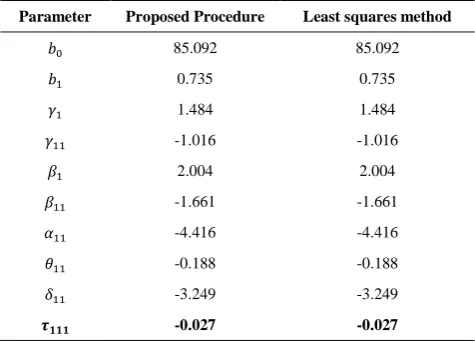
The experiment was also analyzed using the least squares method [18, 19]. The results of using the least squares were in agreement with the proposed procedure for three-factor interaction (𝜏111) as presented in Table 3.

5. CONCLUSION

Based on the results, it can be said that the coefficients of orthogonal polynomial contrast can be used for fitting response surface models without the complication of using the least squares method.

TABLE 3. The coefficients of the model calculated by the

least squares and proposed methods

Parameter Proposed Procedure Least squares method

𝑏0 85.092 85.092

𝑏1 0.735 0.735

𝛾1 1.484 1.484

𝛾11 -1.016 -1.016

𝛽1 2.004 2.004

𝛽11 -1.661 -1.661

𝛼11 -4.416 -4.416

𝜃11 -0.188 -0.188

𝛿11 -3.249 -3.249

Furthermore, this result will enhance the use of coefficients of orthogonal polynomial contrast in analyzing different experimental designs and provide simple and easy formulas removing the dependence on statistical software.

6. REFERENCES

1. Samad, K.A. and Zainol, N., "The use of factorial design for ferulic acid production by co-culture", Industrial Crops and Products, Vol. 95, (2017), 202-206.

2. Singh, R., Rizvi, S. and Tewari, S., "Effect of friction stir welding on the tensile properties of aa6063 under different conditions", International Journal of Engineering-Transactions A: Basics, Vol. 30, No. 4, (2017), 597-603.

3. Kavardi, S.S., Alemzadeh, I. and Kazemi, A., "Optimization of lipase immobilization", International Journal of Engineering, Transactions A: Basics, Vol. 25, No. 1, (2012), 1-9.

4. Yahyaei, M., Bashiri, M. and Garmeyi, Y., "Multi-criteria logistic hub location by network segmentation under criteria weights uncertainty", International Journal of Engineering, Vol. 27, No. 8, (2014), 1205-1214.

5. Moradi, M., Zinatizadeh, A.A. and Zinadini, S., "Influence of operating variables on performance of nanofiltration membrane for dye removal from synthetic wastewater using response surface methodology", International Journal Engineering. Transactions C: Aspects, Vol. 29, No. 12 (2016), 1650-1658.

6. Maluta, F., Eaglesham, A., Jones, D., Komrakova, A. and Kresta, S.M., "A novel factorial design search to determine realizable constant sets for a multi-mechanism model of mixing sensitive precipitation", Computers & Chemical Engineering, Vol. 106, (2017), 322-338.

7. Addelman, S., "Recent developments in the design of factorial experiments", Journal of the American Statistical Association, Vol. 67, No. 337, (1972), 103-111.

8. Yates, F., "The design and analysis of factorial experiments, Imperial Bureau of Soil Science, (1978).

9. Davies, O.L., "The design and analysis of industrial experiments", The Design and Analysis of Industrial Experiments., (1954), 234-251..

10. Margolin, B.H., "Systematic methods for analyzing 2 n 3 m factorial experiments with applications", Technometrics, Vol. 9, No. 2, (1967), 245-259.

11. Alkarkhi, A.F. and Low, H., "A proposed technique for analyzing experiments of type", Modern Applied Science, Vol. 3, No. 1, (2008), 95-102.

12. Alqaraghuli, W.A., Alkarkhi, A.F. and Low, H., "A new procedure for fitting second-order model to four-level factorial designs", World Applied Sciences Journal, Vol. 22, No. 8, (2013), 1116-1128.

13. Alqraghuli, W.A.A., Alkarkhi, A.F.M. and Low, H.C., "Fitting second-order models to mixed two-level and four-level factorial designs: Is there an easier procedure?", International Journal of Engineering,Transsactions B: Application, Vol. 28, No. 11, (2015), 1644-1650.

14. Alqraghuli, W.A.A., Alkarkhi, A.F.M. and Low, H.C., "Fitting second-order model to mixed three-level and four-level factorial designs using the coefficient of polynomial contrast", World Applied Sciences Journal, Vol. 33, No. 9, (2015), 1450-1456. 15. Draper, N.R. and Stoneman, D.M., "Response surface designs

for factors at two and three levels and at two and four levels",

Technometrics, Vol. 10, No. 1, (1968), 177-192.

Proposed Procedure for Estimating the Coefficient of Three-factor

Interaction for

2

3

4

Factorial Experiments

TECHNICAL NOTE

W. A. A. Alqraghulia_{, A. F. M. Alkarkhi}b_{, Y. Yusup}c

a _{School of Mathematical Sciences, Universiti Sains Malaysia, Pulau Pinang, Malaysia}

b _{Malaysian Institute of Chemical & Bioengineering Technology Universiti Kuala Lumpur, (UniKL, MICET), Melaka, Malaysia} c _{School of Industrial Technology, Universiti Sains Malaysia, Pulau Pinang, Malaysia}

P A P E R I N F O

Paper history: Received 24 October 2017

Received in revised form 25 November 2017 Accepted 30 November 2017

Keywords:

Two-level Factorial Design Three-level Factorial Design Four-level Factorial Design Response Surface Models

ديكچ ه

.تفرگ رارق هعلاطم دروم حطس راهچ و حطس هس ،حطس ود لیروتکاف یاه حرط یارب لماع هس لماعت لومرف و شور کی

یم ناشن جیاتن .تسا هدش داهنشیپ لماع هس لباقتم رثا هبساحم یارب دماعتم یا هلمجدنچ تسارتنک بیارض رب ینتبم دیدج

هک دهد :زا دنترابع دیدج شور یایازم .دراد تقباطم عبرم نیرتکچوک شور اب یداهنشیپ شور 1

،تسا هدش تیبثت نآ )

2 و تسا هداس ) 3

،نینچمه.تسا ناسآ عبرم نیرتکچوک شور هدیچیپ سیرتام لومرف نودب نآ زا هدافتسا ) شور نیا

حرط ریاس لیلحت ماگنه ار لداعتم تسارتنک بیارض زا هدافتسا دیدج .دهد یم شیازفا یبرجت یاه