Analysis of Building Electric Energy Consumption Data Using an Improved Cooling Degree Day Method

Analysis of Building Electric Energy Consumption Data Using an

Improved Cooling Degree Day Method

Krese, G. – Prek, M. – Butala, V.

Gorazd Krese – Matjaž Prek* _{– Vincenc Butala}

University of Ljubljana, Faculty of Mechanical Engineering, Slovenia

In cases where a quick insight into the operation of an HVAC system is more important than accuracy, cooling degree days can be used for monitoring electric energy consumption dependent on meteorological conditions. Cooling degree days are calculated from differences between outdoor temperatures above the base temperature and the base temperature itself, therefore containing both climate and building information. The difficulties in applying this method are the determination of base temperature and choosing a procedure for calculating degree days, which vary depending on the resolution of the weather data used. In addition, the cooling degree method has a major flaw, i.e. it considers only a linear dependence between cooling energy consumption and sensible cooling load, thereby ignoring latent loads, which become more significant at higher outdoor temperatures.

In this article an analysis of real electric energy consumption data using the cooling degree method and an improved method derived from it that includes latent loads, as well as a comparison between them, are shown. Both methods are applied several times to metered data, each time with a different combination of a method for determining base temperature and a degree day calculation technique.

Keywords: building electric energy consumption, cooling degree day, base temperature, latent load, wet-bulb temperature

0 INTRODUCTION

One of the targets of the European Union (EU) growth strategy Europe 2020 is to reduce greenhouse gas (GHG) emissions by at least 20% compared to 1990 levels, increase the share of renewable energy sources in final energy consumption to 20% and to reduce the primary energy use by 20% with projected levels by 2020 (“20-20-20” targets). Improving the energy performance of buildings is the key to achieve these goals, as buildings are responsible for 40% of EU energy consumption. Although space heating is still the dominant energy demand for buildings in most European countries, special attention should be paid to space cooling, since the energy consumption it accounts for (mostly electric energy) is growing rapidly as a consequence of global warming. For promoting energy conscious design [1] and operation simple methods are more appropriate than more complex and time-consuming computer simulations. One of these simple methods is the cooling degree method, which allows a comparison between a building’s energy performance and past performance, as well as with other buildings in different climates.

Cooling degree days (CDD) are defined as the sum of positive differences between outdoor air temperature θo and reference temperature θb over a certain time period:

CDD=

∑

(

)

Reference temperature, also called base temperature, represents the building’s balance point, i.e. the maximum outside temperature at which no

cooling is required to maintain the thermal comfort inside the building. The balance point temperature depends on the building’s characteristics (thermal mass, orientation, etc.), internal (people, lights, appliances and equipment) and external (through structure, fenestration, infiltration) heat gains as well as on the set indoor temperature and, is as such, specific for each building, so the base temperature should be determined for each building separately as proposed by Day et al. [2] rather than using standard published values (e.g. 15.5 °C in UK and 18.3°C in USA). Since heat gains and internal temperature vary throughout the cooling season and even during the day, the main difficulty with applying cooling degree days to building energy use lies in how to define the base temperature.

Another problem of the cooling degree day method is that it assumes that the building total cooling load consists only of sensible load components. Huang et al. [3] suggested using enthalpy latent days (ELD) along with cooling degree days to account for the latent cooling loads. Enthalpy latent days are the summation of positive enthalpy differences between the outdoor air enthalpy ho and enthalpy at the outdoor air temperature θo and some reference absolute humidity xb:

ELD=

∑

(

)

(

)

function of cooling degree days and latent enthalpy days.

In this paper, different approaches for addressing the above-mentioned issues surrounding the use of cooling degree days as predictive and monitoring tools are tested on real building performance data and compared with each other.

1 THEORY

Different ways of calculating cooling degree days and methods for determining base temperature as well as a simple way to capture latent loads with cooling degree days are described in this part of the article.

1.1 Calculation of Degree-Days

From a strictly mathematical viewpoint cooling degree days are a time integral of temperature differences between a defined base temperature and outside air temperatures above it. Hence only the positive area between the outdoor temperature curve and the base temperature line is considered (Fig. 1). The calculation procedures for CDD differ in the quality of used weather data (i.e. temperature). When hourly temperature data is available CDD can be calculated simply by subtracting the base temperature θb from hourly outside air temperatures θo,iand by averaging the sum of positive hourly differences, which are called cooling degree hours (CDH) analogously to cooling degree days, over the day:

CDD₌

∑

(

)

. 1

24

24 (3)

The simplest technique for calculating cooling degree days is to calculate CDD from the mean daily temperature θo, (Eq. (4)). This method is

mathematically less accurate than the above mentioned mean cooling degree hours method (MCDH) because it considers only days with an average daily temperature higher than the base temperature. In practice this means that when calculating CDD with the same base temperature the mean daily temperature method (MDT) would produce less cooling degree days than the MCDH method for the same time period since it would leave out some days.

CDD _in _{o i b}

o i b

=

(

)

∀ >

( )

=

∑

θ θ

,

,

1 . (4)

For cases where even less detailed climate data are available, more complex calculation methods (compared to the previously described procedures)

are explained in [5] and [6], which enable to estimate monthly cooling degree days with monthly average temperature and standard deviation of daily average temperature.

Fig. 1. Principle of cooling degree-day calculation

1.2 Determination of Base Temperature

while a concave downward polynomial indicates a too high base value.

1.3 Wet-Bulb Temperature Cooling Degree Days

The easiest way to include latent loads in cooling degree days is to calculate them with wet-bulb temperature θw instead of dry-bulb temperature as briefly mentioned in [9]. The wet-bulb temperature is the minimum temperature to which air can be cooled by evaporative cooling, and, as such, contains information about air temperature as well as moisture content. On the Mollier psychrometric chart points with the same wet-bulb temperature lie on fog region isotherms, which are almost parallel with the isenthalps, hence wet-bulb temperature differences are equivalent to enthalpy differences. The main advantage of wet-bulb cooling degree days (CDDw) over enthalpy days (summations of enthalpy differences over time) is that they have the same unit (K·day) as ordinary (i.e. dry-bulb) cooling degree days and are therefore easily comparable to them. Calculation procedures and methods for base

temperature determination are simply taken over from dry-bulb cooling degree days (sections 1.1 and 1.2). Nevertheless, the physical meaning of wet-bulb cooling degree days is quite different from that of cooling degree days. Whereas the CDD method presumes that moist air, regardless of state, cools down at constant absolute humidity (Fig. 4a), the CDDw method leaves open both possibilities of cooling moist air; i.e. cooling with and without dehumidification (condensation) as shown in Fig. 4b.

2 DATA

The statistical analysis was carried out on energy performance data of an office building located in Ljubljana, Slovenia. It is a 13 story building with 7200 m2 _{of air conditioned spaces. The double} glazed facade with a g-value of 0.75 (coefficient of the permeability of total solar radiation energy) has an area of 2340 m2 _{and internal blinds. The building} is equipped with two centralised heating ventilation and air conditioning (HVAC) systems with moisture control, one for the inner and one for the exterior

Fig. 2. Energy signature; a) example, b) base temperature determination

zone. The air-conditioning system for the external zone is a 4-pipe air and water induction system, while air-conditioning for internal zone is provided by a CAV system. Cooling is provided by two water cooled vapor-compression liquid chillers each with a nominal cooling capacity of 550 kW and by an additional cooling system for the server room with a capacity of 32 kW.

Building performance data was provided by a local electricity distribution company in form of 15-min total electric power readings, which were hourly averaged in order to get hourly total electric energy consumption. The data were gathered for the period between February 1st_{, 2009 and January 31}st_{, 2010. In} addition, hourly meteorological data for the building location for the same time interval was obtained.

3 RESULTS

Before calculating degree days for the selected time period we determined the building’s base (dry-bulb and wet-bulb) temperature with the methods described in section 1.2.

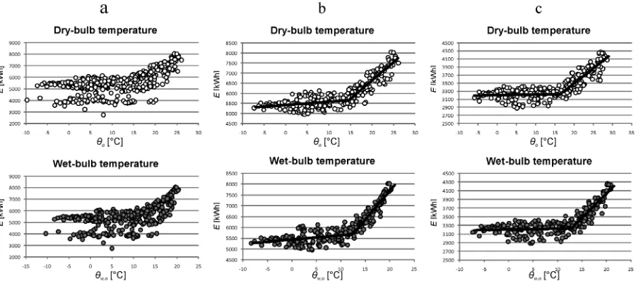
The energy signature method was used first. Initially all available data (i.e. daily electric energy consumption and mean daily temperature) were used to plot the dry-bulb and wet-bulb energy signature. Both of the resulting energy signatures indicated the existence of two energy consumption levels as shown in Fig. 5a. Since this was clearly the consequence of occupancy variation, the non-working days (weekends and holydays) were filtered out and the base temperatures were determined with piecewise linear regression from the energy signatures reploted with the filtered data (Fig. 5b). The thus obtained regression lines on the left side of base values had noticeably positive slopes, which was not in accordance with the theory of the energy signature method. By definition the left side of energy signatures is weather independent, so the regression lines should have been parallel to the temperature axis (zero slope). A detailed analysis of hourly data revealed that the root cause of this deviation lies in the use of building overall electric energy consumption. The problem is that space cooling is not the only contributor to energy consumption, thus changes in operation of building systems and equipment whose energy consumption

represents the base load, i.e. the non-weather related energy consumption, also influence the determination of base temperatures. In our case the reduction of night-time ventilation rate in winter resulted in considerably lower energy consumption in days in which the HVAC system operated under the winter regime compared to the days when space cooling was off and the ventilation rate was not dropped. For this reason, the building base load seemed to increase with temperature.

In order to eliminate the influence of base load variation, hours outside the working schedule (7 a.m. to 5 p.m.) were removed from the working day data. The so filtered data was then used to plot the energy signatures for a third time and to calculate the dry-bulb and wet-bulb base temperature (Fig. 5c). All the base values obtained from the energy signature method are listed in Table 1.

Table 1. Base temperatures determined using the energy signature method

Working days Working days 7 a.m. to 5 p.m.

R2 _R2

θb [°C] 14.6 0.84 16.4 0.78

θw,b [°C] 12.4 0.88 12.8 0.83

Next, the performance line method was applied. Each base temperature was determined twice, once with degree days calculated from daily averaged hourly dry-bulb/wet-bulb temperature differences (Eq. (3)) and once with daily differences (Eq. (4)) as shown in Fig. 6. The results are listed in Table 2.

Base temperatures determined using hourly values are higher than those determined with daily values, which can be explained with the fact that hours are too small time increments to capture the thermal storage effect. In contrast, the wet-bulb base values are almost equal. The reason for this is very simple and lies in the meteorological data. The outdoor wet-bulb temperature varies little throughout the day compared to the dry-bulb temperature (Fig. 7), therefore the mean daily wet-bulb temperature differs very little from individual hourly values, i.e. the daily standard deviation of wet-bulb temperature is small.

Table 2. Base temperatures determined using the performance line method

Hourly values Daily values

θb[°C] 21.5 16.1

θw,b [°C] 12.4 12.1

In comparison with base temperatures determined via energy signature method from filtered workday data (7 a.m. to 5 p.m.), the base values obtained from performance lines using daily temperature differences (Eq. (4)) are slightly lower. The differences are due to the chosen time interval for base temperature determination from energy signatures. Because the lowest temperatures of a day occur at the filtered out hours, the mean temperatures calculated for the selected averaging period are higher than the mean daily temperatures, hence the energy signatures and with them the base temperatures are shifted forward on the temperature axis. As a result monthly dry-bulb

and wet-bulb cooling degree days (Table 3) were calculated only for base temperatures determined via performance lines using daily values. Whereby degree days were calculated only with the calculation procedure, which was employed in determination of base values (i.e. mean daily temperature method).

Fig. 7. Daily progress of dry-bulb and wet-bulb outdoor temperature on July 23rd_{, 2009}

Although the annual sums of dry-bulb and wet-bulb cooling degree days differ marginally, the differences between degree days totals for transitional months are up to 123% (October percentage difference in relation to CDD).

To find out which cooling degree day method is more accurate, performance lines were constructed (linear regression) from monthly total electric energy consumption and each set of monthly degree day data (Fig. 8), and predictions of monthly energy consumptions were made using the performance lines equations (Table 4). The predicted monthly consumptions were then compared against actual consumptions:

∆E E E

E

p a

a

% %,

( )

where ΔE is the percentage difference between actual and predicted monthly electric energy consumption,

Ep is the predicted monthly energy consumption and

Ea is the actual monthly energy consumption.

As seen in Fig. 9 the wet-bulb cooling degree method better predicted energy consumption for three of five months during the cooling season and for eight months overall. The dry-bulb cooling degree method had smaller prediction errors for June and August (besides for November and December), whereby the predicted values were 0.7 % for June and 0.1 % for August more accurate as the values predicted with the

CDDw method. The biggest difference was between the energy consumptions predicted for September, where consumption predicted with the CDDw performance line was 5.9 % closer to the actual energy consumption. While February energy consumption was most underestimated as a consequence of that February has the least number of days, consumptions for October and November were most overrated by both performance lines. In comparison with May, the cooling degree values (dry-bulb and wet-bulb) for October were significantly lower, but the total electric energy was higher. It was similar for November, i.e. total energy consumption in November was considerably higher than in other months with zero degree days. Both of these deviations can be explained by base load modification.

4 CONCLUSSION

Cooling degree days are the summation of temperature differences between the outside air and a reference

temperature over time, and can be applied to estimate future building energy consumption due to space cooling or to monitor energy performance of existing buildings. Although the cooling degree day method is superior to other simplified methods for analysing weather related energy consumption in buildings, because CDD capture both the extremity and duration

Fig. 8. Performance line; a) constructed with CDD, b) constructed with CDDw

Table 3. Monthly dry-bulb and wet-bulb cooling degree days calculated to θb = 16.1 °C and θw,b = 12.1 °C

Month CDD [K·day] CDDw[K·day]

Feb. 09 0 0

Mar. 09 0 0

Apr. 09 0 0

May 09 84 62

Jun. 09 82 82

Jul. 09 162 156

Aug. 09 188 175

Sept. 09 44 74

Oct. 09 10 22

Nov. 09 0 0

Dec. 09 0 0

Jan. 10 0 0

Σ 570 571

Table 4. Predicted and actual monthly total electric energy consumption

Month _CDD Ep [kWh] _CDD Ea[kWh] w

Feb. 09 152977 151385 135646

Mar. 09 152977 151385 151042 Apr. 09 152977 151385 147405 May 09 180737 173977 169512

Jun. 09 179896 181215 179470 Jul. 09 206370 207874 207498 Aug. 09 215007 214845 215859 Sept. 09 167578 178185 178365

Oct. 09 156167 159210 172636

Nov. 09 152977 151385 160653

Dec. 09 152977 151385 153638

Jan. 10 152977 151385 151896

of outdoor temperatures, there are several issues in the application of degree days to cooling energy use in buildings. A key issue, apart from selecting a calculation procedure for degree days, is the definition of a proper base temperature, because the building’s balance point varies together with heat gains and the indoor temperature. However, the main problem lies in the definition of CDD method itself, since it neglects the influence of latent cooling loads on cooling energy, as a consequence from being derived from the heating degree day (HDD) method.

In this article an improved cooling degree method the so-called wet-bulb cooling degree method, which takes into account both the sensible and latent loads, is used to analyse electric energy consumption data from an existing building and compared against the conventional cooling degree day approach, whereby different degree day calculation techniques and statistical methods for determining base temperature are applied.

The results of the analysis are unambiguous, i.e. the CDDw method outperformed the CDD method in the majority of cases. Not only was the correlation between CDDw and electric energy consumption considerably higher (5% higher explained variance), but it was also revealed that the value of wet-bulb base temperature is less dependent on the method chosen for determination (energy signature and performance line method) and on the used degree day calculation procedure (daily averaged hourly and daily temperature differences). Nevertheless, the results obtained by any of the tested methods should be interpreted carefully when dealing with energy consumption data consisting of weather related and non-related energy consumption (i.e. total energy consumption).

In spite of the fact that the wet-bulb cooling degree approach performed well on the selected total electric energy consumption data, it will have to be additionally tested on the data obtained from other existing buildings with different types of air-conditioning systems, preferably on chiller power consumption data.

5 NOMENCLATURE

List of symbols:

CDD Cooling degree days [K·day]

E Total electric energy consumption [kWh]

ELD Enthalpy latent days [kJ/kg·day]

h Specific enthalpy of air [kJ/kg]

HDD Heating degree days [K·day]

t Time [day]

x Absolute humidity of air [kg/kg]

θ Temperature of air [°C]

List of abbreviations:

a Actual b Base d Day m Month o Outdoor p Predicted w Wet-bulb 6 REFERENCES

[1] Košir, M., Krainer A., Dovjak M., Rudolf, P., Kristl, Ž. (2010). Alternative to the Conventional Heating and Cooling Systems in Public Buildings. Strojniški vestnik – Journal of Mechanical Engineering, vol. 56, no. 9, p. 575-583.

[2] Day, A.R., Knight, I., Dunn, G., Gaddas, R. (2003). Improved methods for evaluating base temperature for use in building energy performance lines. Building Service Engineering Research & Technology, vol. 24, no. 4, p. 221-228, DOI:10.1191/0143624403bt073oa. [3] Huang, Y.J., Ritschard, R., Bull, J., Chang, L. (1986).

Climatic indicators for estimating residential heating

and cooling loads. Report LBL-21101. Lawrence

Berkley Laboratory, Berkley.

[4] Krese, G., Prek, M., Butala, V. (2011). Incorporation of latent loads into the cooling degree days concept.

Energy and building, vol. 43, no. 7, p. 1757-1764, DOI:10.1016/j.enbuild.2011.03.042.

[5] ASHRAE (2009). Handbook – fundamentals (SI).

American Society of Heating, Refrigerating and Air-Conditioning Engineers, Atlanta.

[6] Hitchin, E.R. (1983). Estimating monthly

degree days. Building Service Engineering

Research & Technology, vol. 4, no. 4, p. 159, DOI:10.1177/014362448300400404.

[7] Day, A.R., Maidment, G.G., Ratcliffe, M.S. (2000). Cooling degree-days and their applicability to building

energy estimation. 20:20 Vision: CIBSE/ASHRAE

Conference.

[8] Jacobsen, F.R. (1985). Energy signature and energy monitoring in building energy management systems.

Proceeding of CLIMA 2000 World Congress, vol. 3: Energy Management, p. 25-31.

[9] Guan, L. (2009). Preparation of future weather data to study the impact of climate change on buildings.