Study of Adaptive Model Parameter Estimation for Milling Tool Wear

(1)

*Corr. Author’s Address: Lanzhou Polytechnic College, Qilihequ, Gongjiawan 1, 568

Study of Adaptive Model Parameter Estimation for Milling

Tool Wear

Xu, C. ‒ Xu, T. ‒ Zhu, Q. ‒ Zhang, H.

Chuangwen Xu1,*_{‒ Ting Xu}2_{‒ Qi Zhu}1_{‒ Hongyan Zhang}1 1 _{Lanzhou Polytechnic College, China}

2 _{School of Electronic Engineering, Jilin University, China}

In a modern machining system, tool wear monitoring systems are needed to get higher quality production. In precision machining processes, especially surface quality of the manufactured part can be related to tool wear. This increases industrial interest for in-process tool wear monitoring systems. For the modern unmanned manufacturing process, an integrated system composed of sensors, signal processing interface and intelligent decision making model are required. In this study, a new method for on-line tool wear monitoring is presented under varying cutting conditions. The proposed method uses wear feature extraction based on process modeling and parameter estimation. An adaptive estimation model of milling tool wear in variable cutting parameters is built based entirely on milling power. The adaptive model traces the properties of cutting process by combining process state signal, cutting conditions, power model. The tool wear feature is obtained from the estimated parameters of the model and carried on in the theoretical and experimental study. Experiment results have proved that changes of the parameters in the cutting power model significantly indicate tool wear independently of varying cutting conditions and it makes tool wear a recognized process with high precision.

Keywords: milling power, adaptive estimation model, tool wear, model parameters, information fusion

0 INTRODUCTION

Metal-cutting tool wear directly affects the precision, efficiency and cost efficiency of machining, so the on-line monitoring tool wear is becoming increasinhgly important, and has become an important research topic of flexible manufacturing system engineering. With other mechanical processing methods, the milling mechanism is more complex, while condition diversity, cutting parameters variability, and tool breakage and wear is random and complex. Thus, the feature extraction of milling tool wear is the key in tool wear monitoring research. This can effectively resolve the problem directly related to the accuracy and reliablity of milling tool wear monitoring. Therefore, new monitoring theories and technologies have been developed to solve the feature extraction of tool wear. In the previous literature [1] to [5], the identification method regarding the milling tool wear conditions is to identify the main purpose of tool wear, which reached a stage, and then a different processing method is applied according to the different

phases. But in the automated production, the conditions of tool wear can be identified, and tool wear value must be also obtained to satisfy the machining accuracy through compensating the tool radius and optimizing the cutting parameters in time. In this study, the research method to obtain tool wear value is presented. In the tool wear process, tool wear occurs as a process concerned with time, which requires the monitoring system to identify current tool wear value at any time, so as to provide a basis for compensating tool wear.

(2)

source signals, it is not easy to extract the feature information of tool wear from complex signals in time-domain, frequency-domain. In addition, many past methods were developed to monitor tool wear by measuring spindle and feed motor power (current) and proved that the tool wear is very sensitive to the change of the cutting power [9] and [10]. In the cutting process, techniques for tool wear monitoring are being used widely using the spindle and feed motor power. It does not interfere with cutting process by measurement equipment and the machine tool was not formed by a reworking process. However, generation mechanisms of the milling tool wear are more complex and in the view of various factors that affect tool wear, it is difficult to build the exact practical analysis model. Therefore, it is necessary to use experimental data to ensure the analysis and model. In some general methods, an explicit model is built by using Multivariate Linear Regression analysis method [11] and [12] or an implicit model by using the Neural Network [13]. MLR method for monitoring tool wear by measuring spindle and feed motor power is to establish a mathematical model between milling cutting parameters and the classification by fuzzy pattern using MLR analysis. Then, tool wear model for spindle and feed motor power is established. Tool wear value is predicted by tool wear model. Tool wear model is adjusted using cutting parameters to give it better dynamic, fuzzy and real-time characteristics. Therefore, it will be effective to be used in the nonlinear predictive control systems. The NN method for monitoring tool wear by measuring spindle and feed motor power is to establish a Neural Network model which contains milling cutting parameters and cutting power. Then, tool wear network model is trained by using several experimental data of tool wear in different cutting process. Tool wear value is predicted by the Network model. Several problems exist with these methods; (1) It is diffcult to establish an exact practical analysis model between milling cutting parameters and tool wear. (2) The model based on spindle and feed motor power is used to recognize tool wear and can also cause larger error in a different cutting process by using the MLR method because tool wear model coefficients are fixed, that is, of low-precision and limiting applications. (3) The results of prediction are

usually unstable because it is difficult to overcome multicollinearity of variables using the MLR method. (4) NN is difficult to give a reasonable interpretation of the factors influencing tool wear model.

In flexible manufacturing systems, varying cutting conditions are a great challenge to reliable wear monitoring. Intelligent monitoring strategies currently dominate in research work. Intelligent monitoring includes machining processes, signal sensing, feature extraction, learning/ recognition, decision making and control. The performance of the whole monitoring system is heavily dependent upon the effectiveness of the feature extraction. The strategies for wear feature extraction in developed monitoring systems may be summarized in two categories based on the techniques for signal processing and analysis. A pattern recognition method is employed to identify tool wear based on various features. The parametric method includes two stages. In stage one; an empirical model is developed by regression analysis of experimental data. In stage two, tool wear is estimated in real-time using the empirical model and measurements of the cutting state signal and conditions. The advantage of the parametric method is that cutting conditions are used as a model input, so that wear estimation is independent of variation in the cutting condition. In actual machining, the empirical model still has large errors in the estimated tool wear or errors in recognition [14].

An improved strategy is proposed in this study for tool wear monitoring to solve such problems faced in the nonparametric and the parametric methods.

1 TOOL WEAR SENSING BASED ON PROCESS MODELLING AND PARAMETER

ESTIMATION

1.1 Strategy

(3)

During machining, tool wear will create an error between the measured signal and the model output. The model then adjusts its parameters to eliminate the error. Therefore, changes in model parameters indicate tool wear. The wear feature extraction method is independent of variations of the cutting conditions. In step two, tool wear recognition, variations of the features obtained in step one are used to estimate or classify the tool wear state. Several empirical models, which describe the quantitative relationship between the features and actual wear are developed for wear estimation. Some innovative models, in which the learning and classifying functions are performed simultaneously by self-learning, are also developed for tool wear classifications [14].

1.2 Process Modelling and Parameter Estimation Techniques

For processes with specified input and output variables, models can be expressed mathematically as static and dynamic. Static process models usually use nonlinear polynomials, while dynamic process models use differential equations. For processes with only output variables, such as vibrations in machining processes, an autoregressive moving averaging (ARMA) model is suitable. Time-varying models are used for tine-varying processes. A process model may be derived from either a theoretical analysis or from an empirical formula. The well-known least squares (LS) method is normally used for parameter estimation. With on-line monitoring, a recursive LS method should be adopted. The primary advantage of the parameter estimation method is for multiple fault detection.

1.3 LS Method

The least square method - a very popular technique - is used to compute estimations of parameters and to fit data. It is one of the oldest techniques of modern statistics as it was first published in 1805 by the French mathematician Legendre in a now classic memoir. But this method is even older because it turned out that, after the publication of Legendre’s memoir, Gauss, the famous German mathematician, published another memoir (in 1809) in which he mentioned that he

had previously discovered this method and used it as early as 1795. A somewhat bitter anteriority dispute followed (a little reminiscent of the Leibniz-Newton controversy about the invention of Calculus), which, however, did not diminish the popularity of this technique. Galton used it (in 1886) in his work on the heritability of size, which laid down the foundations of correlation and (also gave the name) regression analysis. Both, Pearson and Fisher, who did so much in the early development of statistics, used and developed it in different contexts (factor analysis for Pearson and experimental design for Fisher).

Functional fit example: regression. The oldest (and still most frequent) use of OLS was linear regression, which corresponds to the problem of finding a line (or curve) that best fits a set of data. In the standard formulation, a set of pairs of observations is used to find a function giving the value of the dependent variable from the values of an independent variable. With one variable and a linear function, the prediction is given by the following equation:

Y a bX= + . (1)

This equation involves two free parameters which specify the intercept (a) and the slope (b) of the regression line. The least square method defines the estimate of these parameters as the values which minimize the sum of the squares (hence the name least squares) between the measurements and the model (i.e., the predicted values). This amounts to minimizing the Eq:

ε=

∑

(

Y Yi− i

)

=

∑

Yi−

(

a bX+ i

)

i

 2 _[ _{] ,}2 ₍₂₎

(where ε stands for “error” which is the quantity to be minimized). This is achieved using standard techniques from calculus, namely the property that a quadratic (i.e., with a square) formula reaches its minimum value when its derivatives vanish. Taking the derivative of ε with respect to a and b

and setting them to zero gives the following set of Eqs. (called the normal equations):

∂

∂ = +

∑

−

∑

=

ε

a 2Na 2b Xi 2 Yi 0, (3)

∂

∂ =

∑

+

∑

−

∑

=

ε

(4)

Solving these two Eqs. gives the least square estimates of a and b as:

a M= Y +bMX, (5)

with MY and MX denoting the means of X and Y

and:

b Y M X M

X M

i Y i X

i X

=

(

−

)

(

−

)

−

(

)

∑

2 . (6)

OLS can be extended to more than one independent variable (using matrix algebra) and to non-linear functions.

Multiple Regression Least Square Method. The term multiple regression originates from a multiple number of independent variables (control parameters), which means that the dependent variable is changed by more than one independent variable. The examples of fitting equations are as follows:

• Two independent variable: Z=aA+bB+c (where Z: dependent variable; A, B: independent variables; a, b, c: constants). • Three independent variable: Z=aA+bB+cC+d

(where Z: dependent variable; A, B, C: independent variables; a, b, c, d: constants).

Let us think about the multiple regression with two independent variables to simplify the situation. The least square error in multiple regression will be:

ε = _ −

(

)

_{ =} = _ −

(

+ +

)

_ = =

∑

Z f x y

Z a bx cy

i i i

i n

i i i

i n , . 2 1 2 1 (7)

The first derivatives of ε in terms of a and

b will be (Eqs. 8 to 10):

∂

∂ =

∑

₌  −

(

+ +

)

 =

ε

a _i Zi a bx cyi i

n

2 0

1

, (8)

∂

∂ =

∑

₌  −

(

+ +

)

 =

ε

b _i x Zi i a bx cyi i

n

2 0

1

, (9)

∂

∂ =

∑

₌  −

(

+ +

)

 =

ε

c _i y Zi i a bx cyi i

n

2 2 0

1

. (10)

The Eqs. expended from Eqs. (8) to (10) will be:

Zi a b x c y

i n i n i i n i i n = + + = =

∑

= =

∑

1

∑

1

1 1 1

, (11)

x Z_{i i} a x b x c x y

i n i i n i i n i i n i = + + = = = =

∑

1 1 2 1 1

, (12)

y Z_{i i} a y b y c y

i n i i n i i n i i n = + + = = = =

∑

1 1 1

2

1

. (13)

Computation of the unknown constants using A_{= }X X X Y



−

T 1 T _{and matrices will be} (Eq. (14)).

If you have a data set (x1,y1,Z1), (x2,y2,Z2), ..., (xn,yn,Zn), computations of unknowns (a,b,c)

are computed using matrices.

2 PARAMETER ESTIMATION METHOD FOR TOOL WEAR

In the milling process, the cutting power P

is of the relation with the cutting speed, the feed speed f, the cutting depth ap and the cutting tool

wear VB. At the same time, the cutting power changes with the different conditions such as the part material, the tool material and so on.

a b c

x y

x x x y

i n i i n i i n i i n i i n i i i n           = = = = = = =

∑ ∑

∑

∑ ∑ ∑

1

1 1 1

1

2 1 1

yy y y

x i i n i i n i i n i n i i n = = = = =

∑ ∑

∑

                      1 1 2 1 1 1 1 T

∑

∑ ∑ ∑

∑ ∑

∑

= = = = = = =    y

x x x y

y y y

i i n i i n i i n i i i n i i n i i n i i n 1 1 2 1 1 1 1 2 1                                          − = =

∑

1 1 1 1 i n i i n x

∑

∑ ∑ ∑

∑ ∑

∑

= = = = = = =    y

x x x y

y y y

i i n i i n i i n i i i n i i n i i n i i n 1 1 2 1 1 1 1 2 1                                = = =

∑

T Z x Z y Z i i n i i i n i i i n 1 1 1                                

(5)

According to the metal-cutting principle, the spindle cutting power and the feed power are defined as follows [15] and [16]:

P a v f as = 1 a2 a3 pa4, (15)

P_f b v f ab b p b

= ₁ 2 3 4, (16)

where a1 and b1 are the coefficients determined by the cutting tool geometry dimension and performance of the material. a2, a3, a4 and b2, b3,

b4 is the exponent of the cutting parameters.

As Eqs. (15) and (16) show, a corresponding power value is output under certain cutting conditions and the cutting tool wear states. Eqs. (15) and (16) are a static nonlinear. The Eqs. can be written in the form as:

lnP_s =lna a₁+ ₂lnv a+ ₃lnf a+ ₄ln ,a_p (17)

lnPf =lnb b1+ 2lnv b+ 3ln f b+ 4ln .ap (18)

If S = lnPs, F = lnPf, then:

S a a= ₁+ ₂lnv a+ ₃ln f a+ ₄ln ,a_p (19)

F b b= +1 2lnv b+ 3ln f b+ 4ln .ap (20)

Where XT_{= [1, ln}_v_{, ln}_f_{, ln}_a_p_],

A = [a2, a2, a3, a4]T, B = [b2, b2, b3, b4]T. XT is parameter matrix, A and B is coefficient matrix.

A series of milling states in varying cutting conditions are measured as follows:

Y_i ={ , ,v f a S F_i _i _pi, , },_i _i (21)

Where Yi is corresponding processing

states under different cutting conditions, Pi is

spindle cutting power, vi is cutting speed, fi is feed

speed and api is cutting depth.

For these process states, Eqs. (19) and (20) can be written as:

S i( )=X i A e iT( ) + ( ), (22)

F i( )=X i B e iT( ) + ( ),₍₂₃₎

where e is the model error.

The parameters estimated by the Least Square Method (Eqs. (7) to (14)) are:

A a a a a

_{= } 



1, , ,2 3 4 T, (24)

B_{= }b b b b 1, , ,2 3 4_ .

T

(25)

In real-time tool wear monitoring, the parameter estimation is confirmed by the recursive least square method according to the model error function.

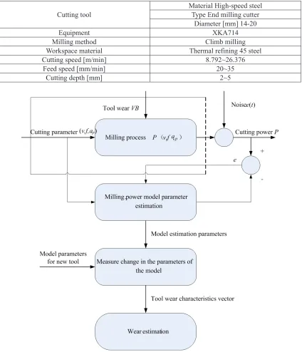
The wear feature extraction strategy using cutting power modeling and parameter estimation is shown in Fig. 1. The procedure is summarized as follows:

a) Establish a process model which describes the relationship between cutting conditions and cutting power, i.e. Eqs. (15) and (16). b) Use sensors to measure the model inputs and

outputs (e.g. speed and power).

c) Estimate the model parameters using the Least Square Method. Detect changes in the model parameters as tool wear increase. These changes are stored as the wear feature parameter.

d) Recognize tool wear by estimating or classifying tool wear based on the wear feature [14].

3 THE TIME-VARIANT CHARACTERISTIC OF PARAMETERS ON POWER MODEL

Experiments are conducted in a XKA714 using the strategy described above. The milling experimental condition is shown in Table 1. Cutting experiment is used in a new tool (VB = 0.05 mm), respectively, according to the first, second and third group of cutting parameters in Table 2, consisting of 48 cutting group parameters by orthogonal combination. At the same time, spindle power and feed power value are detected. Input and output data for 48 group model are obtained. Eqs. (22) and (23) are used to fit the experimental data by the least square method and the results are shown in Tables 3 and 4. A worn tool (VB = 0.25 mm) is used to repeat these experiments and the results are shown in Tables 5 and 6.

(6)

From experimental data in Tables 3 to 6 it can be seen that in normal cutting circumstances (the new cutting tool), the fitting error for 16, 32 and 48 groups of experimental data is all less than 3.5%, and that model parameter estimation

on three batches of data is very similar. From model results of tool wear it follows that the three groups of estimated model parameters are very similar and model fitting error is less than 6.5. The model parameters have a relatively fixed value

Table 1. Cutting experiment condition

Cutting tool Material High-speed steelType End milling cutter Diameter [mm] 14-20

Equipment XKA714

Milling method Climb milling

Workspace material Thermal refining 45 steel

Cutting speed [m/min] 8.792~26.376

Feed speed [mm/min] 20~35

Cutting depth [mm] 2~5

(7)

Table 2. The experimental groups of the cutting parameters (Notes: v [m·min-1_{], f [mm·r}-1_{], a}_p_[mm])

Level _v The first group_F _a The second group The third group

p v F ap v F ap

1 8.792 3.0 5 9.671 3.0 4 13.19 3.0 4

2 9.671 2.5 4.5 11.43 2.5 3.75 15.38 2.5 3.75

3 11.43 2.0 3.5 13.19 2.0 3 21.96 2.0 3

4 13.19 3.0 3 15.38 3.0 2.75 26.376 3.0 2.75

Table 3. The parameter estimation results of the spindle cutting power model (VB = 0.05 mm)

a1 a2 a3 a4 _{error [%]}Fitting The first group data estimation 7.1021 0.1056 0.1734 0.0786 2.46 The first and second group data estimation 7.1471 0.1174 0.1637 0.0777 2.78 First, second and third group data estimation 7.1802 0.1057 0.1745 0.0796 3.12

Table 4. The parameter estimation results of the feed power model (VB = 0.05 mm)

b1 b2 b3 b4 _{error [%]}Fitting The first group data estimation 5.1021 0.2056 0.1734 0.0786 2.38 The first and second group data estimation 5.2862 0.2157 0.1839 0.0795 2.62 First, second and third group data estimation 5.1326 0.2305 0.1879 0.0736 3.04

Table 5. The parameter estimation results of the spindle cutting power model (VB = 0.25 mm)

a1 a2 a3 a4 _{error [%]}Fitting The first group data estimation 9.1602 0.1752 0.1854 0.0886 3.76 The first and second group data estimation 9.1674 0.1875 0.1837 0.0857 4.75 First, second and third group data estimation 9.1803 0.1887 0.1897 0.0897 6.42

Table 6. The parameter estimation results of the feed power model (VB = 0.25 mm)

b1 b2 b3 b4 _{error [%]}Fitting The first group data estimation 6.1328 0.2359 0.1854 0.0778 4.47 The first and second group data estimation 6.2872 0.2212 0.1897 0.0891 5.73 First, second and third group data estimation 6.3352 0.2418 0.1872 0.0932 5.18

Table 7. Selection on cutting speed and feed speed

Cutting parameters ₁ ₂ ₃ ₄ Group number₅ ₆ ₇ ₈ ₉

v [m·min-1_] _8.792 _13.2 _{17.584 21.98 24.178 26.276 28.574 30.772 32.97}

f [mm·r-1_] ₃ _2.75 _2.5 _2.5 ₂ ₂ _1.75 _1.5 ₁

corresponding to tool wear, and this has laid a good foundation for looking for the adaptive of tool wear. Comparing two sets of the experiment, it can be seen that worn tool model parameters

(8)

4 THE FEATURE EXTRACTION OF TOOL WEAR

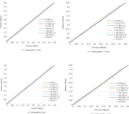
The experiment of tool wear is designed to the varying cutting condition according to round trip milling and multi-feed. The cutting depths during every feed are 3.5, 2, 1.5 and 1 mm. 9 groups of cutting parameters shown in Table 7 are selected as the cutting speed and feed speed.

The feature extraction method for tool wear is to detect the changes ΔA, ΔB of the model estimation parameters which has been wear and the new tool, and calculate the distance function which indirectly reflects changes in the amount of tool wear. Prio to the experiment, the model parameters for the new tool were stored as the base values. The model parameters were then estimated for various worn tools and changes in the parameters were obtained by subtracting the base values from the estimated parameters. The

parameter changes were evaluated using the Distance function.

D A A

a a a a

1 1 0

1 2 2 2 3 2 4 2

= − =

= + + +

(∆ ) (∆ ) (∆ ) (∆ ) , (26)

D B B

b b b b

2 1 0

1 2 2 2 3 2 4 2

= −

= + + +

(∆ ) (∆ ) (∆ ) (∆ ) , (27)

where D1 is the calculation distance of the model estimation parameters for spindle cutting power, and D2 is the calculation distance of the model estimation parameters for feed power.

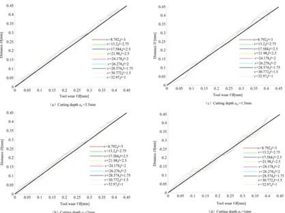
Based on the same cutting depth, in accordance with the cutting parameters of group number in Table 7, the experiment is applied. Eqs. (26) and (27) can be used to calculate the distance. The relationship between distance and tool wear is shown in Figs. 2 and 3. The feature D1, D2 and the

(9)

Table 8. The error statistics between the feature D1 and wear on the spindle cutting power [unit/mm]

Cutting depth ₁ ₂ ₃ ₄Group number₅ ₆ ₇ ₈ ₉

3.5 largest absolute error 0.030 0.020 0.020 0.020 0.030 0.025 0.030 0.025 0.026_{average error} _{0.013 0.015 0.012 0.012 0.014 0.016 0.013 0.013 0.012}

Table 9. The error statistics between the feature D2 and wear on the feed cutting power [unit/mm]

3.5 largest absolute error 0.020 0.021_{average error} _{0.012 0.012 0.012 0.013 0.013 0.014 0.013 0.012 0.015}0.20 0.025 0.025 0.018 0.020 0.020 0.020

Table 10. The error statistics between the distance and the tool wear [unit/mm]

1.5 largest absolute error 0.029 0.023 0.025 0.027 0.027 0.027_{average error} _{0.013 0.013 0.014 0.018 0.018 0.014 0.012 0.017 0.017}0.03 0.024 0.029

error statistics of tool wear are shown in Tables 8 and 9.

From Table 8, feature and statistical error of tool wear for the spindle cutting power can be seen: in the whole tracking tool wear, the largest absolute error is below 0.03 mm, and the average error is equal to 0.017 mm; from Table 9, feature and statistical error of tool wear on the feed cutting power can be seen: in the whole tracking tool wear, the largest absolute error is below 0.025 mm, and the average error is equal to 0.015 mm. It can be seen: (1) identification method for adaptive

(10)

identification differences in tool wear of the spindle power and feed power, feature distance function is used in two types of fusion based on the cutting spindle power and feed power. The two weights respectively 0.4 and 0.6 are satisfactory according to the experiment results.

D A A B B

a a a a

= − + − =

=

( )

+

( )

+

( )

+

( )

0 4 0 6

0 4

1 0 1 0

1 2 2 2 3 2 4

. .

.

∆ ∆ ∆ ∆ 22

1 2 2 2 3 2 4 2

0 6

+

+ . (∆b ) +(∆b ) +(∆b ) +(∆b ) .

(28)

According to Table 7, the experiment is applied to the group number in the same depth. Table 10 can be used to calculate the error

statistics between the feature distance and the tool wear, and its result is shown in Table 10.

Compared to Table 10 and Table 8, Table 9, the fusion distance function of tool wear feature can track the changes of tool wear value well and accurately; average error is 0.014 mm and the largest absolute error is less than before during tool wear identification.

5 CONCLUSION

(11)

processing parameters, processing state is predicted by using power model and least squares estimate model parameters. Model parameters are corrected according to the forecast error, so that the model automatically adapts to track the properties of the cutting process and obtains the parameters of the model as tool wear feature to achieve tool wear monitoring. The experiment results have shown that the model coefficients can be processed with the adaptive changes of processing conditions, and wear value is accurately estimated by feature parameter. In the actual processing, in order to achieve the different types of intelligent tool wear monitoring, this study can be used for tool wear feature extraction methods of different types of processing cutting power model parameters of self-learning.

6 ACKNOWLEDGEMENT

This research was supported by the Natural Science Foundation of Gansu under the research grant 1010RYZA173. The authors thank Cheng Zhongwen from CAD/CAM for providing super alloy material, and also Zhao Youxin, Liu Xiaobin and Li Baodong for their support.

7 REFERENCES

[1] Xu, C.W. (2009). Condition monitoring of milling tool wear based on fractal dimension of vibration signals. Strojniški vestnik ‒ Journal of Mechanical Engineering, vol. 55, no. 1, p. 15-25.

[2] Xu, C.W. (2009). Milling tool wear forecast based on the partial least-squares regression analysis. Structural Engineering and Mechanics, vol. 31, no. 1, p. 1-19.

[3] Wang, Y.L. (2008). Detection of the tool wear condition based on the computer image processing. Journal of Key Engineering Materials, vol. 375, no. 1, p. 553-557. [4] Al-Azmi, A. (2009). Rapid design of

tool-wear condition monitoring systems for turning processes using novelty detection.

Journal of Manufacturing Technology and Management, vol. 17, no. 3, p. 232-245. [5] Cuneyt, A. (2009). Tool wear condition

monitoring using a sensor fusion model based on fuzzy inference system.

Mechanical Systems and Signal Processing, vol. 23, no. 2, p. 539-546.

[6] Mannan, M.A., Kassim, A. (2000). Application of image and sound analysis techniques to monitor the condition of cutting tools. Journal of Pattern Recognition Letters, vol. 21, no. 11, p. 969-979.

[7] Dimla, D.E. (2002). The correlation of vibration signal features to cutting tool wear in a metal turning operation. Journal of Materials Processing Technology, vol. 19, no. 10, p. 705-713.

[8] Srinivasa, P. (2002). Acoustic emission analysis for tool wear monitoring in face milling. Journal of Production Research,

vol. 40, no. 5, p. 1081-1093.

[9] Shao, H., Wang, H.L. (2004). A cutting power model for tool wear monitoring in milling. Journal of Machine Tools and Manufacture, vol. 44, no. 14, p. 1503-1509. [10] Ertunc, M.H., Loparo, A.K. (2001). Tool

wear condition monitoring in drilling operations using hidden Markov models (HMPs). Journal of Machine Tools and Manufacture, vol. 41, no. 9, p. 1363-1384. [11] Chen, J.C. (2004). A multiple-regression

model for monitoring tool wear with a dynamometer in milling operations. Journal of Technology Studies, vol. 30, no. 4, p. 71-77.

[12] Xu,C.G., Wang, X.Y. (2006). New approach on monitoring cutting tool states by motor current. Journal of Instrument Technique and Sensor, vol. 32, no. 4, p. 34-40.

[13] Palanisamy, P., Rajendran, I. (2007). Prediction of tool wear using regression and ANN models in end-milling operation.

Journal of Advanced Manufacturing Technology, p. 1433-3015.

[14] Wan, J. (1996). Intelligent tool failure monitoring for machining processes.

Tsinghua Science and Technology, vol. 1, no. 2, p. 172-175.

[15] Lu, J. (2005). Theory of metal cutting. China Machine Press, Beijing, p. 123-132.