in the population sciences published by the Max Planck Institute for Demographic Research Konrad-Zuse Str. 1, D-18057 Rostock · GERMANY www.demographic-research.org
DEMOGRAPHIC RESEARCH
VOLUME 26, ARTICLE 21, PAGES 543-592
PUBLISHED 08 JUNE 2012
http://www.demographic-research.org/Volumes/Vol26/21/ DOI: 10.4054/DemRes.2012.26.21
Research Article
The temporal dynamics of international
migration in Europe: Recent trends
Jack DeWaard
James Raymer
© 2012 Jack DeWaard & James Raymer.
This open-access work is published under the terms of the Creative Commons Attribution NonCommercial License 2.0 Germany, which permits use, reproduction & distribution in any medium for non-commercial purposes, provided the original author(s) and source are given credit.
1 Introduction 544
2 Background 545
3 Data and methods 547
4 Results 553
4.1 Foreign-born population stocks and migration rates 553 4.2 The expected duration of residence of international migration 557 4.2.1 Summarizing the expected duration of residence for receiving
countries 569
4.2.2 Heterogeneity by citizenship and age 571
4.3 Summary 574
5 Discussion and conclusion 575
6 Acknowledgements 576
References 577
The temporal dynamics of international migration in Europe:
Recent trends
Jack DeWaard1
James Raymer2
Abstract
Descriptive studies of international migration typically rely on measures of migrant stocks and migration rates to assess migration patterns. In this paper we propose a third alternative. Using harmonized data on age-specific migration flows between all countries in the European Union (EU) and European Free Trade Association (EFTA) each year from 2002 to 2007, we estimate the expected duration of residence of international migration, defined as the average number of years lived by migrants in the receiving country given period migration and mortality schedules. Our results provide a window into the temporal dynamics of international migration in Europe, increasingly relevant given recent expansions of the EU.
1 Department of Sociology, Center for Demography and Ecology, University of Wisconsin-Madison, 8128
William H. Sewell Hall, 1180 Observatory Drive, Madison, WI 53706. E-mail: [email protected].
1. Introduction
In this paper we provide estimates of the average time lived by international migrants in each of 31 countries in the European Union (EU) and European Free Trade Association (EFTA) from 2002 to 2007. Though termed the “waiting time” of migration by Palloni (2001:265), we prefer the term, the ‘expected duration of residence’,3 to emphasize our
attention to migration (as opposed to, but not excluding, mortality) and to distinguish the measure developed here from those typically used to summarize international migration, i.e., foreign-born population stocks and migration rates. International migration is a dynamic process characterized by variable time lived in sending and receiving countries, expectations which are largely dependent on the age-structure of migration flows. We argue that a measure summarizing these temporal dynamics at the level of sending and receiving countries should be standard fare in descriptive accounts of international migration patterns.
Few efforts have examined the temporal dynamics of international migration at the country-level. The dearth of data on duration of stay has resulted in analyses largely confined to single-country surveys (Klinthäll 2001; Reagan and Olsen 2000; Waldorf 1994; Waldorf and Esparza 1991), which are inadequate for tracking transitions between each and every pair of sending and receiving countries, and counts of persons and person-years required to take a multistate approach to his issue.4 Moreover, while
published sending and receiving countries’ reports of international migration flows are freely available from statistical agencies such as Eurostat, these lack a common metric across countries, preventing analysts from combining these data in any meaningful way (Kupiszewska and Nowok 2008; Poulain, Perrin and Singleton 2006).
Our efforts take advantage of recently harmonized, i.e., consistent in definition, estimates of age-specific, country-to-country migration flows for 31 countries in the EU/EFTA each year from 2002 to 2007. These were developed as part of the MIgration MOdelling for Statistical Analysis (MIMOSA) project (de Beer et al. 2010; Raymer, de Beer and van der Erf 2011), which combined both sending and receiving countries’ reports of international migration flows, along with covariate information, to arrive at a consistent and complete set of estimates. These estimates represent a significant improvement relative to published sending and receiving countries’ reports, which are marred by inconsistencies in data collection, measurement, and availability (Poulain, Perrin and Singleton 2006). They are also the largest harmonized data source on migration flows between countries in the world. Finally, since they are benchmarked to
3 We are grateful for the comments and suggestions of Alberto Palloni and two anonymous reviewers. 4 The terms “multistate” (Schoen 1988) and “multiregional” (Rogers 1975, 1995) are viewed here as
a one-year timing criterion, these estimates align with the United Nations’ (1998) recommendations for measuring international migration.
With mortality data, we use the MIMOSA estimates to construct period increment-decrement life tables each year from 2002 to 2007. These track the age-specific transitions of persons via migration and death to arrive at a measure which summarizes the expected duration of residence of international migration, i.e., the average number of years lived by migrants in the receiving country given period migration and mortality schedules. A conditional life expectancy at birth, this measure summarizes the average number of years lived in the receiving country j beyond age zero given prior residence in country i at age zero (Willekens and Rogers 1978). Just as life expectancy at birth is often used to summarize the mortality conditions of countries with respect to the age structure of death, the expected duration of residence developed here is viewed as capturing the context of migrant reception and incorporation in receiving countries with respect to the age structure of migration and death.
2. Background
Descriptive studies of country-level patterns of international migration place almost exclusive reliance on measures which summarize in different ways the volume of migration. Foreign-born population stocks refer to the size or concentration of foreign-born persons relative to the total population in receiving countries, while migration rates express recent departures (emigration), arrivals (immigration), or the balance of the two (net-migration). Although each is necessary to understand international migration patterns, they are not exhaustive.
Individual-level studies have shown that the amount of time lived by migrants in receiving areas serves an integrative and to a lesser extent equalizing role where migrants’ labor market and mobility outcomes are concerned (Adsera and Chiswick 2007; Redstone and Massey 2004; Borjas, Bronars and Trejo 1992). Migrants’ time lived in receiving areas has likewise been linked to reductions in individual prejudice on the part of natives given more potential opportunities for constructive interpersonal contacts with foreigners (Allport 1954; Pettigrew 1998; Pettigrew and Meertens 1995; Schneider 2008; Schlueter and Scheepers 2010). For example, in his analysis of internal migration within the United States, Alexander (2005:654) noted that a “highly transient migrant stream can inhibit the development of [a] migrant community…and draw at least some sort of antipathy from both long-term settlers and other local residents alike.”
understanding of migration patterns and the effects on social exclusion. Pitkin and Myers (2011:258, emphasis ours) recently argued that while many “empirical studies have yielded a multitude of specific” findings, the result has been “a plethora of disjointed and inconsistent results that yield little information about the overall [trend].” To date, the character and utility of a summary measure of the temporal dynamics of international migration that compliments stock- and rate-based measures is unknown. This is unfortunate from a migration policy perspective, where both the reception and incorporation of migrants in receiving countries is often implicit (Huddleston et al. 2011).
One possible reason for the inattention to the temporal dynamics of international migration lies in the substantial data requirements, and the fact that sending and receiving countries’ reports of international migration flows are incomparable in their publicly available forms. As we detail in Section 3 of this paper, the measure for the expected duration of residence of international migration developed here is generated from dynamic population models which require a single matrix of age-specific migration flows between all pairs of sending and receiving countries each year.
Publicly available migration data in Europe consist of both emigration and immigration counts. However, when particular flows between countries are compared, these reports are frequently inconsistent (Kupiszewska and Nowok 2008:43-45). These inconsistencies arise because there is no common metric used to measure migration across countries. First, there is no consensus on what exactly constitutes a valid transition. For example, whereas migrations constitute events, migrants are persons who have undergone a change in status from non-migrant. Cross-national analyses therefore suffer from differing national viewpoints concerning exactly what or who is a migration or migrant, respectively. Second, migration is seldom measured directly, and is often inferred as a change in residence in a population register, or by comparing place of residence at two points in time. Compounding these issues is the fact that countries use different methods of data collection (Poulain, Perrin and Singleton 2006:222-227), which include administrative records, decennial population censuses, or surveys. Timing criteria likewise vary considerably across countries, and may refer to persons who plan to live or have lived in a different country for no specified period of time, three months, six months, one year, or permanently.
have large enough sample sizes to capture the level of detail required to analyze country-to-country migration flows without severe irregularities in the data. In some instances reported flows for certain countries may be missing for particular years or altogether. Migration data may also be available only for the total population and not for more detailed demographic, socioeconomic, or spatially disaggregated subgroups required for targeted studies.
Because of these problems only limited work has been carried out in the area of estimating international migration flow matrices. There is, however, at least one major exception that focuses on European migration. The estimates produced by the MIMOSA project, as described in de Beer et al. (2010) and Raymer, de Beer and van der Erf (2011), represent the first set of flows that are truly amenable to cross-national comparison at a relatively large scale.5 We use these harmonized estimates of
international migrant stocks and migration flows for 31 countries in the EU/EFTA each year from 2002 to 2007 in the current project.
3. Data and methods
We use multistate methods (Rogers 1975, 1995; Schoen 1988) to construct period increment-decrement life tables which track the age-specific transitions of international migrants from and to 31 countries in the EU/EFTA, a residual “rest of the world” category, and to death each year from 2002 to 2007. The state-space is thus comprised of 33 states and is exhaustive.6 The total number of transitions analyzed in this project
is thus 114,048.7
Data requirements include, for each year, age-specific country-to-country transition rates. As stated in the introduction, we use harmonized estimates of age-specific country-to-country migration flows from and to all countries in the EU/EFTA (including from and to the rest of the world) each year from 2002 to 2007, obtained from the MIMOSA project. The methodology used to produce these estimates is described in de Beer et al. (2010) and Raymer, de Beer and van der Erf (2011), and the estimates themselves are available at the Netherlands Interdisciplinary Demographic Institute’s website.8 Based on a hierarchical procedure, available country-to-country
migration flow data were harmonized using the reports of sending and receiving
5 Another example currently in progress is the Integrated Modeling of European Migration (IMEM) project
(Raymer et al. 2010).
6 The term state refers to any of the 31 EU/EFTA countries, the “rest of the world” as a single entity, or death. 7 We track 1,056 transitions between 32 sending states (not including death) and 33 receiving states
(including death, which is absorbing) for 18, five-year age groups each year from 2002 to 2007, totaling 1,056 * 18 * 6 = 114,048 possible transitions.
countries following an extension of Poulain’s (1993, 1999) optimization procedure. Missing marginal and origin-destination associations were then estimated using a multiplicative component approach and incorporating covariate information. The estimated origin-destination-specific flows were then disaggregated by age and sex based on patterns exhibited by countries with available data.
With respect to the remaining data requirements, the MIMOSA project also provides harmonized age-specific population counts for each year (Kupiszewska, Wiśniowski and Bijak 2009). Annual population counts for the rest of the world were obtained by subtracting the former counts for countries in the EU/EFTA from age-specific estimates of the global population for each year obtained from the U.S. Census’ International Database (IDB). Annual age-specific death counts were obtained for EU/EFTA countries from Eurostat’s New Cronos database and, for the rest of the world, by subtracting the former counts for EU/EFTA countries from the number of deaths estimated for each year from global model life tables available from the World Health Organization (WHO).9
Our conceptual model is presented in Figure 1. The state-space depicted is a first-order Markov process where, for country i, qij and qji represent country-to-country
transition probabilities at each age, and qid and qjd represent the force of mortality
(Palloni 2001; Rogers 1975, 1995; Schoen 1988).
Figure 1: Model of states and transitions
9 Given that global model life tables from the WHO are available for 2000 and 2008, we linearly interpolate
Toward estimating each of the probabilities in Figure 1, the starting point for constructing increment-decrement life tables is to assemble age-specific transition matrices of migration rates, M(x), each year (Palloni 2001; Schoen 1988). For a system comprised of k countries, these matrices take the form:10
⎤ ⎢ ⎢ ⎢ ⎢ ⎡ − − − − − −
∑
∑
2 2 2 21 1 1 12 1 L L d x n k x n j j x n x n d x n k x n x n j j x n M M M M M M M M emig ⎥ ⎥ ⎥ ⎥ ⎥ ⎥ ⎦ ⎢ ⎢ ⎢ ⎢ ⎢ ⎢ ⎣ − − − =∑
0 0 0 0 2 1 L L M M O M M kd x n j kj x n k x n k xnM M M M
(x)
Μ (1)
Excluding the last row and column, each of the rows and columns in (1) represent sending and receiving countries, respectively. The off-diagonal elements are the rates of
⎥ ⎥ ⎥ ⎥
ration from each country i to j between ages x and x+n, multiplied by negative one. Each diagonal element represents the sum of the emigration rates from country i to any and all receiving countries (j = 1, 2,…, k for i≠j) and death. Transitions from and to death are accommodated by setting the elements in the last row to zero, and those in the last column to the age-specific death rate in the sending country,
−
nMxid (i = 1, 2,…,k).
Life table construction is carried out by converting each of the rates in (1) into probabilities and tra
expo
cking age-specific transitions at each age. With occurrence-sure rates this can be done using Schoen’s (1988) general algorithm or, alternatively, Rogers’ (1995:96) “Option 1” method (Rogers and Ledent 1976), each with the assumption that the transitions from country i to j are linear in the age interval x to x+n (Palloni 2001):
l(x+n) = l(x)[I - 2.5M(x)][I + 2.5M(x)]-1 (2)
10 Noting that sending and receiving countries represent columns and rows, respectively, the equivalent
notation in Rogers (1995:96; see also Rogers and Ledent 1976), where deaths are embedded along the main diagonal, is:
⎥ ⎤ ⎢
⎡ +∑ − − k
x n x n j j x n d x
nM M M L M
nal elements are counts of those who did not migr
ature (Preston, Heuveline and Guillot 2001; Rogers 1995). Lastly, I is an identity matrix, while the M(x) matrix is the same as that discussed above. Summing each column in the l(x+n) matrix and arranging these totals along the main diagonal, with zero
yields the l(y) matrix (not shown).12 In the subsequent age interval this matrix then
takes the place of the l(x) matrix to repeat the calculation in (2) until each age interval is en be asse bled into a multistate life table.
Because the MIMOSA dat
calen ar years from 2002 to 2007, it is necessary to transform the rates in (1) at the
king a tra
The l(x+n) matrix contains counts of migrants and non-migrants at the end of the age interval x to x+n. The off-diagonal elements are counts of completed transitions from country i to j, while the diago
ate. The l(x) matrix contains along the main diagonal, with zeros in the off-diagonal elements, the number of survivors at age x. At age zero these values represent the size of the hypothetical birth cohort in each country. Here, to minimize the potentially distorting impact of population size across countries (Herting et al. 1997), these values are set equal, as is convention in the liter
11
s in the off-diagonal elements,
exhausted. This iterative process yields a set of components which can th m
a are available in five-year age intervals for single d
outset so that these reflect the probability of transition over five years, 5qxij. This is
achieved with the following transformation, derived from the probability of not ma nsition in a single year, raised to the power of five:13
5
5 5
5 1 1 1 0.5
⎥ ⎥ ⎦ ⎤ ⎢ ⎢ ⎣ ⎡ ⎟⎟ ⎠ ⎞ ⎜⎜ ⎝ ⎛ + − − = ij x ij x ij x M M
q (3)
Working directly with the probabilities derived in (3), equation (2) reduces to:
l(x+n) = l(x)Q(x) (4)
where Q(x) is a matrix of age-specific transition probabilities, wherein each row is a probability vector, arranged in exactly the same way as the migration rates in (1).
sk. A primary innovation in this project is the number of states (n=33) considered to comprise the state-space. Multistate demographic programs, e.g., SPACE (Rogers 1995; see also Willekens and
Constructing period increment-decrement life tables is a cumbersome though not intrinsically difficult ta
Rogers 1978), are available and user
11 All radixes are set to 100,000.
12 See Schoen (1988) and Palloni (2001). Rogers’ (1975, 1995; see also Rogers and Ledent 1976) method
achieves the same result, but tracks transitions from country i to j using the columns of the l(x+n) matrix, thereby requiring summation across the rows to generate the l(y) matrix.
;
a
friendly however, the maximum number of states is limited to four. While other options are available without these restrictions, e.g., C++ program developed by Tiemeyer and Ulmer (1991) and, more recently, LIPRO developed by van Imhoff and Keilman (1991; see also van Imhoff 2005 and Willekens 2011), we followed Palloni’s suggestion (2001:272) and developed a routine for increment-decrement life table construction using the Stata statistical software package. This provided greater control in implementing the above solutions and estimating the key quantities of interest in this project detailed below.
The key quantities of interest in this project are a set of period, conditional life expectancies at birth:
i ij ij T
e = 0 (5)
l0
where Tij
0 is the total number of person-years lived in country j above age zero by those
with prior residence in country i at exact age zero, and li
0 is the size of the hypothetical
birth cohort in country i at exact age zero (Willekens and Rogers 1978). When i≠j, this quantity summarizes the “waiting time” of international migration for each and every pair of sending and receiving countries (Palloni 2001:265). Alternatively, when i=j, this quantity expresses these dynamics for non-movers. As mentioned earlier, we refer to the quantity in (5) as the expected duration of residence, to stress the contribution of migration to their construction and interpretation. It is important to recognize that this measure summarizes the cumulative effects of age-specific, country-to-country migration, including both emigration and immigration. Although the data are unavailable r in
0
fo ternational migration, it would be preferable to further condition on coun y of birth (Ledent 1981; Philipov and Rogers 1981; Rogers and Belanger 1990; Roge nd Raymer 2005).
he above quantities are standard in the multistate liter
1975, 1995; Schoen 1988), where one conditions on a single sending country, e, and then estimates the average years that a person could be expected to live in each and every receiving country. From the
this means that a set of measures, one for each sending country i (i = 1, 2,…, k for i≠j), describe the temporal dynamics of international migration. However, to obtain a single summary measure for each receiving country that can be compared against more
com u
tr rs a
T ature (see Palloni 2001;
Rogers one at a tim
perspective of the receiving country,
sending countries) could be expected to live in the receiving country above age zero, denoted by e*j
0 :
j i w e
e k ij
i ij
j =
∑
≠= , 0 1 0 *
0 , (6)
where j i n n w k i ij ij
ij = ≠
∑
=
total migration (counts) from country i to j. If one were to arra h of the quantities in (5) into a matrix, where each element is the expected idence lived in country j beyond age zero by persons previously residing exact age zero, then it is clear that the quantity in (6) is just a weighted average of expected durations of residence across all sending countries (i = 1, 2,…, k tive of the receiving country is not standard in the multistate literature (Palloni 2001), these relationships are
the temporal dynamics of international migration by taking into account the migration linkages shared by specific pairs of sending and
,
1
0 . (7)
Note, nijdenotes
nge eac durat n of res in country i at
io
for i≠j) for each receiving country. Although taking the perspec
nonetheless embedded in the mechanics of multistate life tables.14 We further wish to
consider the very different likelihoods and sizes of migration to each receiving country,
ij
w0 , which vary substantially depending on the sending country. The quantity in (6) thus accounts for the relative size of migration from each sending country and thereby provides an average picture of
14 Let the superscript ⌐j denote any country but j. The expected duration of residence in country j for persons
from any sending country but j is then:
j
≠ (8)
When li
0 is constant across sending countries, equation (8) simplifies to an average of the expected durations
of residence across all sending countries.
i l T l T e k i i k i ij j jj jj= =
∑
∑
= = ¬ ¬ ¬ , 1 0 1 0 0 0 0 ji≠ (9)
For ease of notation and because we apply weights after the fact, we adopt the notation in equation (6) to denote that the expected duration of residence is a weighted average for the reasons discussed above. Nonetheless, we detail equations (8) and (9) to demonstrate that there is nothing inherent in the mechanics of multistate life tables which prohibits one from taking the perspective of the receiving country.
l T k e k i i ij jj=
∑
= ¬ 1 ,
1 0
recei
ign-born population stocks are presented in Table 1. These were estimated as part of the MIMOSA project (Kupiszewska, Wiśniowski and Bijak 2009). As one might expect, the core immigrant receiving countries in Northern, Western, and Southern Europe have sizeable concentrations of migrants (Castles and Miller 2003). For example, Lichtenstein, Luxembourg, and Switzerland exhibit the largest percentages of foreign-born population stocks at 37%, 34%and 22%, respectively, in 2007. In total, 16 countries in 2007 had foreign-born populations greater than 10% of the total population, including three of the five largest countries in Europe, i.e., France, Germany, and Spain. The countries with the smallest percentages were mostly new EU accession countries, including Bulgaria, Romania, Poland, and Hungary. With a few exceptions, foreign-born population stocks increased from 2002 to 2007. The most sizeable increases over the period were in Spain (+5.36 percentage points), Ireland (+3.56), Iceland (+3.48) and Italy (+2.19). In contrast, the largest declines were in Latvia (-1.93) and Estonia (-1.73). Overall, the picture is one of increasing concentrations of foreign-born persons over the period, excluding some of the new EU accession countries in Central and Eastern Europe.
ving countries. To illustrate, according to the 2007 MIMOSA estimates, over 75% of migration from countries in the EU/EFTA to the Czech Republic originated in Slovakia. Without the weights, the impact of this important migration exchange would be underrepresented.
4. Results
4.1 Foreign-born population stocks and migration rates
We begin this section by summarizing two measures of international migration, foreign-born population stocks and migration rates, for 31 countries in the EU/EFTA from 2002 to 2007. Since much descriptive work on international migration relies extensively on these measures, our consideration of them here provides a point of comparison and departure in the current paper.
Table 1: Foreign-born population stocks as a percent of the total population in 31 EU/EFTA countries, 2002-2007
Country 2002 2003 2004 2005 2006 2007
AT- Austria 12.75 13.17 13.57 13.98 14.38 14.80 BE- Belgium 10.79 11.12 11.40 11.68 12.07 12.51 BG- Bulgaria 0.55 0.55 0.54 0.54 0.53 0.53 CH- Switzerland 21.42 21.59 21.75 21.90 22.04 22.19 CY- Cyprus 12.81 13.06 13.34 13.63 13.90 14.12 CZ- Czech Republic 4.47 4.45 4.43 4.42 4.40 4.38 DE- Germany 12.81 12.89 12.71 12.84 12.85 12.84 DK- Denmark 7.29 7.47 7.59 7.69 7.84 8.04 EE- Estonia 17.98 17.65 17.31 16.97 16.62 16.25 ES- Spain 6.20 7.73 8.55 9.90 11.26 11.56 FI- Finland 2.79 2.92 3.04 3.18 3.36 3.56 FR- France 10.36 10.53 10.70 10.85 10.85 10.85 GR- Greece 10.36 10.47 10.58 10.68 10.79 10.89 HU- Hungary 2.82 2.77 2.72 2.68 2.63 2.58 IE- Ireland 10.37 9.10 8.91 9.88 14.67 13.93 IS- Iceland 6.40 6.61 6.72 7.04 8.23 9.88 IT- Italy 4.02 4.46 4.91 5.35 5.78 6.21 LI- Liechtenstein 38.81 38.43 38.03 37.68 37.31 36.93 LT- Lithuania 6.10 6.36 6.89 6.61 6.61 6.56 LU- Luxembourg 32.72 33.03 33.35 33.64 33.96 34.27 LV- Latvia 18.04 17.24 16.96 16.65 16.34 16.11 MT- Malta 5.55 5.69 5.83 5.96 6.06 6.04 NL- Netherlands 10.40 10.59 10.65 10.65 10.62 10.59 NO- Norway 6.96 7.33 7.59 7.84 8.20 8.65 PL- Poland 2.08 2.01 1.94 1.88 1.81 1.75 PT- Portugal 6.40 6.53 6.66 6.78 6.89 7.00 RO- Romania 0.61 0.62 0.62 0.62 0.63 0.64 SE- Sweden 11.54 11.78 12.01 12.21 12.44 12.90 SI- Slovenia 10.89 10.92 11.00 10.87 11.10 11.31 SK- Slovakia 2.83 3.49 4.14 4.05 4.15 4.31 UK- United Kingdom 8.40 8.50 8.83 9.26 9.96 9.97
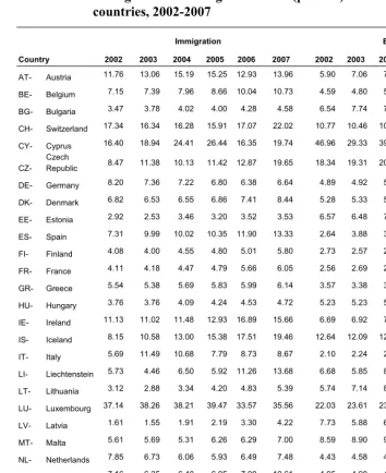
Foreign-born population stocks obscure the distinction between past and recent migrants. To isolate more recent trends we present the estimated rates of immigration and emigration from 2002 to 2007 for the same set of 31 countries in the EU/EFTA. As in Table 1, the flows used to construct these rates were obtained from reports produced by the MIMOSA project (de Beer et al. 2010; Raymer, de Beer and van der Erf 2011). In Table 2 we see that there is a large amount of heterogeneity in the estimated rates of immigration and emigration, though the patterns appear to be relatively stable over time. The highest rates tend to be associated with small countries such as Cyprus and Luxembourg, with a few exceptions such as the immigration rates for Slovenia and Estonia.
Table 2: Immigration and emigration rates (per 000) to/from 31 EU/EFTA countries, 2002-2007
Immigration Emigration
Country 2002 2003 2004 2005 2006 2007 2002 2003 2004 2005 2006 2007
AT- Austria 11.76 13.06 15.19 15.25 12.93 13.96 5.90 7.06 7.65 8.26 9.43 9.73 BE- Belgium 7.15 7.39 7.96 8.66 10.04 10.73 4.59 4.80 5.04 5.30 5.84 6.15 BG- Bulgaria 3.47 3.78 4.02 4.00 4.28 4.58 6.54 7.74 7.89 7.82 8.65 11.54 CH- Switzerland 17.34 16.34 16.28 15.91 17.07 22.02 10.77 10.46 10.79 11.03 11.79 11.97 CY- Cyprus 16.40 18.94 24.41 26.44 16.35 19.74 46.96 29.33 39.79 58.99 41.27 64.53
CZ- Czech
Republic 8.47 11.38 10.13 11.42 12.87 19.65 18.34 19.31 20.00 15.02 20.11 13.01 DE- Germany 8.20 7.36 7.22 6.80 6.38 6.64 4.89 4.92 5.46 5.24 5.42 6.05 DK- Denmark 6.82 6.53 6.55 6.86 7.41 8.44 5.28 5.33 5.63 5.76 6.08 5.78 EE- Estonia 2.92 2.53 3.46 3.20 3.52 3.53 6.57 6.48 7.32 7.53 8.36 8.77 ES- Spain 7.31 9.99 10.02 10.35 11.90 13.33 2.64 3.88 3.48 3.98 7.21 10.85 FI- Finland 4.08 4.00 4.55 4.80 5.01 5.80 2.73 2.57 2.85 2.63 2.62 2.71 FR- France 4.11 4.18 4.47 4.79 5.66 6.05 2.56 2.69 2.88 3.08 3.44 3.61 GR- Greece 5.54 5.38 5.69 5.83 5.99 6.14 3.57 3.38 3.42 3.46 3.43 3.59 HU- Hungary 3.76 3.76 4.09 4.24 4.53 4.72 5.23 5.23 5.88 6.48 7.07 7.56 IE- Ireland 11.13 11.02 11.48 12.93 16.89 15.66 6.69 6.92 7.73 8.16 9.23 9.95 IS- Iceland 8.15 10.58 13.00 15.38 17.51 19.46 12.64 12.09 12.93 12.79 13.45 14.56 IT- Italy 5.69 11.49 10.68 7.79 8.73 8.67 2.10 2.24 2.10 2.16 2.11 2.22 LI- Liechtenstein 5.73 4.46 6.50 5.92 11.26 13.68 6.68 5.85 8.25 7.69 7.82 8.67 LT- Lithuania 3.12 2.88 3.34 4.20 4.83 5.39 5.74 7.14 8.39 8.74 8.20 8.70 LU- Luxembourg 37.14 38.26 38.21 39.47 33.57 35.56 22.03 23.61 23.86 25.29 23.10 25.70 LV- Latvia 1.61 1.55 1.91 2.19 3.30 4.22 7.73 5.88 6.88 6.25 11.03 9.02 MT- Malta 5.61 5.69 5.31 6.26 6.29 7.00 8.59 8.90 9.35 9.50 10.83 10.60 NL- Netherlands 7.85 6.73 6.06 5.93 6.49 7.48 4.43 4.58 4.95 5.44 5.87 6.02 NO- Norway 7.16 6.35 6.40 6.95 7.90 10.61 4.95 4.90 4.66 4.40 4.58 4.55 PL- Poland 2.82 3.01 4.07 4.01 4.63 6.43 6.00 6.16 7.18 8.06 10.91 9.89 PT- Portugal 4.44 4.48 4.69 4.95 5.68 6.02 4.04 4.25 4.39 4.49 4.95 5.32 RO- Romania 2.86 3.17 3.29 3.52 4.00 4.63 8.57 13.27 12.84 12.01 13.53 15.14 SE- Sweden 7.16 7.06 6.85 7.18 10.53 10.87 3.66 3.86 4.09 4.29 4.76 4.86 SI- Slovenia 3.50 2.87 3.51 3.65 3.42 3.58 2.85 2.61 2.93 2.63 2.78 3.30 SK- Slovakia 2.94 3.31 5.70 12.06 16.15 11.01 9.86 10.62 11.57 14.57 15.70 15.98
UK- United
Kingdom 7.16 7.95 9.52 9.07 9.60 9.49 4.58 4.75 4.72 4.94 5.50 5.08
4.2 The expected duration of residence of international migration
The above results generate little in the way of new findings. Northern, Western, and Southern Europe continue to experience unprecedented volumes of international migration into the twenty-first century (Castles 2007). What is not understood to date is whether rising volumes of international migration necessarily translate into longer and thus more permanent migrations, or whether international migrants are simply turning over at rates consistent with the figures in Tables 1 and 2.
e
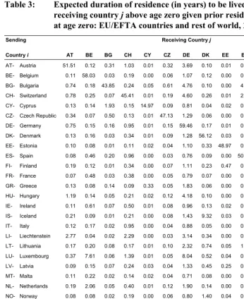
To address this issue, in Table 3 we present a matrix containing the expected durations of residence for each pair of sending and receiving countries in 2007.15 When
summed across each row, these quantities equal total life expectancy at age zero in the sending country, ei∗
0 . Each of the diagonal elements, ii, represent the average number
of years that a person can expect to live beyond age zero in their country of residence at age zero; and the off-diagonal elements, eij
0, represent the average number of years a
person can expect to live in another country j above age zero provided they resided in country i at age zero (for i≠j).
0
16 Note, as stated earlier, that these figures are based on
previous/next country of residence and do not take into account country of birth due to data limitations.
Given the age-specific migration and mortality observed in 2007, persons living in Austria at age zero, for example, could expect to live an average of 75.9 years beyond age zero, of which 51.5 years could be expected to be lived in Austria, 3.7 years in Germany, 8.7 years in other EU/EFTA countries, and 12.0 years outside the EU/EFTA system. By comparison, persons living in Iceland could expect to live an average of 76.6 years above age zero, of which only 39.3 years could be expected to be lived in Iceland. The remaining 37.3 years are divided among 15.8 years in other Scandinavian countries (Denmark, Norway, and Sweden), 3.7 years in the UK, 8.1 years in other EU/EFTA countries, and 9.7 years outside the EU/EFTA system. It is important to note that the quantities in Table 3 should be interpreted as the average number of years for the population across the life course, and not as actual durations of stay for individuals who, in order to be counted as migrants in the estimated data, would have had to stay for at least one year in the country of destination.
The information contained in Table 3 is a valuable source of information on the effects of age- and origin-destination-specific migration. For example, we see that persons living in Norway at age zero can expect to spend, on average, 3.2 years in Sweden. Persons living in Sweden at age zero, on the other hand, can expect to spend
15 These figures are provided for the years 2002-2006 in Appendices 1-3.
16 Had we adopted the mechanics of Rogers (1975, 1995), the figures displayed in Table 3 and in Appendices
s in the Netherlands at age zero living in Belgium, about two years on aver
pectations are between one-half and two-thirds, excluding Luxembourg and yprus.
only 1.9 years in Norway. For flows between the Czech Republic and Slovakia, these differences are even more striking. Persons living in Slovakia at age zero can expect to spend 11.0 years in the Czech Republic, on average, whereas persons living in the Czech Republic at age zero can only expect to spend 1.4 years in Slovakia. In other cases the differences are not as striking. For example, the number of years that persons living in Belgium at age zero can expect to live in the Netherlands is roughly the same as for person
age.
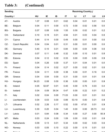
The expected durations of residence in Table 3 can also be used to indicate the retention or “holding power” of countries (Herting, Grusky and Van Rompaey 1997:268). In Table 4 we show the average number of years lived above age zero in country i by those residing in i at age zero each year from 2002 to 2007. Countries are ordered according to the percentage of total life in 2007 lived above age zero in the same country of residence as at age zero. At the top of the list is the “Rest of World” category where, in 2007, persons outside the EU/EFTA system could expect to spend 58.4 years out of a total of 59.2 years (or 98.5%) in this region. The next five countries are Italy (90.9%), Finland (87.2%), Slovenia (86.9%), France (85.6%) and Greece (85.3%). At the bottom of the list are Cyprus (20.6%)17, Luxembourg (38.7%), Iceland
(51.4%), Slovakia (57.6%) and Switzerland (58.9%). In general, persons living in the countries listed in the top half of Table 4 can expect to spend over two-thirds of their lives above age zero in their country of residence at age zero. In the bottom half of the table these ex
C
17 Note, the expectations for Cyprus are particularly low and could reflect an error in the MIMOSA estimates,
Table 3: Expected duration of residence (in years) to be lived by a person in receiving country j above age zero given prior residence in country i
at age zero: EU/EFTA countries and rest of world, 2007
Sending Receiving Country j
Country i AT BE BG CH CY CZ DE DK EE ES FI FR GR
Table 3: (Continued)
Sending Receiving Country j
Country i HU IE IS IT LI LT LU LV MT NL NO
Table 3: (Continued)
Sending Receiving Country j
Country i PL PT RO SE SI SK UK RW
AT- Austria 1.04 0.10 0.99 0.15 0.18 0.44 0.70 12.00 75.94 51.51 24.44 BE-
∑
≠j ij i j e0 ( )
* 0i
e eii
0
Belgium 0.46 0.12 0.07 0.15 0.02 0.05 1.31 7.22 76.52 58.03 18.49 BG- Bulgaria 0.40 0.08 0.57 0.43 0.01 0.26 1.10 10.36 73.48 43.85 29.63 CH- Switzerland 0.69 0.20 0.15 0.40 0.36 0.22 2.68 8.52 77.10 45.41 31.69 CY- Cyprus 0.26 0.03 1.43 0.19 0.00 0.04 3.58 40.65 72.55 14.97 57.58 CZ- Czech Republic 0.22 0.02 0.19 0.07 0.01 1.39 1.21 20.02 73.97 47.13 26.84 DE- Germany 2.86 0.18 0.41 0.21 0.06 0.13 1.01 6.25 76.59 59.46 17.13 DK- Denmark 0.45 0.05 0.06 4.00 0.02 0.09 1.51 6.95 76.03 56.12 19.91 EE- Estonia 0.13 0.02 0.03 1.12 0.00 0.02 2.55 8.03 73.02 48.97 24.05 ES- Spain 0.16 0.57 0.68 0.11 0.01 0.03 1.06 17.04 75.70 50.67 25.03 FI- Finland 0.13 0.02 0.02 1.95 0.01 0.03 0.60 2.40 76.83 66.98 9.85 FR- France 0.28 0.26 0.08 0.08 0.01 0.04 1.18 5.71 77.06 65.95 11.11 GR- Greece 0.45 0.02 0.18 0.24 0.00 0.03 1.36 4.90 76.95 65.60 11.34 HU- Hungary 0.24 0.05 0.50 0.24 0.01 0.39 1.01 8.52 73.16 54.23 18.93 IE- Ireland 1.34 0.13 0.16 0.24 0.02 0.05 3.82 9.74 76.02 52.87 23.15 IS- Iceland 1.66 0.28 0.04 4.03 0.01 0.10 3.74 9.68 76.59 39.34 37.25 IT- Italy 0.31 0.03 0.08 0.06 0.02 0.05 0.46 2.67 78.18 71.03 7.15 LI- Liechtenstein 1.03 0.03 0.07 0.04 0.92 0.04 0.18 8.90 77.34 53.19 24.15 LT- Lithuania 0.73 0.09 0.04 0.87 0.00 0.04 2.44 8.27 71.90 47.81 24.09 LU- Luxembourg 0.67 3.76 0.12 0.50 0.21 0.04 3.55 5.75 76.86 29.73 47.13 LV- Latvia 0.17 0.04 0.02 0.48 0.00 0.03 1.70 12.67 71.19 50.30 20.88 MT- Malta 0.12 0.04 0.03 0.28 0.00 0.06 4.00 16.47 75.54 49.21 26.33 NL- Netherlands 0.58 0.17 0.07 0.27 0.01 0.06 1.60 7.67 76.90 58.92 17.98 NO- Norway 0.58 0.05 0.03 3.18 0.00 0.11 1.45 4.00 77.47 62.57 14.90 PL- Poland 50.43 0.04 0.05 0.57 0.01 0.14 2.82 6.92 74.50 50.43 24.07 PT- Portugal 0.11 60.44 0.06 0.08 0.01 0.02 1.51 5.94 76.53 60.44 16.09 RO- Romania 0.16 0.08 44.31 0.25 0.01 0.35 0.31 8.74 73.96 44.31 29.65 SE- Sweden 0.69 0.04 0.04 61.82 0.03 0.06 1.41 4.99 77.60 61.82 15.78 SI- Slovenia 0.10 0.01 0.02 0.12 66.13 0.16 0.08 3.60 76.09 66.13 9.96 SK- Slovakia 0.28 0.04 0.12 0.11 0.01 42.74 2.34 8.84 74.24 42.74 31.51 UK- United Kingdom 0.38 0.10 0.05 0.20 0.01 0.05 61.65 8.12 76.41 61.65 14.76 RW- Rest of World 0.03 0.01 0.01 0.02 0.00 0.01 0.15 58.37 59.24 58.37 0.87
Source: Authors' calculations
Notes: The expected duration of residence of international migration is a conditional life expectancy at age zero, defined as the average number of years that a person is expected to live in the receiving country j above age zero given prior residence in country i at age zero (Willekens and Rogers 1978; see also Palloni 2001).
= Total life expectancy above age zero in sending country i
* 0i e
= Average number of years a person can expect to live beyond age zero in country i given prior residence in country i at exact age zero
ii e0
= Average number of years a person can expect to live beyond age zero in any country but i given prior residence in country i at exact age zero
∑
j
≠
Table 4: Relative retention times (in years) for 31 EU/EFTA countries and rest of world, 2002-2007
e0ii e0i*
% change in
e0i*
e0ii as % of
e0i*
Country 2002 2003 2004 2005 2006 2007 2007 2002-2007 2007
RW- Rest of World 56.54 56.85 57.20 57.66 58.01 58.37 59.24 3.47 98.53 IT- Italy 70.89 70.32 71.09 71.02 71.35 71.03 78.18 0.96 90.85 FI- Finland 66.49 67.08 66.33 66.99 67.31 66.98 76.83 0.76 87.17 SI- Slovenia 66.87 67.09 66.89 67.98 67.66 66.13 76.09 1.48 86.91 FR- France 68.47 68.20 67.87 67.30 66.32 65.95 77.06 0.93 85.58 GR- Greece 65.80 66.51 66.24 66.20 66.32 65.60 76.95 0.61 85.26 NO- Norway 60.79 61.10 61.98 62.83 62.43 62.57 77.47 1.28 80.76 UK- United Kingdom 62.18 61.98 62.04 61.69 60.26 61.65 76.41 1.13 80.68 SE- Sweden 65.02 64.26 63.72 63.24 62.03 61.82 77.60 0.56 79.67 PT- Portugal 63.29 62.97 62.94 62.56 61.47 60.44 76.53 1.66 78.97 DE- Germany 61.93 61.79 60.18 61.15 61.01 59.46 76.59 1.11 77.64 NL- Netherlands 63.02 62.50 61.58 60.40 59.27 58.92 76.90 1.12 76.61 BE- Belgium 61.69 61.38 60.84 60.14 58.79 58.03 76.52 0.94 75.84 HU- Hungary 57.98 58.48 57.27 56.05 55.26 54.23 73.16 1.53 74.12 DK- Denmark 57.89 57.49 56.62 56.36 55.46 56.12 76.03 1.17 73.82 LV- Latvia 52.13 56.36 55.19 55.28 47.04 50.30 71.19 1.56 70.67 IE- Ireland 58.53 58.39 56.80 56.20 54.29 52.87 76.02 0.89 69.55 LI- Liechtenstein 57.51 60.39 54.17 54.89 55.64 53.19 77.34 1.37 68.77 AT- Austria 60.32 57.41 55.78 55.13 52.19 51.51 75.94 0.16 67.82 PL- Poland 57.84 57.58 55.62 53.97 48.70 50.43 74.50 1.21 67.69 EE- Estonia 52.68 53.35 51.57 51.54 49.88 48.97 73.02 2.59 67.06 ES- Spain 70.29 66.92 67.52 66.13 58.23 50.67 75.70 -1.44 66.94 LT- Lithuania 56.30 52.77 49.67 48.29 49.05 47.81 71.90 0.79 66.49 MT- Malta 53.58 53.64 52.08 51.81 48.89 49.21 75.54 0.29 65.15 CZ- Czech Republic 41.66 39.87 39.68 44.24 38.39 47.13 73.97 1.87 63.72 RO- Romania 50.41 42.46 44.93 47.77 46.14 44.31 73.96 3.37 59.91 BG- Bulgaria 53.47 51.23 50.98 51.04 49.29 43.85 73.48 1.89 59.67 CH- Switzerland 48.43 49.13 48.75 48.29 45.78 45.41 77.10 0.66 58.90 SK- Slovakia 49.39 51.03 49.97 43.86 42.72 42.74 74.24 1.29 57.56 IS- Iceland 43.40 44.59 42.68 43.03 41.45 39.34 76.59 -0.01 51.37 LU- Luxembourg 31.38 29.80 30.12 29.54 32.27 29.73 76.86 1.54 38.68 CY- Cyprus 20.13 28.60 22.13 16.44 21.60 14.97 72.55 0.87 20.64
The information in Table 4 is also useful for examining the effects of EU expansions in 2004 and 2007. Overall, we find that most countries in the EU/EFTA exhibited lower levels of retention in 2007 compared to 2002, suggesting an increase in mobility during this time. Interestingly, these decreases are neither consistent nor apparent across all countries in the system. For example, consider Poland, the largest new EU accession country, which joined in 2004. In 2007 persons at age zero living in Poland could expect to live, on average, 50.4 years of their 74.5 years above age zero in Poland. Between 2002 and 2007 life expectancy in Poland increased by 1.2%; however, the average years lived in Poland above age zero decreased by over seven years over the period. For Bulgaria the corresponding decrease was 9.6 years, most of which occurred in 2007 when Bulgaria joined the EU. Not all decreases, however, represent recent accessions to the EU. People living in Austria at age zero, for example, exhibited a considerable decrease in the average years lived in Austria. In 2002 persons living in Austria at age zero could expect to live 60.3 years above age zero in that country. In 2007 this figure was 51.5 years, a decrease of 8.8 years. In Spain the corresponding drop was nearly 20 years. Increasing foreign populations and return migration could be responsible for some, if not most, of these decreases. The figures for Finland and Norway, on the other hand, increased by one-half of one year and almost two years, respectively. Other countries, such as Greece, Germany, Italy, and the UK remained at about the same levels over the six-year period.
Figure 2: Expected duration of residence (in years) for persons from Poland to EU-15 countries, 2002-2007
0 1 2 3 4 5 6 7 8
AT BE DE DK ES FI FR GR IE IT LU NL PT SE UK
Receiving Country j
e
0
ij
2002 2003 2004 2005 2006 2007
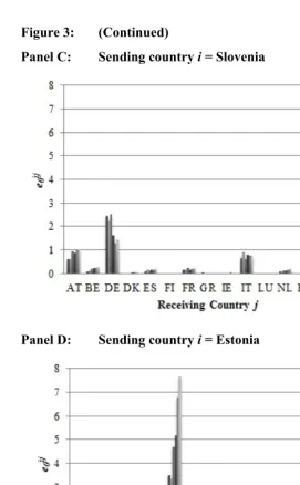
In Figure 3 selected flows from other recent EU accession countries to the EU-15 are presented to illustrate different patterns resulting from our estimates. Here we see that those originating in Bulgaria were more likely to migrate to and reside in Germany and Spain relative to other EU-15 countries. Until 2006 the average number of years lived in Germany had been decreasing. In 2007, however, the number of years lived in Germany more than doubled, from 2.0 years to 4.8 years. Patterns for the Czech Republic and Slovenia were relatively stable over time with no large effects following their accessions to the EU. The number of years that persons originating in Estonia could expect to live in Finland more than doubled between 2002 and 2007, but the patterns for other EU-15 countries, e.g., the UK, remained about the same.
Norway at age zero, the number of years expected to live in Sweden decreased, whereas for persons living in Sweden at age zero, the number of years lived in Finland and Norway trended in the opposite direction.
Figure 3: Expected duration of residence (in years) for persons from selected new accession countries to EU-15 countries, 2002-2007
Panel A: Sending country i = Bulgaria
Figure 3: (Continued)
Panel C: Sending country i = Slovenia
Figure 4: Expected duration of residence (in years) for persons among Nordic countries, 2002-2007
Panel A: Sending country i = Denmark
Figure 4: (Continued)
Panel C: Sending country i = Norway
ma es
While well-kn 01; Rogers 1975, 1995; Schoen
1988), the expected durations of residence as discussed in Section 4.2 provide only a
of the t ra cs of i ati rat use the n
y b rpreted wi sp t e ngl nd try . eve a e
on in ations (6)-(9), one n not co n on gle send
ntry oward e ding th easure described in uation (5 ese n
le r nce or receiving cou ry e E /E
th e Wo n r ea h nation, on tio an an l
in r i These q tities th xpr s verage ber of years
a is expecte j ey e zer ven s
de j, i.e., in an l se din un es 1, 2 r i≠), at age . W ted average pr en for ving country.
igh roportiona he size e m gration flo fr ach sending co ntr
le Expected ati o ide ce ears) w hte y of
migration a d ed by ination: 31 EU rec ivi
countries and rest of rld, 00 7
eivin
4.2.1 Sum rizing the expected duration of residence for receiving countri
own in the multistate literature (Palloni 20
partial picture empo l dynami ntern onal mig ion, beca y ca onl e inte th re ec to th si e se ing coun i How r, s w
dem strated earlier Equ eed nditio a sin ing
cou . Thus, t xten e m Eq ), we pr nt i
Tab 5 the expected durations of eside f each nt in th U FTA and e Rest of th rld, wherei , fo c desti we c di n on y d al send g countries (fo ≠j). uan us e es the a num
that person d to live in receiving country b ond ag o gi previou resi nce outside of y and al n g co tri (i = ,…, k fo j
zero eigh s are es ted each recei As noted earlier, the
we ts are p l to t of th i w om e u y.
Tab 5: dur on f res n (in y eig d b size
flow n summ dest /EFTA e ng
wo 2 2-200
Rec g Country 2002 2003 2004 2005 2006 2007
AT- Austria 0.43 0.48 0.61 0.63 0.61 0.72 BE- Belgium 1.09 1.14 1.18 1.09 1.11 1.07 BG- Bulgaria
erlan 0.68 0.62 0.63 0.64 0.81 us 0.21 0.23 0.20 0.16 0.14
ublic 4.29 3.60 4.31 ny
Liechtenstein 0.00 <0.01 <0.01 <0.01 0.01 0.02
LU-LV- 0.13 0.17 0.23 0.16 0.19 0.48 0.39 0.43 0.45 0.40 0.38 CH- Switz d 0.65
CY- Cypr 0.13
CZ- Czech Rep 3.53 4.23 7.55 DE- Germa 3.01 2.99 3.79 4.28 4.15 4.05 DK- Denmark 0.98 0.92 1.00 0.88 0.85 0.85 EE- Estonia 0.21 0.08 0.23 0.15 0.20 0.21 ES- Spain 2.76 3.56 3.41 3.53 3.76 3.82 FI- Finland 1.06 1.06 1.38 1.54 1.97 2.16 FR- France 1.15 1.14 1.26 1.39 1.40 1.61 GR- Greece 0.81 0.55 0.70 0.98 0.68 1.03 HU- Hungary 0.30 0.30 0.62 0.33 0.37 0.40 IE- Ireland 0.54 0.48 0.49 0.76 0.89 0.73 IS- Iceland 0.17 0.13 0.16 0.19 0.21 0.18 IT- Italy 2.53 6.93 5.60 3.59 4.12 3.99
LI-LT- Lithuania 0.08 0.06 0.06 0.11 0.20 0.23 Luxembourg 0.35 0.35 0.35 0.33 0.27 0.28
Table 5: (Continued)
Receiving Country 2002 2003 2004 2005 2006 2007
MT- Malta 0.01 0.01 0.01 0.02 0.02 0.01 NL- Netherlands 0.49 0.48 0.47 0.49 0.54 0.69 NO- Norway 0.92 0.81 0.69 0.67 0.70 0.89 PL- Poland 1.09 1.16 1.53 1.51 1.51 2.12 PT- Portugal 0.38 0.39 0.44 0.40 0.37 0.47 RO- Romania 0.33 0.33 0.39 0.43 0.46 0.55 SE- Sweden 1.78 1.70 1.41 1.33 1.39 1.31 SI- Slovenia 0.08 0.06 0.06 0.09 0.09 0.15 SK- Slovakia 0.16 0.19 0.25 0.60 0.72 0.56 UK- United Kingdom 1.39 1.59 1.88 1.76 1.81 1.82 RW- Rest of World 9.55 9.50 9.85 9.13 11.02 11.25
Notes: The expected duration of residence in the receiving country is interpreted as the average number of years that a person is ex
terns in Europe.
pected to live in receiving country j above age zero given prior residence outside of country j at age zero (Willekens and Rogers 1978; see also Palloni 2001).
The quantities in Table 5 can be interpreted as follows: using Germany in 2007 as an example, 4.05 is the average number of years that a person is expected to live in Germany above age zero given previous residence in any other EU/EFTA country or the rest of the world at age zero. Recall that the interpretation of this measure assumes constant age-specific migration and mortality schedules prevailing during the period in question, e.g., in 2007. This measure reflects migration at the population level, i.e., the set of all persons exposed to the risk of migration, rather than simply those who happened to migrate during a given period. This explains why some of the estimates, e.g., Lichtenstein, are effectively zero. As weighted averages, these estimates account for the fact that the size of migration flows to a receiving country can and often does differ substantially by the sending country. For example, in 2007, nearly 40% of flows to Germany originated from countries outside of the EU/EFTA (not shown). The corresponding figure for the UK was 67%.
iscrepancies between the volume and temporal dynamics of migration are also evid t among relatively homogenous pairs of countries. While, in Table 2, both
ve rates of net-migration in 2007, of 6.06 and 6.01 per thousand, respectively, the expected duration of residence in Sweden (1.31
Like
ining these types of migration over time, refer to Roge
move, with return migrants exhibiting a slightly older labor force peak. Third, return D
en
Norway and Sweden showed similarly positi
years) is nearly double that of Norway (0.89 years). Likewise, Ireland and the UK, with rates of net-migration in 2007 of 5.71 and 4.41 per thousand, respectively, exhibit differences in the expected durations of residence. The figure for the UK (1.82 years) is more than double that for Ireland (0.73 years). Although there exist extensive literatures on the unique historical, geopolitical, economic, and sociocultural sources of these differences (Castles and Miller 2003; DeWaard, Kim and Raymer forthcoming; Jennissen 2004; Kritz, Lim and Zlotnik 1992; Massey et al. 1998), our aim is more modest and is simply to document discrepancies between the volume and the expected duration of residence of international migration. At present we have fairly strong evidence that these dynamics should be examined concurrently in descriptive accounts of international migration.
4.2.2 Heterogeneity by citizenship and age
many demographic processes, flows of migrants between sending and receiving countries are composed of heterogeneous subpopulations (Vaupel and Yashin 1985). With respect to our estimates, one of the most obvious sources of heterogeneity is migrants leaving and returning to their country of birth. Multistate life tables with this type of origin-dependence were developed and explored for internal migration in the United States by Rogers and Philipov (1979), Ledent (1981) and Philipov and Rogers (1981), and were also detailed by Rogers (1995:140-176). These developments followed earlier analyses, which demonstrated key differences between primary, secondary (or repeat), and return migration using cross-classified U.S. Census data on place-of-residence by place-of-residence-five-years-ago by place-of-birth (Eldridge 1965; Long and Hansen 1977). Primary migrants are those who migrated away from their place of birth. Return migrants are those who migrated to their place of birth. And secondary migrants are those who migrated neither away from nor to their place of birth. For empirical analyses exam
rs and Belanger (1990) and Rogers and Raymer (2005).
nfortunately, consistent and complete birthplace-specific international migration flow tables are unavailable. We therefore have no way to directly test the sensitivity of our results in the presence of return migration to the country of birth. However, toward indirectly exploring this heterogeneity, and thus the Markov assumption, we incorporated age-specific migration data classified by type of citizenship from the MIMOSA project.18 We combined the 2007 estimates of total age-specific emigration
for nationals and foreigners with the corresponding population stocks to obtain age-specific emigration rates for both nationals and foreigners.19 Although not ideal, these
estimates allowed us to test, albeit indirectly, the effects of migrant heterogeneity. We assume that most foreign emigrants are return migrants and most national emigrants are primary migrants. We focus our discussion on the retention expectances (like those in Table 4) for nationals and foreigners, expressed as the percentage of remaining years of life to be lived in country i above ages zero, 20, and 40 given previous residence in i at exact ages zero, 20, and 40, respectively.
migration occurs in both directions. Fourth, the patterns of primary, secondary, and return migration tend to be stable over time. Finally, the retention expectancies, i.e., those who remained in their place of residence, are higher when origin-dependence is included. For example, Rogers and Belanger (1990:204) showed that retention expectancies, expressed in percentages, for birthplace-independent life tables from 1980 U.S. Census data were 53% for New England, 58% for the South Atlantic, 61% for the West South Central, and 41% for the Mountain region. The corresponding retention expectancies from birthplace-dependent life tables were 74%, 83%, 85%, and 72%, respectively.
U
18 Available at http://www.knaw.nl/Pages/NID/24/928.bGFuZz1VSw.html.
19 Bulgaria, Cyprus, Czech Republic, Hungary, Lithuania, Malta, Romania, Slovenia and Slovakia all reported
Table 6: Relative retention times (as percentage of remaining life) for 31 EU/EFTA countries and rest of world by citizenship and age, 2007
All Persons Nationals Foreigners
Country e0ii/ e0i* e20ii/ e20i* e40ii/ e40i* e0ii/ e0i* e20ii/ e20i* e40ii/ e40i* e0ii/ e0i* e20ii/ e20i* e40ii/ e40i*
AT- Austria 67.82 66.52 87.90 86.93 88.85 96.25 24.10 13.86 35.60 BE- Belgium 75.84 75.56 93.58 88.49 90.09 97.43 27.03 18.31 62.92 BG- Bulgaria 59.67 60.10 85.93 80.13 84.28 94.75 26.04 14.72 78.15 CH- Switzerland 58.90 58.74 87.08 75.73 80.38 94.53 31.41 21.41 63.07 CY- Cyprus 20.64 11.93 51.26 83.04 85.97 95.29 28.63 19.92 80.81
CZ- Czech
Republic 63.72 58.60 81.42 97.39 97.62 99.03 29.51 21.02 80.09 DE- Germany 77.64 76.80 91.71 92.52 93.69 97.88 27.61 22.71 43.54 DK- Denmark 73.82 74.88 96.16 82.18 84.78 97.70 26.16 18.29 66.76 EE- Estonia 67.06 68.30 90.27 81.73 84.77 95.13 31.69 24.75 73.85 ES- Spain 66.94 67.14 88.22 91.93 93.73 97.91 19.22 14.78 31.20 FI- Finland 87.17 88.74 97.52 89.03 90.96 97.97 45.81 42.87 73.24 FR- France 85.58 85.27 96.11 93.56 94.30 98.38 43.14 38.19 80.15 GR- Greece 85.26 86.00 96.11 92.83 94.35 98.46 49.44 43.79 65.91 HU- Hungary 74.12 69.96 88.33 96.73 96.90 98.85 26.71 15.94 78.43 IE- Ireland 69.55 68.94 88.57 84.29 85.62 95.12 25.74 25.04 38.47 IS- Iceland 51.37 54.89 93.45 55.73 61.11 93.96 12.43 11.39 70.13 IT- Italy 90.85 92.28 96.89 91.98 93.65 97.02 76.51 74.41 78.22 LI- Liechtenstein 68.77 66.31 92.39 74.62 77.26 92.94 42.62 36.04 80.54 LT- Lithuania 66.49 68.37 90.65 70.40 73.42 92.08 25.85 14.17 77.84 LU- Luxembourg 38.68 36.66 68.86 66.63 76.59 91.71 26.66 18.55 44.75 LV- Latvia 70.67 72.61 86.09 74.85 78.51 88.76 55.73 51.98 75.25 MT- Malta 65.15 63.76 89.91 83.00 85.39 95.86 27.44 17.76 80.30 NL- Netherlands 76.61 79.04 92.83 80.95 84.15 94.72 33.67 32.72 52.17 NO- Norway 80.76 82.22 95.59 89.76 92.14 98.04 24.79 18.68 53.05 PL- Poland 67.69 66.01 88.17 67.37 65.72 88.10 28.67 18.84 79.75 PT- Portugal 78.97 79.95 94.27 90.36 92.42 97.84 19.77 8.58 32.54 RO- Romania 59.91 53.12 79.09 80.55 79.50 91.70 26.67 15.84 78.19 SE- Sweden 79.67 81.69 94.56 86.25 89.13 96.81 32.70 31.31 61.82 SI- Slovenia 86.91 88.84 94.79 93.75 95.74 97.92 26.04 15.07 79.14 SK- Slovakia 57.56 53.07 77.92 72.93 72.93 88.06 27.38 17.13 78.64
UK- United
Kingdom 80.68 80.75 94.23 87.56 88.44 96.42 38.36 36.67 54.58
As expected, our results show that nationals have considerably higher retention expectancies and foreigners have considerably lower retention expectancies than do all migrants combined. For example, persons living in Austria at age zero can expect to spend 67.8% of their lives in Austria. When citizenship is considered, the figure increases to 86.9% for nationals and decreases to 24.1% for foreigners. This pattern is consistent across all countries. Some of the differences between nationals and foreigners, e.g., Spain and Portugal, are particularly large with over 90% retention for nationals and less than 20% for foreigners. For other countries the differences between nationals and foreigners are smaller. For example, Latvia exhibited retention expectancies of 74.9% for nationals and 55.7% for foreigners.
We also found considerable heterogeneity across age. For nationals, the retention expectancies increased as age increased. For example, Luxembourg exhibited retention expectancies of 66.6%, 76.6%, and 91.7% at ages zero, 20, and 40, respectively (see also Iceland). In other cases the differences between ages zero and 20 were not so large. For example, Poland exhibited a retention expectancy of 67.4% at age zero, which decreased slightly to 65.7% at age 20, and then increased dramatically to 88.1% at age 40. For foreigners we find that the retention expectancies are lower for 20 year olds than they are at age zero and at age 40. For example, foreigners in the UK exhibited retention expectancies of 38.4%, 36.7%, and 54.6% at ages zero, 20, and 40 years, respectively. The corresponding figures for France are 43.1%, 38.2%, and 80.2%, respectively.
4.3 Summary
In this section we have shown how different measures of migration provide unique glimpses into patterns of international movement from and to the EU/EFTA, towards both revising and extending current explanations of international migration. The first two measures, foreign-born population stocks and migration rates, are useful for detailing the composition of populations in receiving countries and recent levels of mobility. However, neither of these measures captures the temporal dynamics of international migration produced by the age structure of flows. The expected duration of residence, estimated and extended here, provides an alternative to more conventional measures. Between 2002 and 2007 the EU/EFTA expanded from 19 to 31 countries. Understanding the diverse effects of these expansions is important for considering future expansions, as well as designing policies to deal with issues of increased mobility and the integration of migrants in receiving countries.
considering heterogeneous migration flows and the continued need for [harmonized] data to shed light on these dynamics (Ledent 1981; Philipov and Rogers 1981; Rogers and Belanger 1990; Rogers and Raymer 2005). We hope our work provides a starting point for future efforts aimed at elucidating the inherent diversity of international migration flows by echoing prior calls for cross-nationally comparable data on migrant characteristics (Bell et al. 2002).
5. Discussion and conclusion
We have provided a descriptive account of the expected duration of international migration in 31 countries in the EU/EFTA each year from 2002 to 2007. A core innovation of this project is the use of harmonized estimates of country-to-country migration flow data available from the MIMOSA project. The issues remedied by these data are serious enough to call into question the host of descriptive and empirical works making use of published sending and receiving countries’ reports of international migration, given the lack of a common metric across countries. These data also provide a glimpse into migration patterns from and to countries that fail to report these figures for some or all migration flows.
In 2007 the European Parliament established clear definitions of emigration and immigration. Member states are now required to provide migration flow data to Eurostat (Regulation (EC) No 862 2007). This regulation, however, has not gone far enough to remedy the problem of the incomparability of sending and receiving countries’ reports of international migration flows. In particular, the regulations do not stipulate a precise and uniform set of methods for estimating migration flows, or require countries to alter their systems of data collection (Fassman 2009). Until such conventions are implemented, methods for harmonizing and also estimating missing emigration and immigration reports of sending and receiving countries are necessary to ensure that international migration is measured and modelled consistently across countries.
years. Where issues of international migration intersect with labor market pressures, population aging, and public pensions, it is important that descriptive accounts of country-level migration patterns take into account age-specific migration propensities and the corresponding durations of residence of international migration (Bauer and Zimmerman 1999).
We noted earlier that the measure developed in this project is one way to aid thinking about the context of migrant reception and integration in receiving countries. Migrants who reside in destination countries for longer periods are not necessarily the most highly visible with respect to foreign-born population stocks and migration rates. A large body of theoretical and empirical scholarship has demonstrated positive associations between the proportionate concentration of migrants and various indicators of social exclusion in receiving countries (Blalock 1967; Citrin and Sides 2006; Quillian 1995; Schneider 2008; Semyonov, Raijman and Gorodzeisky 2006). However, little is known about the potential role of the expected duration of residence of international migration at the country-level. Following Ceobanu and Escandell (2010), we suggest that a fruitful extension to the work of this project include empirical efforts to establish or disconfirm the importance of the expected duration of residence as one potential source of cross-country variation in the social exclusion of migrants (see also Pachucki, Pendergrass and Lamont 2007). The efficacy of this measure may yield new insights into societal contexts of migrant reception and incorporation relevant to scholars and policy-makers alike.
6. Acknowledgements
References
Adsera, A. and Chiswick, B.R. (2007). Are there gender and country of origin differences in immigrant labor market outcomes across European destinations? Journal of Population Economics 20(3): 495-526. doi:10.1007/s00148-006-0082-y.
Alexander, J.T. (2005). “They’re never here more than a year:” Return migration in the southern exodus, 1940-1970. Journal of Social History 38(3): 653-671. doi:10.1353/jsh.2005.0039.
Allport, G. (1954). The Nature of Prejudice. New York: Perseus Books Publishing. Bauer, T.K. and Zimmermann, K.F. (1999). Assessment of Possible Migration Pressure
and its Labour Market Impact Following EU Enlargement to Central and Eastern Europe. Bonn: Institute for the Study of Labor (Research Report No. 3).
Bell, M., Blake, M., Boyle, P., Duke-Williams, O., Rees, P., Stillwell, J., and Hugo, G. (2002). Cross-national comparison of internal migration: Issues and measures. Journal of the Royal Statistical Society Series A (Statistics in Society) 165: 435-464. doi:10.1111/1467-985X.00247.
Blalock, H.M. (1967). Toward a theory of minority group relations. New York: Wiley. Bongaarts, J. (2004). Population Aging and the Rising Cost of Public Pensions.
Population Development Review 30(1): 1-23. doi:10.1111/j.1728-4457.2004.000 01.x.
Borjas, G.J., Bronars, S.G. and, Trejo. S.J. (1992). Self-selection and internal migration in the United States. Journal of Urban Economics 32(2): 159-185. doi:10.1016/0094-1190(92)90003-4.
Castles, S. (2007). Twenty-First Century Migration as a Challenge to Sociology. Journal of Ethnic and Migration Studies 33(2): 351-371. doi:10.1080/1369 1830701234491.
Castles, S. and Miller, M. (2003). The Age of Migration: International Population Movements in the Modern World, 3rd edition. New York: The Guilford Press.
Ceobanu, A.M. and Escandell, X. (2010). Comparative analyses of public attitudes toward immigrants and immigration using multinational survey data: A review of theories and research. Annual Review of Sociology 36: 309-328. doi:10.1


![The Scottish economy [February 1986]](data:image/gif;base64,R0lGODlhAQABAIAAAP///wAAACH5BAEAAAAALAAAAAABAAEAAAICRAEAOw==)