in the population sciences published by the Max Planck Institute for Demographic Research Konrad-Zuse Str. 1, D-18057 Rostock · GERMANY www.demographic-research.org
DEMOGRAPHIC RESEARCH
VOLUME 26, ARTICLE 6, PAGES 151-166
PUBLISHED 02 MARCH 2012
http://www.demographic-research.org/Volumes/Vol26/6/ DOI: 10.4054/DemRes.2012.26.6
Research Material
Mapping the results of local statistics:
Using geographically weighted regression
Stephen A. Matthews
Tse-Chuan Yang
This publication is part of the Special Collection on “Spatial Demography”, organized by Guest Editor Stephen A. Matthews.
© 2012 Stephen A. Matthews & Tse-Chuan Yang.
This open-access work is published under the terms of the Creative Commons Attribution NonCommercial License 2.0 Germany, which permits use, reproduction & distribution in any medium for non-commercial purposes, provided the original author(s) and source are given credit.
1 Introduction 152
2 Geographically Weighted Regression (GWR) 153
3 Mapping local GWR results 154
4 Discussion 160
5 Acknowledgements 161
Mapping the results of local statistics:
Using geographically weighted regression
Stephen A. Matthews1
Tse-Chuan Yang2
Abstract
BACKGROUND
The application of geographically weighted regression (GWR) – a local spatial statistical technique used to test for spatial nonstationarity – has grown rapidly in the social, health, and demographic sciences. GWR is a useful exploratory analytical tool that generates a set of location-specific parameter estimates which can be mapped and analysed to provide information on spatial nonstationarity in the relationships between predictors and the outcome variable.
OBJECTIVE
A major challenge to users of GWR methods is how best to present and synthesize the large number of mappable results, specifically the local parameter parameter estimates and local t-values, generated from local GWR models. We offer an elegant solution.
METHODS
This paper introduces a mapping technique to simultaneously display local parameter estimates and local t-values on one map based on the use of data selection and transparency techniques. We integrate GWR software and GIS software package (ArcGIS) and adapt earlier work in cartography on bivariate mapping. We compare traditional mapping strategies (i.e., side-by-side comparison and isoline overlay maps) with our method using an illustration focusing on US county infant mortality data.
CONCLUSIONS
The resultant map design is more elegant than methods used to date. This type of map presentation can facilitate the exploration and interpretation of nonstationarity, focusing map reader attention on the areas of primary interest.
1 Associate Professor of Sociology, Anthropology and Demography, Faculty Director of the Geographic
Information Analysis Core, Population Research Institute, Social Science Research Institute, Pennsylvania State University.
1. Introduction
3Across the sciences there has been a recent emergence of techniques for examining local relationships in data based on analytical approaches that focus on subsets of data (e.g., locally weighted scatterplot smoothing (LOWESS), a technique developed by Cleveland 1979). Techniques for the analysis of local spatial relationships also have recently emerged (for an overview see Lloyd 2011).
The conventional approach to the empirical analyses of spatial data is to calibrate a global model. The term ‘global’ implies that all the spatial data are used to compute a single statistic or equation that is essentially an average of the conditions that exist throughout the study area in which the data have been measured. The underlying assumption in a global model is that the relationships between the predictors and the outcome variable are homogeneous (or stationary) across space. More specifically, the global model assumes that the same stimulusprovokes the same response in all parts of the study region. However, in practice, the relationships between variables might be nonstationary and vary geographically (Cressie 1993; Jones and Hanham 1995). Spatial nonstationarity exists when the same stimulus provokes a different response in different parts of the study region. If nonstationarity exists then there is a suggestion that different processes are at work within the study region.
Standard global modeling techniques, such as ordinary least squares (OLS) linear regression or spatial regression methods, cannot detect nonstationarity and thus their use may obscure regional variation in the relationships between predictors and the outcome variable. Public policy inference based on the results from global models, where nonstationarity is present but not detected, will be variable and may be even quite poor in specific local/regional settings (Ali, Patridge, and Olfert 2007).
Geographically Weighted Regression (GWR) is a statistical technique that allows variations in relationships between predictors and outcome variable over space to be measured within a single modeling framework (Fotheringham, Brunsdon, and Charlton 2002; National Centre for Geocomputation 2009). As an exploratory technique, GWR provides a great richness in the results obtained for any spatial data set, and should be useful across all disciplines in which spatial data are utilized. Indeed, applications of GWR include studies in a wide variety of demographic fields including but not limited to the analysis of health and disease (Goovaerts 2005; Nakaya et al. 2005; Yang et al. 2009; Chen et al. 2010), health care delivery (Shoff, Yang, and Matthews in press
3 The motivation for this paper stems from reading GWR papers and seeing many generic maps of local
2012), environmental equity (Mennis and Jordan 2005), housing markets (Fotheringham, Brunsdon, and Charlton 2002; Yu, Wei, and Wu 2007), population density and housing (Mennis 2006), US poverty (Partridge and Rickman 2005), poverty mapping in Malawi (Benson, Chamberlin, and Rhinehart 2005), urban poverty (Longley and Tobon 2004), demography and religion (Jordan 2006), regional industrialization and development (Huang and Leung 2002; Yu 2006), traffic models (Zhao and Park 2004), the Irish famine (Gregory and Ell 2005), voting (Calvo and Escolar 2003) as well as environmental conditions (Foody 2003).
One of the challenges of GWR applications, however, is the presentation and synthesis of the large number of mappable results that are generated by local GWR models. In this short paper we describe an easy-to-use mapping approach that builds on a paper published by Mennis (2006). We continue in the next section with an overview of GWR modeling and introduce some of the mappable results. Section 3 of this paper includes a brief review of prior mapping approaches and a description of our mapping approach. We include several different GWR mapping strategies as illustration. The paper concludes with a short discussion section.
2. Geographically Weighted Regression (GWR)
Briefly, GWR extends OLS linear regression models by accounting for spatial structure and estimates a separate model and local parameter estimates for each geographic location in the data based on a ‘local’ subset of the data using a differential weighting scheme. The GWR model can be expressed as:
i k j ij i i j i i
i u v u v x
y =β +
∑
β +ε=1
0( , ) ( , )
) , (ui vi
0
β
)
where yiis the value of the outcome variable at the coordinate location i where
denotes the coordinates of i, and represents the local estimated intercept and
effect of variable j for location i, respectively. To calibrate this formula, a bi-square weighting kernel function is frequently used (Brunsdon, Fotheringham, and Charlton 1998a) to account for spatial structure. The locations near to i have a stronger influence in the estimation of
j
β
( i, i j u v
unobservable in aspatial, global models. This modeling approach places an emphasis on differences across space, and the search for the exception, or local ‘hot spots.’
GWR is designed to answer the question, “Do relationships vary across space?” It is important to note that GWR approach does not assume that relationships vary across space but is a means to identify whether or not they do. If the relationships do not vary across space, the global model is an appropriate specification for the data. GWR can be used as a model diagnostic or to identify interesting locations (areas of variation) for investigation. Researchers typically use the Akaike Information Criterion (AIC) (Akaike 1974) to take model complexity into account, thus facilitating a comparison between the overall model results from a ‘global’ OLS linear regression model with those from the local GWR model. The AIC comparison will reveal whether an explicit spatial perspective significantly improves the model fit.4 A Monte Carlo approach is used to test for nonstationarity in individual parameters (Hope 1968, Fotheringham, Brunsdon, and Charlton 2002; Brunsdon, Fotheringham, and Charlton 1998a). Both OLS linear regression and GWR models can be estimated in the GWR software (National Centre for Geocomputation 2009)—current version is 4.0—as well as in ArcGIS 10 (Esri 2011), SAS® using Proc GENMOD (SAS 2011) and a SAS macro developed by Chen and Yang (2011) and R use in spgwr (R Development Core Team 2011). We refer readers to Fotheringham, Brunsdon, and Charlton (2002) for a more detailed presentation of the methodology and theory behind GWR (for a brief primer see National Centre for Geocomputation 2009).
3. Mapping local GWR results
As has been implied, local and global statistics differ in several important respects, most notably that local statistics can take on different values at each location (see Table 1.1 in Fotheringham, Brunsdon, and Charlton 2002:6). In GWR, the regression is re-centered many times—on each observation—to produce locally specific GWR parameter results. These local GWR results combined generate a complete map of the spatial variation of the parameter estimates. That is, GWR results, unlike global model results, are mappable and ‘given that a very large number of potential parameter estimates can be produced, it is almost essential to map them in order to make some
4 It should be noted that the repeated use of data for local estimates calculation in GWR may lead to a
sense of the patterns they display’ (Fotheringham, Brunsdon, and Charlton 2002:7). Mapping GWR results facilitates interpretation based on spatial context and known characteristics of the study area (Goodchild and Janelle 2004).
The statistical output of GWR software typically includes a baseline global model result (parameter estimates), GWR diagnostic information, a convenient parameter 5-number summary of parameter estimates that defines the extent of the variability in the parameter estimates (the 5-number summary is based on the minimum, lower quartile, median, upper quartile, and maximum local parameter estimates reported in the GWR model) and Monte Carlo test result for nonstationarity in each parameter. Even with the 5-number summary of parameter estimates and the formal Monte Carlo test, if the researcher wants to better understand and interpret nonstationarity in individual parameters it is necessary to visualize the local parameter estimates and their associated diagnostics. GWR models estimate local standard errors, derive local t-statistics, calculate local goodness-of-fit measures (e.g., R2), and calculate local leverage measures. The output from GWR includes data that can be used to generate surfaces for each model parameter that can be mapped and measured, where each surface depicts the spatial variation of a relationship with the outcome variable.
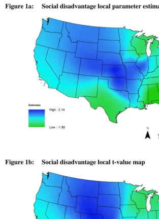
To better illustrate, we visualize the results of a GWR model where the county-level infant mortality rate is the outcome variable and social disadvantage (a composite variable) is the main predictor.5 Social disadvantage is a composite variable we have used in prior research (Yang, Teng, and Haran 2009; Chen et al. 2012). The Monte Carlo test results indicated that the association between social disadvantage and infant mortality is nonstationary across place. A rudimentary, but unsatisfactory strategy is to present two maps, one map showing the local parameter estimates for social disadvantage and the other map showing the local t-values for the same variable (see Figure 1a & 1b).
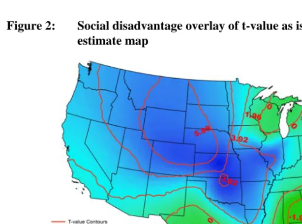
A more sophisticated approach is to overlay specific t-values (e.g., +/- 1.96) as isolines (or contour lines) on top of the parameter estimate surface (see Figure 2).6 The isolines can be defined for any set of data values (e.g., values that correspond to levels of statistical significance).7 The isoline method allows the map reader to read both the approximate parameter estimate and the t-value for any location on the map. In our example the isolines are relatively easy to interpret, but if the range of local t-values is wide, it may be difficult to read exact values, specifically when the isolines follow complex paths or are spaced relatively close together.
Another issue, common to all cartographic design, is the placement of text labels attached to the contour lines. In current GIS software these decisions can be automated based on optimum text-placement criteria, but this does not guarantee that the placement of text will not obscure salient areas of the map. The isoline approach places more burden on the map reader to recognize and then potentially eliminate from further consideration those parts of the map where the local t-value is not significant. That is, this map form does not place visual emphasis on the parts of the surface where local parameter estimates are significant. In our own work we have experimented with the isoline overlay approach, but in many of our applications we also wanted to show the basic outline of geographic areas (e.g., states or counties in US-based applications). When faced with such decisions regarding our own map design, the addition of isolines more often than not contributed to potential chartjunk (Tufte 1983) and possibly more confusion for the map reader. We required a more elegant mapping design for our GWR applications.
5 This simple model includes other controls (e.g., race/ethnic composition).
6 We note that Byrne, Charlton, and Fotheringham (2009) use an adjustment to take advantage of the
dependency between local GWR models based on a Bonferroni style adjustment for multiple hypotheses testing.
7
Figure 1a: Social disadvantage local parameter estimate map
Figure 2: Social disadvantage overlay of t-value as isolines on parameter estimate map
Mennis (2006) reminds GWR users that bivariate choropleth mapping is a viable approach for mapping the GWR parameter estimate and the local t-values simultaneously. Bivariate choropleth mapping was first introduced by Olson (1981); see also Eyton (1984) and Dunn (1989). Further Mennis combines a bivariate choropleth mapping with masking approaches that effectively limit the presentation of results to only those areas of the study area (the map) where t-values are significant. We adapt the approach of Mennis (2006).8
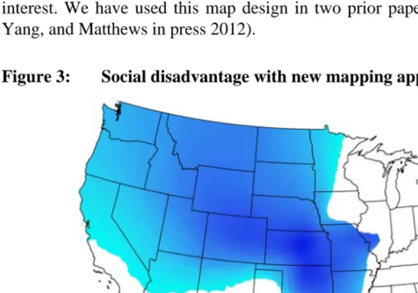
Briefly, in ArcGIS 10 (Esri 2011) we create the surface of estimated coefficients and the local t-values for a selected parameter, social disadvantage. Within ArcGIS 10 it is trivial to set up a mask in one data layer (i.e., the local t-values) and to order this to be visually above or on top of another data layer (i.e., the local parameter estimate). The t-value data layer is set up so that data values lying between -1.96 and +1.96 are masked out (showing white on Figure 3) while data values smaller than -1.96 or greater than +1.96 are set to 100% transparency. Transparency means that the data stored in
8 Our approach is based on the integrated use of GWR 3.0/4.0 and ArcGIS 10. Please contact the authors for a
another data layer below will be seen unobstructed. Whereas Mennis uses a data classification scheme based on standard-deviation and N-class methods (based on optimal methods for maximizing within-class homogeneity) we use a continuous bivariate color scheme for the parameter estimate surface. In Figure 3 the significant positive parameter estimates are represented by shades of blue, while the significant negative parameter estimates are shades of green. This map design facilitates map interpretation and immediately allows the map reader to identify locations of potential interest. We have used this map design in two prior papers (Chen et al. 2012; Shoff, Yang, and Matthews in press 2012).
Figure 3: Social disadvantage with new mapping approach
4. Discussion
health studies in light of the locality of health outcomes (Young and Gotway 2010). Moreover, it is argued that GWR can potentially make significant contributions to health research, such as allowing researchers to better understand the etiology and spatial processes, offering informative results beyond global models to facilitate place-specific health policy formation, and enabling scholars to explore questions that cannot be answered with traditional (global) analytical models. As we reported above, GWR is a useful exploratory technique in all demographic-related disciplines where spatial data are used, and in applications where spatial nonstationarity is suspected (and should be checked for).
Like other analytic methods, GWR has limitations, including issues associated with multicollinearity, kernel bandwidth selection, and multiple hypothesis testing (Wheeler and Tiefelsdorf 2005; Wheeler 2007, 2009; Cho et al. 2009; Jiang, Yao, and Wheeler 2010; Wheeler and Páez 2010). Some of these issues have been addressed (Wheeler 2007, 2009). GWR is generally regarded as a useful tool for exploring spatial nonstationarity and interpolation (Páez, Long, and Farber 2008; Wheeler and Páez 2010) but further testing is required (Páez, Farber, and Wheeler 2011).
In this brief paper we reviewed some standard but ultimately poor approaches to visualizing local parameter estimates. We offer a fairly simple map format based on the inherent strengths of a GIS and sound cartographic design that allows for two variables, specifically both local statistics – the parameter estimate and the t-value – to be mapped together, by laying one layer file above another layer. Using masking and transparency techniques on the local t-value layer we allow only the significant parameter estimate values to be visualized. This mapping template allows the map reader to focus on the primary areas of interest in the map. This approach represents a significant improvement over mapping all local parameter estimates irrespective of whether or not they are significant.9
5. Acknowledgements
This work was partially supported by internal funds from the Social Science Research Institute at Penn State. Additional support has been provided by the Geographic Information Analysis Core at Penn State's Population Research Institute, which receives core funding from the Eunice Kennedy Shriver National Institutes of Child Health and Human Development (R24-HD41025). We thank Nyesha Black, Aggie Noah, and Carla Shoff for their comments and suggestions regarding our manuscript. All errors remain our own.
9
References
Akaike, H. (1974). A new look at the statistical model identification. IEEE Transactions on Automatic Control 19(6): 716-723. doi:10.1109/ TAC.1974.1100705.
Ali, K., Partridge M.D., and Olfert M.R. (2007). Can geographically weighted regressions improve regional analysis and policy making? International Regional Science Review 30(3): 300-331. doi:10.1177/0160017607301609.
Benson, T., Chamberlin, J., and Rhinehart, I. (2005). An investigation of the spatial determinants of the local prevalence of poverty in rural Malawi. Washington DC: International Food Policy Research Institute.
Brewer, C.A. (1994). Color use guidelines for mapping and visualization. In: MacEachren, A. and Taylor, D.R.F. (eds.). Visualization in modern cartography.
New York: Elsevier: 123-147.
Brewer, C.A. (1996). Guidelines for selecting colors for diverging schemes on maps.
The Cartographic Journal 33(2): 79-86. doi:10.1179/000870496787757221.
Brunsdon, C., Fotheringham, A.S., and Charlton, M. (1998a). Spatial nonstationarity and autoregressive models. Environment and Planning A 30(6): 957-973. doi:10.1068/a300957.
Brunsdon, C., Fotheringham, A.S., and Charlton, M. (1998b). Geographically weighted regression: Modelling spatial non-stationarity. Journal of the Royal Statistical Society. Series D (The Statistician) 47(3): 431-443. doi:10.1111/1467-9884.00145.
Brunsdon, C., Fotheringham, A.S., and Charlton, M.E. (1996). Geographically weighted regression: A method for exploring spatial nonstationarity.
Geographical Analysis 28(4), 281-298. doi:10.1111/j.1538-4632.1996.tb00936.x.
Byrne, G., Charlton, M., and Fotheringham, S. (2009). Multiple dependent hypothesis tests in geographically weighted regression. In: Lees, B.G. and Laffan, S.W. (eds.). 10th International Conference on GeoComputation, UNSW, Sydney, November-December. http://www.biodiverse.unsw.edu.au/geocomputation/ proceedings/PDF/Byrne_et_al.pdf (February 1, 2012).
Chen, V.Y.-J., Deng, W.-S., Yang, T.-C., and Matthews, S.A. (2012). A geographically weighted quantile regression approach for spatial data analysis: An application to county-level U.S. mortality data. Geographical Analysis 44(2): 134-150. doi:10.1111/j.1538-4632.2012.00841.x.
Chen, V.Y.-J., Wu, P.-C., Yang, T.-C., and Su, H.-J. (2010). Examining non-stationary effects of social determinants on cardiovascular mortality after cold surges in Taiwan. Science of the Total Environment 408(9): 2042–2049. doi:10.1016/j.scitotenv.2009.11.044.
Chen, V.Y.-J. and Yang, T.-C. (2011) SAS macro programs for geographically weighted generalized linear modeling with spatial point data: Applications to health research. Computer Methods and Programs in Biomedicine. doi:10.1016/j.cmpb.2011.10.006.
Cho, S., Lambert, D.M., Kim, S.G., and Jung, S. (2009). Extreme coefficients in geographically weighted regression and their effects on mapping. GIScience and Remote Sensing 46(3): 273–288.doi:10.2747/1548-1603.46.3.273.
Cleveland, W.S. (1979). Robust locally weighted regression and smoothing scatterplots.
Journal of the American Statistical Association 74(368): 829–836. doi:10.2307/2286407.
Cressie, N.A.C. (1993). Statistics for spatial data. New York, NY: John Willey & Sons.
Dunn, R. (1989). A dynamic approach to two-variable color mapping. The American Statistician 43(4): 245-252. doi:10.2307/2685372.
Esri (2011). ArcGIS Desktop: Release 10. Redlands, CA: Environmental Systems Research Institute.
Eyton, J.R. (1984). Complementary-color, two-variable maps. Annals of the Association of American Geographers 74(3): 477-490. doi:10.1111/j.1467-8306.1984.tb01469.x.
Foody, G.M. (2003). Geographical weighting as a further refinement to regression modelling: An example focused on the NDVI-rainfall relationship. Remote Sensing of the Environment 88(3): 283-293. doi:10.1016/j.rse.2003.08.004.
Fotheringham, A.S., Brunsdon, C., and Charlton, M.E. (1997). Two techniques for exploring non-stationarity in geographical data. Geographical Systems 4: 59-82.
Fotheringham, A.S., Charlton, M.E., and Brunsdon, C. (1998). Geographically weighted regression: a natural evolution of the expansion method for spatial data analysis. Environment and Planning A 30(11): 1905-1927.doi:10.1068/a301905.
Goodchild, M.F. and Janelle, D.G. (2004). Spatially integrated social science. New York, NY: Oxford University Press.
Goovaerts, P. (2005). Analysis and detection of health disparities using geostatistics and a space-time information system: The case of prostate cancer mortality in the United States, 1970-1994. Proceedings of GIS Planet 2005. (May 30-June 2, 2005, Estoril, Portugal).
Gregory, I.N. and Ell, P.S. (2005). Analyzing spatiotemporal change by use of National Historical Geographical Information Systems: Population change during and after the Great Irish Famine. Historical Methods 38(4): 149-167. doi:10.3200/HMTS.38.4.149-167.
Hope, A.C.A. (1968). A simplified Monte Carlo significance test procedure. Journal of the Royal Statistical Society: Series B (Methodological) 30(3): 582-598
Huang, Y. and Leung, Y. (2002). Analyzing regional industrialization in Jiangsu province using geographically weighted regression. Journal of Geographical
Systems 4(2): 233–249doi:10.1007/s101090200081.
Jiang, B., Yao, X., and Wheeler, D.C. (2010). Visualizing and diagnosing coefficients from geographically weighted regression models. In: Sui, D.Z., Tietze, W., Claval, P., Gradus, Y., Park, S.O., and Wusten, H. (eds.). Geospatial analysis and modelling of urban structure and dynamics. Netherlands: Springer: 415-436. doi:10.1007/978-90-481-8572-6.
Jones, J.P.III. and Hanham, R.Q. (1995). Contingency, realism and the expansion method. Geographical Analysis 27(3): 185-207 doi:10.1111/j.1538-4632.1995.tb00905.x.
Jordan, L.M. (2006). Religion and demography in the United States: A geographical analysis. [Ph.D. Thesis]. Boulder, Colorado: University of Colorado at Boulder, Department of Geography.
Lloyd, C. (2011). Local models for spatial analysis(Second Edition). Boca Raton, FL: CRC Press.
Mennis, J.L. (2006). Mapping the results of geographically weighted regression. The Cartographic Journal 43(2): 171-179. doi:10.1179/000870406X114658.
Mennis, J.L. and Jordan, L.M. (2005). The distribution of environmental equity: exploring spatial nonstationarity in multivariate models of air toxic releases.
Annals of the Association of American Geographers 95(2): 249-268. doi:10.1111/j.1467-8306.2005.00459.x.
Nakaya, T., Fotheringham, A.S., Brunsdon, C., and Charlton, M. (2005). Geographically weighted Poisson regression for disease association mapping.
Statistics in Medicine 24(17): 2695-2717. doi:10.1002/sim.2129.
National Center for Geocomputation (2009). Maynooth, Ireland: National University of Ireland. http://ncg.nuim.ie/ncg/GWR/software.htm (Febuary 1, 2012).
Olson, J.M. (1981). Spectrally encoded two-variable maps. Annals of the Association of American Geographers 71(2): 259-276. doi:10.1111/j.1467-8306.1981.tb01352.x.
Páez, A., Farber, S., and Wheeler, D.C. (2011). A simulation-based study of geographically weighted regression as a method for investigating spatially varying relationships. Environment and Planning A 43(12): 2992-3010. doi:10.1177/0042098008091491.
Páez, A., Long, F., and Farber, S. (2008). Moving window approaches for hedonic price estimation: An empirical comparison of modelling techniques. Urban Studies
45(8): 1565-1581.doi:10.1177/0042098008091491.
Partridge, M.D. and Rickman, D.S. (2005). Persistent pockets of extreme American poverty: People or place based? Columbia, MO: Rural Poverty Research Center (RPRC). (Working Paper 05-02, Jaunary 2005).
R Development Core Team (2011). R: A language and environment for statistical computing [electronic resource]. Vienna, Austria: R Foundation for Statistical Computing. http://www.R-project.org (February 1, 2012).
Salas, C., Ene, L., Gregoire, T.G.E., Næsset, E., and Gobakken, T. (2010) Modelling tree diameter from airborne laser scanning derived variables: A comparison of spatial statistical models. Remote Sensing of Environment 114(6): 1277–1285. doi:10.1016/j.rse.2010.01.020.
Shoff, C., Yang, T.-C., and Matthews, S.A. (in press 2012). What has geography got to do with it? Using GWR to explore place-specific associations with prenatal care utilization. GeoJournal.doi:10.1007/s10708-010-9405-3.
Tufte, E. (1983). The visual display of quantitative information. Cheshire, CT: Graphics Press.
Wheeler, D.C. (2007). Diagnostic tools and a remedial method for collinearity in geographically weighted regression. Environment and Planning A 39(10): 2464-2481.doi:10.1068/a38325.
Wheeler, D.C. (2009). Simultaneous coefficient penalization and model selection in geographically weighted regression: The geographically weighted lasso.
Environment and Planning A 41(3): 722-742.doi:10.1068/a40256.
Wheeler, D.C. and Páez, A. (2010). Geographically weighted regression. In: Fischer, M.M. and Getis, A. (eds.). Handbook of applied spatial analysis: Software tools, methods and applications. Berlin and Heidelberg: Springer: 461-486. doi:10.1007/978-3-642-03647-7_22.
Wheeler, D.C. and Tiefelsdorf, M. (2005). Multicollinearity and correlation among local regression coefficients in geographically weighted regression. Journal of Geographical Systems 7(2): 161-187. doi:10.1007/s10109-005-0155-6.
Yang, T.-C., Teng, H.W., and Haran, M. (2009). The impacts of social capital on infant mortality in the U.S.: A spatial investigation. Applied Spatial Analysis and Policy 2(3): 211–227. doi:10.1007/s12061-009-9025-9.
Yang, T.-C., Wu, P.-C., Chen V.Y.-J., and Su H.-J. (2009). Cold surge: A sudden and spatially varying threat to health? Science of the Total Environment 407(10): 3421-3424.doi:10.1016/j.scitotenv.2008.12.044.
Young, L.J. and Gotway C.A. (2010). Using geostatistical methods in the analysis of public health data: The final frontier? geoENV VII - Geostatistics for Environmental Applications 16: 89-98. doi:10.1007/978-90-481-2322-3_8.
Yu, D.-L. (2006). Spatially varying development mechanisms in the Greater Beijing area: A geographically weighted regression investigation. Annals of Regional Science 40(1): 173-190.doi:10.1007/s00168-005-0038-2.
Zhao, F. and Park, N. (2004). Using geographically weighted regression models to estimate annual average daily traffic. In: Transportation Research Record1879.