Max Planck Institute for Demographic Research Konrad-Zuse Str. 1, D-18057 Rostock·GERMANY www.demographic-research.org
DEMOGRAPHIC RESEARCH
VOLUME 23, ARTICLE 27, PAGES 749-770
PUBLISHED 22 OCTOBER 2010
http://www.demographic-research.org/Volumes/Vol23/27/ DOI: 10.4054/DemRes.2010.23.27
Descriptive Findings
Age-adjusted disability rates and regional
effects in Russia
Aleksandr A. Andreev
Charles M. Becker
c
°2010 Aleksandr A. Andreev & Charles M. Becker.
2 The Russian disability system 751
3 Methodology 753
4 Results 757
5 Conclusion 768
Age-adjusted disability rates and regional effects in Russia
Aleksandr A. Andreev1
Charles M. Becker2
Abstract
We provide three measures of age-standardized disability rates for each Russian region and show that most, though not all, of the regional patterns in disability prevalence dis-appear with standardization. Disability prevalence remains unusually high for women in St Petersburg and Belgorod but the “remote but healthy” pattern is nearly gone. We conclude that differences in age structure largely account for the differences in disability prevalence across regions of Russia.
1Graduate Student, Department of Economics, University of North Carolina at Chapel Hill. The financial
support of the NSF Graduate Research Fellowship Program is gratefully acknowledged. Views expressed herein are solely those of the authors and do not reflect official policy of the National Science Foundation. E-mail: [email protected].
2Research Professor of Economics, Duke University. E-mail: [email protected]. The authors would like
1. Introduction
The prevalence of disability in transition nations is high, reflecting a combination of high prevalence of chronic disease, poor work-place safety practices, and relatively generous social safety net provisions (Andreev, 2008; Seitenova and Becker, 2008; Becker and Urzhumova, 1998). This high prevalence has attracted considerable discussion, and the presence of detailed data has made it possible to explore the characteristics of those receiv-ing disability payments in far more detail than is practical for most other middle-income countries. One of the superficially surprising characteristics concerns regional patterns of disability. Previous research has found that disability prevalence is lowest in Russia’s Far East and far north while highest in St Petersburg, Moscow, and the Central federal district. This is a counterintuitive finding, since the high prevalence regions are more prosperous and have better health care and social services. Based on anecdotal evidence, the discrep-ancies in disability prevalence across regions have been attributed to differences in the generosity of benefits, ease of access to the disability screening process or the prevalence of corruption or fraud. However, by incorporating the age structure of Russian regions, we conclude that almost all of the differences in disability prevalence can be attributed to differences in age structure, and that non-medical explanations are likely to be fairly unimportant.
Due to recent migration out of the Russian north and Far East, the population distri-bution in these regions is undoubtedly a product of self-selection on the basis of health and employment opportunity, which heavily correlate with age. Crude comparisons of disability prevalence rates across the regions of Russia may therefore be biased. A more appropriate method of comparison of disability rates would adjust for age. Such age-adjusted rates are already used in a number of applications, including mortality rates, incidence of cancer, and the like. This paper estimates age-adjusted disability rates on the basis of survey data of Russian households. In addition, the paper explores two other methods of capturing regional effects on disability prevalence using regression analysis.
With standardization, the “remote but healthy” advantage that appears to characterize Siberia, the Far East, and the northernmost regions almost disappears. A few significant gender differences in disability prevalence in some regions do remain. Even after stan-dardization, for example, disability rates for women in St Petersburg and Belgorod Oblast remain unusually high.
2. The Russian disability system
Disability in Russia is governed by the 24 November 1995 Federal law “On the Social Protection of Disabled Individuals in the Russian Federation.” The law defines as dis-abled an individual “who has a health impairment with a continued disruption of bodily functions caused by illness, the results of trauma, or [anatomical] defects, leading to lim-ited capacity for life and requiring social protection” (Russian Federation, 1995).
Russia has a complex federal system in which disability policy is set at the national level and administered by the regions.3 To obtain disabled status, an individual must
undergo a medical evaluation at the local office of the Bureau of Medical and Social Evaluation (BMSE). The evaluating committee votes on the applicant’s disabled status and assigns one of three disability groups, with Group I being most severe.4
Individuals with an assigned disability group who have an employment history are el-igible for “labor disability pensions” administered by the Russian Pension Fund, the same entity that provides pensions for the retired. Rules governing the type and amount of labor disability pension are governed by the 17 December 2001 Federal law “Concerning Labor Pensions.” In practice, all Group I, most Group II, and some of the Group III individuals with employment history are eligible. Those individuals who do not qualify for a labor disability pension may receive the smaller means-tested “social pension”, which is not dependent on employment history.
Very little is known about the likelihood of recovery from disability or the charac-teristics of the Russian disabled population or, for that matter, the disabled populations of middle-income countries in general. Notable exceptions include Mont (2007), Braith-waite and Mont (2008), Mete, BraithBraith-waite, and Schneider (2008), Scott and Mete (2008), and Hoopengardner (2001). There is also detailed presentation of disability patterns in Russia in Baskakov et al. (2001), Becker and Merkuryeva (2009), Schultz (2008), Mos-gorzdrav (2005), FBEA (1999), and FBEA (1998).
There has also been little study of the accuracy of the screening system or attempting to enumerate cases of benefits abuse, corruption or fraud. Using data from the RLMS, Merkuryeva (2007) examines the targeting accuracy of the Russian disability system and concludes that discrepancies in the system amount to roughly 13%. However, we should note that the health questions in the RLMS dataset do not completely capture the criteria used by the BMSE in evaluation, so this figure should be treated with some caution. That
3We use the term “regions” to refer to the administrative subdivisions (“Federal subjects”) of the Russian
Federation. These consist of 21 republics, 46 oblasti, 9 kraii, 1 autonomous oblast, 4 autonomous okrugi and 2 federal cities.
4In a recent reform, Groups I, II, and III were renamed as Categories 3, 2, and 1, respectively. We use the old
said, Merkuryeva (2007) also finds that discrepancies between health and disabled status increase with age; this provides one more reason to standardize disability rates by age.
Our study uses data from the Russian National Survey of Household Welfare and Participation in Social Programs, known by its Russian acronym as NOBUS. The NOBUS was conducted in 2003 by the Russian Federal Statistical Survey and the World Bank and is “a cross section survey of the Russian households, which was specially designed to measure the efficiency of the national social assistance programs by means of estimating the impact of social benefits and privileges on household welfare” (World Bank, 2003).
The NOBUS has a multi-stage stratified survey design, using sequential random se-lection. The population is divided into homogeneous strata based on the type of settle-ment. Within each stratum, primary sampling units (PSUs) were randomly selected. The PSUs are either settlements or, within large settlements, polling districts. Finally, within each PSU, households were selected at random. Within each household, a questionnaire was administered to each individual (the individual questionnaire) and to the head of household (the household questionnaire). Given such a survey design, observations in the NOBUS are not independent; thus, we use the appropriate econometric techniques for working with survey data, and reweigh observations to account for nonresponse, using the weights provided in the data.
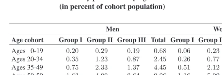
Table 1: Disability prevalence by age and sex cohort (in percent of cohort population)
Men Women
Age cohort Group I Group II Group III Total Group I Group II Group III Total
Ages 0-19 0.20 0.29 0.19 0.68 0.06 0.23 0.09 0.38 Ages 20-34 0.35 1.23 0.87 2.45 0.26 0.77 0.64 1.67 Ages 35-49 0.75 2.33 1.37 4.45 0.51 2.12 1.19 3.82 Ages 50-59 1.63 4.99 2.64 9.26 1.16 5.02 1.71 7.89 Ages 60-69 2.00 10.43 1.95 14.38 1.51 9.53 1.29 12.33 Ages 70 and up 2.46 18.87 2.28 23.61 1.98 16.35 1.44 19.76 Total 0.88 3.94 1.25 6.08 0.77 4.72 0.98 6.47
3. Methodology
In standard population counts, an age-adjusted rate may be computed as follows: Letδi be an indicator variable equal to one if theithindividual is disabled, and zero otherwise. Divide the population intoCage and sex cohorts. Then the age-specific disability rate for a given cohort is given by
ASDRc= 1
nc nc
X
i=1
δi (1)
wherencis the number of individuals in thecthcohort.
The age-adjusted disability rate is simply a weighted average of the ASDRs for all cohorts using a standard population to determine weights. Letpcbe the number of indi-viduals in thecthage cohort in the standard population. The total standard population is then
p=X
c
pc (2)
and the weight of thecthcohort is
wc =pc
We next compute the age-adjusted disability rate ADR as
ADR = X
c
wc∗ASDRc (4)
= 1
N
N
X
i=1
δiwi (5)
whereNis the total number of individuals in the population.
The above equations allow us to generalize this computation for survey data. Since the NOBUS dataset has a multi-stage survey design, we must rewrite Equation 4 taking into account survey sampling characteristics. Let our survey design sample primary sampling units (PSUs) from specified strata. It is easy to see that Equation 4 is simply the weighted mean of the disability indicator variableδi. Taking into account the survey design and the individual’s probability weights, the formula becomes
ADR= H X h=1 Jh X j=1 nhj X i=1 X c
δhjiwhjiwc
H X h=1 Jh X j=1 nhj X i=1 whji (6)
where we haveHstrata,JhPSUs in thehthstratum, andnhjobservations in thejthPSU of thehthstratum. Again,δ
hjiis the disabled status dummy of theithindividual in the
jthPSU of thehthstratum;w
c is the standardization weight of thecthage cohort; and
whjiis the sample weight, which reflects the probability that the individual was included in the sample.
The variance of the age-adjusted disability rate can be computed using formulae for variances of means in a complex survey (Graubard and Korn, 1996). Let the total weight of thejth PSU in thehth stratum beW
hj =
Pnhj
i=1whji and letADRhj be the age-adjusted disability rate in thejthPSU of thehthstratum. Then the variance is
ˆ
σADR2 =
1
³PH
h=1
PJh
j=1Whj ´2
H
X
h=1 Jh
Jh−1 Jh
X
j=1 ·
Whj(ADRhj−ADR)
− 1
Jh Jh
X
k=1
(ADRhk−ADR)
¸2 . (7)
by itself. That is, the purpose of standardized rates is to provide an ordinal ranking rather than a cardinal interpretation. Thus, any affine transformation of a standardized rate is equally appropriate, and hence the precise choice of standard population is not important, provided that the distribution chosen does not lead to ordinal rankings different from other plausible distribution choices.
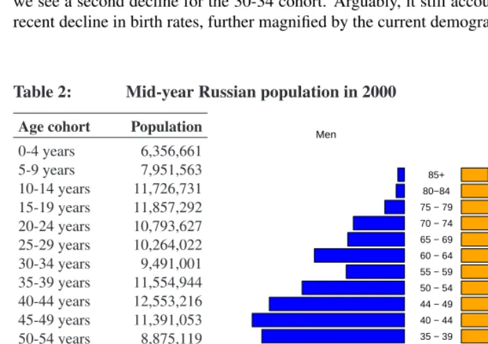
In practice, a convenient standard population is usually chosen in order to facilitate comparison with other studies. For the purposes of this study, we chose the 2000 mid-year Russian population as the standard. The standard population structure is presented in Table 2 and the accompanying age pyramid. The population structure reflects significant events in Russian history. The decline for those aged 55-59 is evidence of low birth rates during World War Two, which subsequently impacted birth rates in the late 60’s. Hence we see a second decline for the 30-34 cohort. Arguably, it still accounts for some of the recent decline in birth rates, further magnified by the current demographic situation.
Table 2: Mid-year Russian population in 2000
Age cohort Population
0-4 years 6,356,661 5-9 years 7,951,563 10-14 years 11,726,731 15-19 years 11,857,292 20-24 years 10,793,627 25-29 years 10,264,022 30-34 years 9,491,001 35-39 years 11,554,944 40-44 years 12,553,216 45-49 years 11,391,053 50-54 years 8,875,119 55-59 years 5,370,948 60-64 years 8,761,106 65-69 years 5,969,644 70-74 years 6,148,461 75-79 years 3,228,269 80-84 years 1,522,619 85 years and up 1,372,880
Total 145,189,156
Source:Goskomstat.
Men Women
(millions) 0 2 4 6 (millions)
0 2 4 6
0 − 4 5 − 9 10 − 14 15 − 19 20 − 24 24 − 29 30 − 34 35 − 39 40 − 44 44 − 49 50 − 54 55 − 59 60 − 64 65 − 69 70 − 74 75 − 79 80−84
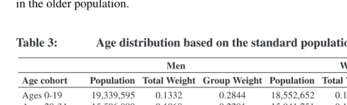
A few words are warranted about the choice of the number of cohorts. On the one hand, the larger the number of age cohorts, the better the analysis captures all the details of age-specific variation in disability rates. On the other hand, as the number of cohorts increases, the number of observations in each cohort decreases and the standard error of the age-adjusted disability rate estimate grows dramatically. Table 3 presents one possible grouping of age cohorts, which we will use for this study. Since the prevalence of disabil-ity increases unambiguously with age, this distribution imposes narrower age delineations in the older population.
Table 3: Age distribution based on the standard population
Men Women
Age cohort Population Total Weight Group Weight Population Total Weight Group Weight
Ages 0-19 19,339,595 0.1332 0.2844 18,552,652 0.1278 0.2403
Ages 20-34 15,506,899 0.1068 0.2281 15,041,751 0.1036 0.1948
Ages 35-49 17,323,234 0.1193 0.2548 18,175,979 0.1252 0.2354
Ages 50-59 6,468,365 0.0446 0.0951 7,777,702 0.0536 0.1008
Ages 60-69 5,910,016 0.0407 0.0869 8,820,734 0.0608 0.1143
Ages 70 and up 3,443,145 0.0237 0.0506 8,829,084 0.0608 0.1144
Total 67,991,254 0.4682 1.0000 77,197,902 0.5317 1.0000
We now present two alternative methods to capture regional effects on disability prevalence. In the first method, compute the crude disability rate for therthregion as
cdrr= 1
nr nr
X
i=1
δi. (8)
The next step is to regress across regions the crude disability rates obtained in Equation 8 on the number of individuals in each age cohort
cdrr=wr
X
c
βcnr,c+²r (9)
wherewr=nr/
P
rnris the weight of therthregion. The estimated coefficientsβˆcare the estimates of national age-specific disability rates and the residual²ˆrcaptures the fixed effect of therthregion not due to age structure. In theory, regions with high age-adjusted disability rates (computed as specified above) should have positive residuals and regions with low age-adjusted disability rates should have negative residuals.
in which the probability that theithindividual is disabled is
P[disabi= 1|I~i] = Φ
à β0+
X
r
βrIi,r+
X
c
βcIi,c+²i
!
(10)
whereIi,ris an indicator variable equal to one if theithindividual lives in therthregion and zero otherwise andIi,c is an indicator variable equal to one if theithindividual is in the cth age cohort and zero otherwise. Then the estimatedβˆ
c captures the national age-specific disability rate for cohortcand the estimatedβˆrcaptures the regional fixed effect.
In principle, other terms can be added to the regression in Equation 10. We add individual-specific variables that affect disability risk, including those variables found in standard prevalence analyses (see in particular Merkuryeva (2007); also Scott and Mete (2008), Hoopengardner (2001), and Schultz (2008)). The remaining regional effects are those that exist controlling for demographic structure as well as differences in compo-sition of individuals (who vary in terms of education, marital status and health-related measures), settlement properties (urban or rural), and regional prosperity (reflected in per capita household income).
By adding these terms, it is possible to compare unadjusted regional disability rates with age-standardized rates that do not correct for the environment, and then with stan-dardized rates that correct for individual and regional characteristics. We see that while most differences in prevalence across regions disappear with standardization, the remain-ing differences, with a few exceptions, disappear once we control for these individual characteristics.
4. Results
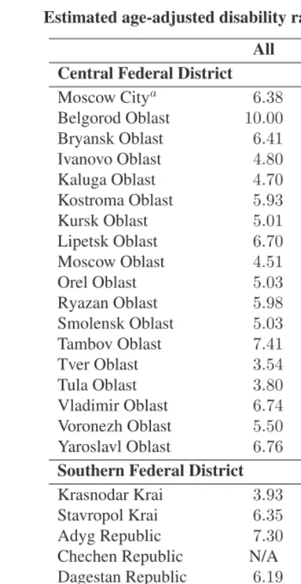
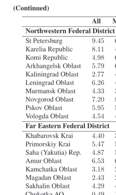
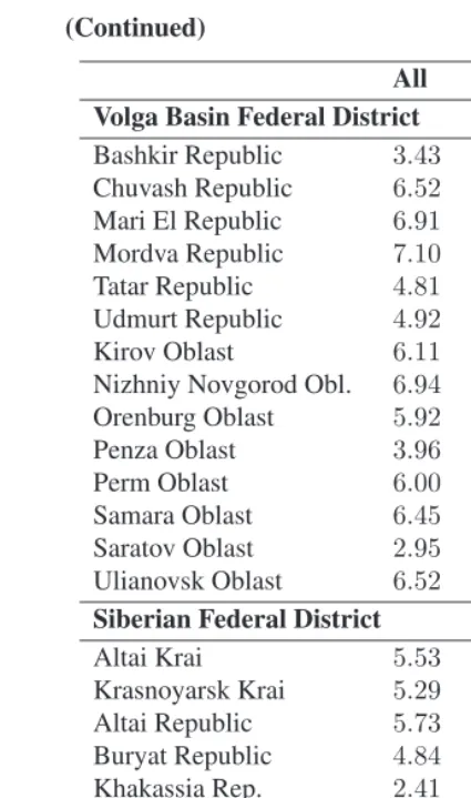
Table 4 presents the adjusted disability rates for 79 regions of the Russian Federation based on the first standardization approach (data for Chechnya are not available). The first column reports the sex- and adjusted rate and the next two columns report age-adjusted rates for men and women separately.5 Observe that the highest sex- and
age-adjusted disability rates are in Belgorod Oblast and the lowest are in Chukotka AO. Split-ting the sample along gender lines reveals a more complex trend: for women, the highest disability rates are in St Petersburg, Belgorod Oblast, Karelia Republic, and the Jewish AO; the lowest are in in Chukotka and Kaliningrad Oblast. For men, the highest ad-justed rates are in the Karachay-Cherkess Republic while the lowest are in Chukotka and Khakassia Republic.
5We also computed overall age-adjusted rates without adjusting for sex. These are almost identical to the
Table 4: Estimated age-adjusted disability rates in the regions of Russia All Men Women
Central Federal District
Moscow Citya 6.38 4.41 8.10
Belgorod Oblast 10.00 7.81 11.93
Bryansk Oblast 6.41 6.98 5.91
Ivanovo Oblast 4.80 5.89 3.83
Kaluga Oblast 4.70 7.64 2.10
Kostroma Oblast 5.93 5.35 6.45
Kursk Oblast 5.01 5.01 5.01
Lipetsk Oblast 6.70 7.23 6.22
Moscow Oblast 4.51 4.36 4.64
Orel Oblast 5.03 4.84 5.21
Ryazan Oblast 5.98 7.00 5.08
Smolensk Oblast 5.03 4.22 5.74
Tambov Oblast 7.41 7.75 7.11
Tver Oblast 3.54 4.55 2.65
Tula Oblast 3.80 3.25 4.28
Vladimir Oblast 6.74 7.40 6.16
Voronezh Oblast 5.50 5.51 5.49
Yaroslavl Oblast 6.76 6.77 6.75
Southern Federal District
Krasnodar Krai 3.93 3.86 3.99
Stavropol Krai 6.35 5.33 7.24
Adyg Republic 7.30 7.61 7.04
Chechen Republic N/A N/A N/A
Dagestan Republic 6.19 5.75 6.57
Ingush Republic 4.16 5.05 3.37
Kabardino-Balkar Rep. 4.58 4.63 4.52
Kalmyk Republic 5.04 5.35 4.76
Karachay-Cherkess Rep. 6.45 9.03 4.17
North Ossetin Rep. 5.22 6.49 4.10
Astrakhan Oblast 2.70 3.44 2.06
Rostov Oblast 6.45 5.49 7.30
Table 4: (Continued)
All Men Women Northwestern Federal District
St Petersburg 9.45 6.19 12.34
Karelia Republic 8.11 4.64 11.18
Komi Republic 4.98 6.29 3.82
Arkhangelsk Oblast 5.79 6.34 5.31 Kaliningrad Oblast 2.77 4.54 1.21 Leningrad Oblast 6.26 4.99 7.38 Murmansk Oblast 4.33 3.47 5.09 Novgorod Oblast 7.20 8.48 6.06
Pskov Oblast 5.95 5.83 6.06
Vologda Oblast 4.54 4.31 4.75
Far Eastern Federal District
Khabarovsk Krai 4.40 3.26 5.40 Primorskiy Krai 5.47 5.88 5.10 Saha (Yakutia) Rep. 4.87 5.38 4.43
Amur Oblast 6.53 6.01 7.00
Kamchatka Oblast 3.18 2.05 4.17
Magadan Oblast 2.43 2.80 2.10
Sakhalin Oblast 4.29 4.29 4.29
Chukotka AO 0.49 1.07 0.00
Jewish AO 6.99 2.46 10.98
Uralic Federal District
Chelyabinsk Oblast 3.82 3.98 4.05
Kurgan Oblast 3.84 4.56 3.22
Sverdlovsk Oblast 5.37 4.97 5.72
Table 4: (Continued)
All Men Women Volga Basin Federal District
Bashkir Republic 3.43 3.80 3.11
Chuvash Republic 6.52 6.15 6.85
Mari El Republic 6.91 7.24 6.62
Mordva Republic 7.10 8.19 6.15
Tatar Republic 4.81 5.39 4.29
Udmurt Republic 4.92 5.94 4.02
Kirov Oblast 6.11 6.31 5.94
Nizhniy Novgorod Obl. 6.94 6.15 7.64
Orenburg Oblast 5.92 4.35 7.31
Penza Oblast 3.96 4.51 3.48
Perm Oblast 6.00 5.39 6.53
Samara Oblast 6.45 6.69 6.23
Saratov Oblast 2.95 2.01 3.78
Ulianovsk Oblast 6.52 8.22 5.03
Siberian Federal District
Altai Krai 5.53 5.79 5.31
Krasnoyarsk Krai 5.29 5.59 5.03
Altai Republic 5.73 4.33 6.96
Buryat Republic 4.84 4.25 5.37
Khakassia Rep. 2.41 1.21 3.47
Tuva Republic 2.87 2.09 3.55
Chita Oblast 6.65 6.34 6.92
Irkutsk Oblast 5.50 5.12 5.83
Kemerovo Oblast 3.82 4.34 3.36
Nobosibirsk Obl. 4.18 4.67 3.75
Omsk Oblast 5.77 5.99 5.57
Tomsk Oblast 4.01 3.96 4.05
aThe regions are identified according to their 2003 names and boundaries. Since then, some regions have
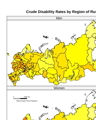
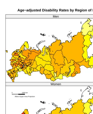
Figure 1 plots the overall adjusted disability rate against the overall crude disability rate. For ease of comparison, we have scaled both variables to zero mean and unity variance (recall that this transformation preserves the ordinal rankings). We observe that remote regions – those in the north, Siberia and Far East – tend to be above the 45-degree line (we have identified Karelia in the north, Altai on the Mongolian border and the Jewish AO in the Far East) – while more populous central regions tend to be below the 45-degree line (for example, St Petersburg, Moscow and its suburbs). This confirms that differences in age structure are at play. To help further visualize the effect of standardization, we plot crude and age-adjusted disability rates on a map of the Russian Federation in Figure 2. The maps reveal that with standardization some, though not all, of the counter-intuitive “remote but healthy” pattern is gone.
Figure 1: Overall age-adjusted vs. crude disability rates in regions of Russia
−4 −2 0 2 4
−4
−2
0
2
4
Crude Disability Rate
Adjusted Disability Rate
St. Petersburg
Moscow City
Moscow Obl Altai Republic
Karelia
Figure 2: Crude and age-adjusted disability rates
Crude Disability Rates by Region of Russia
Men
0 1000 km Albers Equal−Area Projection
GIS data Copyright 1998 Alexander Perepechko and Dmitry Sharkov.
Women
Figure 2: (Continued)
Age−adjusted Disability Rates by Region of Russia
Men
0 1000 km Albers Equal−Area Projection
GIS data Copyright 1998 Alexander Perepechko and Dmitry Sharkov.
Women
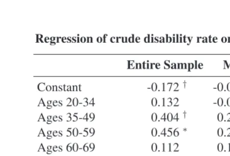
What is the quantitative impact of age structure on the regional crude disability rate? We can answer this question by looking at the regional effect regressions using group data, presented in Table 5. The coefficients confirm that disability prevalence increases with age. However, the coefficients for the cohort aged 60-69 are insignificant. Members of the group aged 60-69 at the time of data collection were born in 1934-1943. It is possible that the statistical insignificance of these coefficients captures effects of Soviet collectivization policies in the 1930’s and the Second World War era. This is a small birth cohort, and it is possible that premature mortality for many would have led to a survival bias.6
Table 5: Regression of crude disability rate on age cohorts over the regions Entire Sample Men Women
Constant -0.172† -0.0621 -0.300
Ages 20-34 0.132 -0.0022 0.352
Ages 35-49 0.404† 0.263∗ 0.543†
Ages 50-59 0.456∗ 0.245∗∗ 0.608∗
Ages 60-69 0.112 0.115 0.147
Ages 70 and above
0.413∗∗ 0.255∗∗ 0.593∗∗
Number of Obs. 79
R2 0.54 0.45 0.47
F on 5 and 73 df 10.56∗∗ 14.96∗∗ 8.17∗∗
Significance levels:†:10%,∗:5%,∗∗:1%
Second, the age coefficients for women are almost double those of their male counter-parts. Especially striking is the large coefficient on women aged 50-59; a one-tenth unit increase in the share of this cohort would account for an increase in the crude disabil-ity rate of six percentage points. We believe this is a consequence of the retirement age for women set at 55; upon retiring many individuals apply for disabled status in order to qualify for additional social benefits.
The regional effect residuals are plotted against the age-adjusted disability rates in Fig-ure 3. Again, both values have been standardized to have zero mean and unity variance. The high degree of collinearity between these measures confirms that the standardization
6This is not inconsistent with an effect, suggested below, of being a survivor of the Siege of Leningrad, since
procedure is robust. The only two exceptions are Chukotka AO and Tuva; the standard-ized rates and residuals differ considerably, probably because of the small number of observations in these two (most remote) regions.
Figure 3: Age-adjusted disability rates and regional effect residuals
−4 −2 0 2 4
−4 −2 0 2 4 Entire Sample
Adjusted Disability Rate
Regional Eff
ect
Chukotka Tuva
−4 −2 0 2 4
−4 −2 0 2 4 Men
Adjusted Disability Rate
Regional Eff
ect
Chukotka
Karachaevo−Cherkessia
Tuva
−4 −2 0 2 4
−4 −2 0 2 4 Women
Adjusted Disability Rate
Regional Eff
ect
Chukotka Tuva
−4 −2 0 2 4
−4
−2
0
2
4
Men vs. Women
Finally, Table 6 presents the probit regression results. Initially, we regress disabled status on region of residency and age cohort for both women and men. As expected from the age-adjustment computations, we observe statistically significant and positive coefficients for women in Belgorod Oblast and St Petersburg. We observe a negative and statistically significant coefficient for women in Astrakhan Oblast, which agrees with the low age-adjusted rate for that region. For men, we observe negative and statistically significant coefficients in Kamchatka and Khakassia. Both of these regions also have low age-adjusted rates. The coefficients on other regions are not significant once we control for age structure.
How much regional variation remains after controlling for age? To answer this ques-tion, we run a second set of regressions, adding the following variables: health improved, a categorical variable coded as 1 if the individual reported that his health improved in the last year, 0 if it stayed the same, or -1 if it got worse; indicator variables for the type of settlement in which the individual lives; indicator variables for the individual’s education and family status; and the logarithm of total per capita household consumption, a proxy for poverty.
We note that disabledwomenare more likely to live in cities, to be single, and to have only elementary or secondary education. Improved health is negatively associated with disability, though the causality and timing here are unclear. In particular, we know that the individual reported that her health got worse (or better) in the last year, but we do not know how long she has been officially disabled. Per capita consumption is positively associated with disability, a counter-intuitive finding. Finally, observe that when we do add these additional variables, the coefficients on the regions tend to become smaller or less significant. This indicates that the remaining variation between regions can be explained by these behavioral variables. However, high female disability in Belgorod and St Petersburg remains unexplained. In the case of St Petersburg, the high prevalence of disability may be attributed to a large cohort of survivors of the 1941-1944 Siege of Leningrad, many of whom legally qualify for special social benefits, including disabled status.
Disabledmenare also more likely to live in cities and to be single. However, education effects for men are different than for women; in particular, tertiary education is associated with a lower probability of becoming disabled. This indicates, perhaps, that much of male disability may be occupational. The poverty proxy is insignificant.
Table 6: Probit estimation results (dependent variable: disabled)
Women Men
Regiona
Astrakhan Oblast -0.469∗∗ -0.489∗ -0.307† -0.314† Belgorod Oblast 0.525∗∗ 0.517∗ 0.226 0.269 Kaliningrad Oblast -0.661∗ -0.610† -0.163 -0.083 Kamchatka Oblast -0.115 -0.124 -0.495∗∗ -0.518∗∗ Tver Oblast -0.362∗ -0.313† -0.123 0.086 Saint Petersburg 0.568∗∗ 0.464∗ 0.064 0.021 Khakassia -0.197 -0.266 -0.925∗ -0.932∗ Age Cohortsb
Ages 20-34 0.543∗∗ 0.704∗∗ 0.506∗∗ 0.711∗∗ Ages 35-49 0.898∗∗ 1.133∗∗ 0.769∗∗ 1.139∗∗ Ages 50-59 1.249∗∗ 1.425∗∗ 1.144∗∗ 1.510∗∗ Ages 60-69 1.510∗∗ 1.630∗∗ 1.415∗∗ 1.731∗∗ Ages 70+ 1.806∗∗ 1.873∗∗ 1.756∗∗ 1.995∗∗ Health Improved -0.260∗∗ -0.442∗∗ Residencyc
Large City 0.275∗∗ 0.177∗
City 0.208∗∗ 0.068
Town 0.193∗∗ 0.016
Educationd
Primary 0.105 -0.175†
Incomplete Secondary 0.217∗∗ -0.130
Secondary 0.234∗∗ -0.083
PTU or FZU 0.136 -0.206∗
Vocational 0.106 -0.188†
Tertiary -0.119 -0.425∗∗
Family Statuse
Married -0.369∗∗ -0.499∗∗
Cohabitating -0.405∗∗ -0.438∗∗
Widowed -0.253∗∗ -0.483∗∗
Divorced / separated -0.282∗∗ -0.215∗∗ log(HH Consumption per capita) 0.101∗ -0.027 Constant -2.723∗∗ -3.779∗∗ -2.415∗∗ -2.169∗∗ Number of Obs. 64,975 52,065 Percent disabled 6.47% 6.08%
Significance levels:†: 10%,∗: 5%,∗∗: 1%.
aTotal of 79 regions, reporting only statistically significant coefficients. Omitted dummy: Altai Krai.
5. Conclusion
We observe that with age-adjustment, much of the unusual pattern in disability prevalence rates in Russia disappears. Adjusted disability rates remain low for men in Kamchatka and Khakassia, the only remaining portion of the “remote but healthy” pattern. The disability rates for women remain unusually high in St Petersburg and Belgorod Oblast, despite standardization and control for additional individual characteristics. At least in the case of St Petersburg, it is possible that this can be attributed to residual effects of World War Two.
What we do not find is evidence that inhabitants of central regions are “softer” (in the sense of being more sensitive to chronic conditions) or more effective in petitioning for disability status. Of course, it is possible that those in central regions are actually healthier than those in remote areas, and that greater sensitivity and petitioning ability by the former group acts as equalizing force. All that we can say, with reasonable certainty, is that this force does not overcompensate.
References
Andreev, A.A. (2008). To work or not to work: Labor supply decisions of Russia’s disabled.Duke Journal of Economics20 (special undergraduate research symposium). http://econ.duke.edu/dje/2008 Symp/Andreev.pdf.
Baskakov, V.N., Andreeva, O.N., Baskakova, M.E., Kartashov, G.D., and Krylova, E.K. (2001). Insurance for work-place accidents: Actuarial bases. [Страхование от несчастных случаев на производстве: актуарные основы]. Moscow, Russia: Academia.
Becker, C.M. and Merkuryeva, I.S. (2009). Disability incidence and official health sta-tus transitions in Russia. [unpublished manuscript]. Durham, NC: Duke University Department of Economics.
Becker, C.M. and Urzhumova, D.S. (1998). Pension burdens and labor force partici-pation in Kazakstan. World Development 26(11): 2087–2103. doi:10.1016/S0305-750X(98)00107-7.
Braithwaite, J. and Mont, D. (2008). Disability and poverty: A survey of World Bank assessments and implications. Washington, DC: World Bank. (Social Protection dis-cussion paper #0805).
FBEA (1998). Disability increase in Russia: Causes, trends, forecasts. [Рост инвалидности в России: причины, тенденции, прогнозы. Информационно-аналитический бюллетень Фонда «Бюро экономического анализа» #4]. Moscow, Russia: FBEA. (Analytical bulletin of the Foundation “Bureau of Economic Analysis”).
FBEA (1999). Disabled in Russia: Causes and dynamics of disability, contradictions and prospects for social policy [Инвалиды в России: причины и динамика инвалидности, противоречия и перспективы социальной политики. Информационно-аналитический бюллетень Фонда «Бюро экономического анализа»]. Moscow, Russia: FBEA. (Analytical bulletin of the Foundation “Bureau of Economic Analysis”).
Graubard, B.I. and Korn, E.L. (1996). Survey influence for subpopulations. American Journal of Epidemiology144(1): 102–106.
Hoopengardner, T. (2001). Disability and work in Poland. Washington, DC: World Bank. (Social Protection discussion paper #0101).
University, Graduate School of Management. http://pdc.ceu.hu/archive/00003798/. Mete, C., Braithwaite, J., and Schneider, P.H. (2008). Introduction. In: Mete, C. (ed.)
Economic Implications of Chronic Illnesses and Disability in Eastern Europe and the Former Soviet Union. Washington, DC: World Bank: 3–32.
Mont, D. (2007). Measuring disability prevalence. Washington, DC: World Bank. (Social Protection discussion paper #0706).
Mosgorzdrav (2005). Report on the health conditions in the City of Moscow for 2005 [Доклад о состоянии здоровья населения Москвы в 2005 году]. [electronic resource]. Moscow, Russia: Moscow City Department of Health. http://www.mosgorzdrav.ru/mgz/KOMZDRAVsite.nsf/f4ff3ec30c9e9687c325710d 0062f9e2/195f4011d052d18ac32570e4003e7c16.
Russian Federation (1995). Federal Law N181-F3, Concerning the social protection of disabled individuals in the Russian Federation. [О социальной защите инвалидов в Российской Федерации].
Schultz, T.P. (2008). Health disabilities and labor productivity in Russia in 2004. In: Mete, C. (ed.)Economic Implications of Chronic Illnesses and Disability in Eastern Europe and the Former Soviet Union. Washington, DC: World Bank: 85–118.
Scott, K. and Mete, C. (2008). Measurement of disability and linkages with welfare, employment, and schooling. In: Mete, C. (ed.)Economic Implications of Chronic Illnesses and Disability in Eastern Europe and the Former Soviet Union. Washington, DC: World Bank: 35–66.
Seitenova, A. and Becker, C.M. (2008). Disability in Kazakhstan: An evaluation of offi-cial data. Washington, DC: World Bank. (Sooffi-cial Protection discussion paper #0802). World Bank (2003). Russian Federation - NOBUS. [electronic resource]. Washington,