Comparative Hydrodynamic Testing of Small Scale Models

(1)

University of New Orleans University of New Orleans

ScholarWorks@UNO

University of New Orleans Theses and

Dissertations Dissertations and Theses

12-19-2008

Comparative Hydrodynamic Testing of Small Scale Models

Jared Acosta

University of New Orleans

Follow this and additional works at: https://scholarworks.uno.edu/td

Recommended Citation Recommended Citation

Acosta, Jared, "Comparative Hydrodynamic Testing of Small Scale Models" (2008). University of New Orleans Theses and Dissertations. 864.

https://scholarworks.uno.edu/td/864

(2)

rights-Comparative Hydrodynamic Testing of Small Scale Models

A Thesis

Submitted to the Graduate Faculty of the University of New Orleans

in partial fulfillment of the requirements for the degree of

Master of Science in

Engineering

Naval Architecture & Marine Engineering

by

Jared Acosta

B.S. University of New Orleans, 2005

(3)

LIST OF TABLES

(5)

LIST OF FIGURES

Figure 1 – Hybrid Catamaran Air Cushion (HCAC) side hull ... 1

Figure 2 – Round bilge side hull ... 2

Figure 3 – Hard chine side hull ... 2

Figure 4 – CNC milling of the test models ... 5

Figure 5 – Completed test models ... 6

Figure 6 – Force balance CAD model ... 8

Figure 7 – Completed force balance ... 9

Figure 8 – Force diagram ... 10

Figure 9 – Free-body diagram ... 10

Figure 10 – Translation of forces ... 12

Figure 11 – Carriage interface ... 13

Figure 12 – Example time history... 16

Figure 13 – Zeroed force data ... 17

Figure 14 – Hull A drag force ... 18

Figure 15 – Hull B drag force ... 19

Figure 16 – Hull C drag force ... 20

Figure 17 – Hull A lift force ... 21

Figure 18 – Hull B lift force ... 21

Figure 19 – Hull C lift force ... 22

Figure 20 – Hull A pitch moment ... 22

Figure 21 – Hull B pitch moment ... 23

Figure 22 – Hull C pitch moment... 23

Figure 23 – 0 degree trim drag force comparison ... 24

Figure 24 – ½ degree trim drag force comparison ... 25

Figure 25 – 1 degree trim drag force comparison ... 26

Figure 26 – 0 degree trim lift force comparison... 27

Figure 27 – ½ degree trim lift force comparison... 27

Figure 28 – 1 degree trim lift force comparison... 28

Figure 29 – 0 degree trim pitch moment comparison ... 29

Figure 30 – ½ degree trim pitch moment comparison ... 29

Figure 31 – 1 degree trim pitch moment comparison ... 30

(6)

NOTATION

g Acceleration due to gravity (32.2 ft/s2)

L Length

LM Length at model scale

LS Length at full scale

λ Scale Factor (LS/ LM)

V Velocity

VM Velocity at model scale

VS Velocity at full scale

Fn Froude number

F Net force applied to the model

FX’ X-component of translated net force

FZ’ Z-component of translated net force

M’ Moment created by translated net force

RV1 Force measured by forward vertical load cell

RV2 Force measured by aft vertical load cell

RH Force measured by horizontal load cell

h Vertical distance between model deck and bottom pins

l Horizontal distance between vertical load cell pins

L Calculated lift force

D Calculated drag force

(7)

ABSTRACT

Early in the ship design process, naval architects must often evaluate and compare multiple hull forms for a specific set of requirements.

Analytical tools are useful for quick comparisons, but they usually specialize in a specific hull type and are therefore not adequate for comparing

dissimilar hull types. Scale model hydrodynamic testing is the traditional evaluation method, and is applicable to most hull forms. Scale model tests are usually performed on the largest model possible in order to achieve the most accurate performance predictions. However, such testing is very

resource intensive, and is therefore not a cost effective method of evaluating multiple hull forms. This thesis explores the testing of small scale models. It is hypothesized that although the data acquired by these tests will not be accurate enough for performance predictions, they will be accurate enough to rank the performance of the multiple hull forms being evaluated.

(8)

INTRODUCTION

The premise of this thesis is a research and development project funded by Textron Marine & Land Systems. In 2006, Textron Innovations, Inc. patented the Hybrid Catamaran Air Cushion Ship (HCAC), shown in Figure 1.

Figure 1 – Hybrid Catamaran Air Cushion (HCAC) side hull

The HCAC, designed by inventors Kenneth Maloney and Charles Whipple, is capable of efficient operation at low speed as a traditional

catamaran and at high speed as a surface effect ship (SES). The HCAC main propulsor was a hybrid surface piercing propeller designed by Dr. William Vorus. This propeller complemented the HCAC nicely in that it was capable of efficient operation in both a low speed, fully submerged mode and a high speed, partially submerged mode. Although this propeller offers the most efficient operation, it is not well suited for beaching operations where the propeller blades could become damaged as the ship ran aground.

Waterjet propulsion is more suited for operations where the ship is required to operate in very shallow water or run aground. The HCAC hull form, however, is not well suited for waterjet propulsion. Having been designed with a propeller in mind, the side hull transom of the HCAC is very narrow and not capable of mounting a waterjet. Textron Marine & Land Systems sought to design an alternative to the HCAC side hull that would be capable of housing a waterjet. The author designed two alternatives to the HCAC side hull.

(9)

retain the exceptional low speed efficiency of the HCAC side hull. The round bilge hull is shown in Figure 2.

Figure 2 – Round bilge side hull

The second side hull was a hard chine design with a flat inboard side, similar to traditional SES side hulls. A review of performance data from the HCAC and other SES craft indicated that the hard chine design, while

possibly suffering a drag penalty at low speed, would provide increased efficiency at high speed. The hard chine hull is shown in Figure 3.

Figure 3 – Hard chine side hull

(10)

Existing analytical methods, although quick and relatively inexpensive, would not be able to fairly compare the alternative hull forms. For the most part, analytical methods either specialize in round bilge displacement type hulls or hard chine planning type hulls, but not both. For a fair comparison, the same evaluation method had to be used on both hulls. Analytical

methods also require a specialized skill set to yield quality results.

Traditional experimental methods involve the hydrodynamic testing of scale models in a tow tank, and would be capable of evaluating both hull forms. These types of experiments are usually carried out with the largest model possible in order to produce data that can be used to make full scale performance predictions. Obtaining scalable data for a large vessel requires a tow tank of sufficient length and speed capabilities. Large tow tanks are hard to come by, especially in the United States. Testing abroad introduces export issues that can be cumbersome and time consuming. Also, the cost of building and testing multiple large scale models was well beyond the budget of this project.

It was theorized that the testing of small scale models would be sufficient for this project. Small scale models would be relatively quick and inexpensive to build, and could be tested in the tow tank facility at the nearby University of New Orleans. The model scale would probably be too small to produce scalable data, but the intention of the project was to

(11)

CHAPTER 1 – TEST MODELS

Test Model Design

The tow tank at the University of New Orleans measures 101.5 ft long by 15.09 ft wide by 7.87 ft deep. The unmanned towing carriage is capable of usable speeds up to 9 ft/s. It is this speed that will set the scale factor for the models.

The models were Froude scaled, meaning that the Froude number for the model was equal to the Froude number for the ship. Froude number is given in Equation 1.

gL

V

F

_n

2

=

₍₁₎

Substituting the scale factor λ for LS/LM and solving for model speed VM

gives Equation 2.

λ

S M

V

=

₍₂₎

The maximum full scale speed tested was 40 knots. A scale factor of 1:60 resulted in a maximum model scale speed of 8.7 ft/s, which was within the capabilities of the tow tank carriage. This is the model scale that was chosen for the tests.

To further simplify testing, it was decided to test only a single side hull. The wet deck that connects the port and starboard side hulls, as well as the air cushion, would be omitted from the models. The wet deck only becomes wetted in rough sea conditions. Since these models would only be tested in calm water, the wet deck would have no influence on the

(12)

Test Model Fabrication

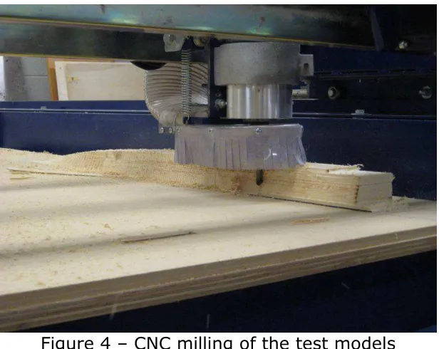
The test models were fabricated by George Morrissey in the UNO model fabrication laboratory using a three-axis CNC mill. The models were cut from poplar, a common wood used in ship model construction. The HCAC side hull and the round bilge side hull were milled in two separate pieces. The models were split at the side hull centerline, and the inboard and outboard halves were milled separately. After milling was complete, the two halves were glued together to form the complete side hull. The hard chine side hull, having a flat inboard side, was milled as a single piece. Figure 4 shows the CNC mill at work on one of the models.

Figure 4 – CNC milling of the test models

(13)

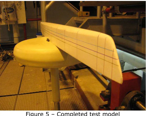
Figure 5 – Completed test model

(14)

CHAPTER 2 – FORCE BALANCE

Test Method

Traditional tow tank testing fixes the model motions in sway, yaw and roll. Although methods vary depending on the type of model being tested and the capabilities of the test facility, the most common method of testing focuses on the vertical plane motions. Surge is provided by the carriage, and the hydrodynamic drag is measured by force sensors. The model is usually free to heave and pitch, and the magnitude and direction of these motions are usually recorded. When the test run starts, the carriage pushes the model forward though the water. The heave and pitch of the model change as the model moves down the tank until the model comes into equilibrium. At the end of the run, the carriage decelerates and comes to a stop at the end of the tank. To obtain accurate data, drag force along with heave and pitch displacements must only be averaged in the equilibrium portion of the test run.

The test method presented here differs from traditional tow tank

testing in that forces are measured instead of motions. The model is fixed in all degrees of freedom, and lift force and pitch moment are measured

instead of heave displacements and angular pitch displacement. This test method has several advantages. First, since the attitude of the model does not change during the run, the model does not have to transition into an equilibrium position. There is still a transitional region near the beginning of the run where the model is developing its wave patterns, but this is largely accomplished during the period when the carriage is accelerating. This results in a larger useful time window for data averaging. Second, since the model is fixed in all degrees of freedom, it does not have to be ballasted to achieve the desired test conditions. The model draft and trim can be

changed easily without having to add or redistribute weight, saving time and effort during testing.

Force Balance Design & Construction

A force balance had to be designed that could measure drag force, lift force and pitch moment while fixing the model in sway, yaw and roll.

Although multi-axis load cells exist which measure all three forces and moments, these are expensive and only readily available in high load

(15)

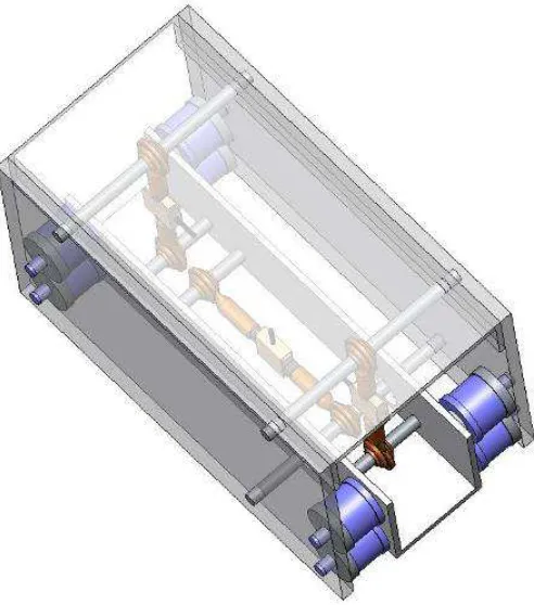
model in any axis other than the one it was measuring. The author developed the design shown in Figure 6, which utilizes three fairly inexpensive single-axis load cells.

Figure 6 – Force balance CAD model

(16)

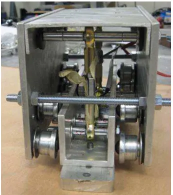
specified dimensions. The channel components were limited to catalogue availability, but the 3-D CAD model aided in the selection of components that would ensure fitment. Cut sheets with hole locations were printed for the aluminum plate and channel to ensure that the pin holes lined up properly. The constructed force balance is shown in Figure 7.

Figure 7 – Completed force balance

The force balance would undergo several slight mechanical

modifications before the design was successful. Threaded rod was added between the aluminum plates that make up the sides of the upper U-channel in order to control the squeezing load imparted on the lower U-channel. The fairly large ball transfers were also replaced with miniature ball transfer that could be independently adjusted to provide just the right amount of control to the lower U-channel.

Resolution of Forces

(17)

Figure 8 – Force diagram

The combination of the hydrodynamic and hydrostatic forces applied to the model result in the net force vector F. The direction of this vector and the location where it is applied to the model are unknown. However, the vector F can be translated into two forces and one moment applied at any point defined on the model. The forces and moment are FX’, FZ’ and M’,

respectively. The point O that these forces are applied at corresponds with the deck of the model directly in between the two vertical load cells.

A free-body diagram can be constructed by cutting the force balance through the load cell links. The free-body diagram is shown in Figure 9.

Figure 9 – Free-body diagram

(18)

0 =

∑

F

X (3)

0 '

₋

₌

H X

R

F

(4) H X

R

F

'

=

₍₅₎

The sum of forces in the y-direction is shown in Equations 6-8.

0 =

∑

F

Z (6)

0 '

₊

₁

₊

₂

₌

V V

Z

R

F

(7) 2 1

'

V V

Z

R

F

=

−

(8)

The sum of moments about point O is shown in Equations 9-11.

0 =

∑

M

O (9)

0

2

2 '

₊

_R

₂

l

₋

_R

₁

l

₊

_R

_h

₌

M

_V _V _H ₍₁₀₎

(

R

)

l

R

h

M

=

_V

−

_V

−

_H

2 '

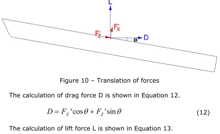
₁ ₂ ₍₁₁₎

The forces FX’ and FZ’ are relative to a coordinate system which is

relative to the trim angle of the model. The force FX’ always acts parallel to

the model baseline, while the force FX’ always acts normal to the model

baseline. To obtain the drag force D and the lift force L, FX’ and FZ’ must be

(19)

Figure 10 – Translation of forces

The calculation of drag force D is shown in Equation 12.

θ

'

sin

cos

'

Z

X

F

D

=

+

(12)

The calculation of lift force L is shown in Equation 13.

θ

'

sin

cos

'

X

Z

F

L

=

−

(13)

The pitch moment calculated in Equation 11 remain unaffected by the trim angle of the model.

In comparing hulls, drag force is of primary concern. Lift force and pitch moment are secondary and largely treated at qualitative data to inform the engineer about the characteristics of the hull form. These forces could be scaled and translated to a point on the full scale hull, but scaling data is not the focus of this research.

It should be noted that any significant lift force or pitch moment would change the running attitude of the model if it were free to move. This

would, in turn, change the drag force on the model. For this reason, this method would not be suited for hull forms which produce large amounts of dynamic lift such as planing hulls or hydrofoil craft. Using the hull geometry, weight and center of gravity of the full scale hull, one could deduce the

(20)

CHAPTER 3 – MODEL TESTS

Test Matrix

Each model was tested at two drafts to simulate two different SES air cushion modes. Full cushion corresponds to 80 percent of the ship’s

displacement supported by the air cushion, leaving 20 percent to be

supported by buoyancy. Likewise, half cushion corresponds to 40 percent of the ship’s displacement supported by the air cushion, and 60 percent

supported by buoyancy.

For each cushion mode, three trims were tested. These trims were zero degrees, one-half degree and one degree trim by the stern, which corresponds to the operating range of the full scale SES. For each cushion mode / trim combination, the models were tested at three speeds

corresponding to 20, 30 and 40 knots full scale. In total the test matrix consisted of 18 runs for each of the three hulls, or 54 runs total.

The full test matrix is attached as Appendix A.

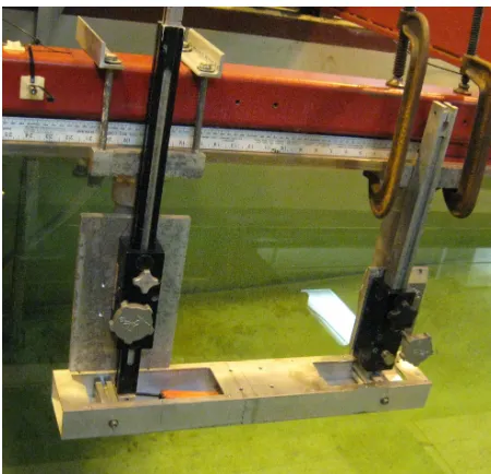
Carriage Interface

The test model and force balance were attached to the tow tank carriage via an apparatus that controls draft and trim, shown in Figure 11.

(21)

The force balance and test model mount below the horizontal box girder. Linear slides on both sides of the box girder can be adjusted by a rotary knob and lock into position allowing adjustment of draft and trim. The model is first set to the desired trim, which is measured by a digital protractor set on top of the box girder. The model is then lowered to a predetermined draft mark on the stern.

The draft for each run condition is calculated with the aid of 3-D CAD geometry. The 3-D models are rotated to the desired trim. The side hull displacement is then calculated at several draft intervals. The draft and displacement values are entered into a table, and the correct draft for the desired displacement is interpolated from this table. The test model profiles for each run condition are shown in Appendix B.

Sensor Calibration & Force Checks

Calibrating and validating the force balance used in this testing presents a unique challenge. This is due to the fact that test data is often calculated by a combination of the reading from two or all three load cells. Through some trial and error, it was found that the easiest and most

accurate method is to calibrate each load cell individually before the force balance is assembled.

After the force balance is assembled, the sensor readings are checked once again. With the force balance fixed to a solid surface, several tests are conducted to ensure that the sensors are reading properly. A pure surge force is applied to the force balance. Weights are added in even increments, and then removed one by one. Along with ensuring that the readings are correct, this test also indicates the amount of hysteresis in the system as well as the ability of the system to come back to zero when all external

forces are removed. A similar test is conducted by hanging weights from the bottom of the force balance. Hanging an identical amount of weight on both sides allows the lift force measurement to be validated, and hanging

dissimilar amounts of weight on both sides allows the pitch moment to be validated. It is also good practice to apply combinations of forces and moments to the force balance to ensure that the load cells are reading correctly.

(22)

about 1.5% of the normal force applied. The force balance is designed so that the ball transfers can be adjusted in and out towards the bottom U-channel. The optimal setting is achieved when the ball transfers are just touching the bottom U-channel. At optimal settings, there are no pre-loaded normal forces on the ball transfers, and the bottom U-channel only touches the ball transfers on one side of the force balance at any time.

The amount of drag force taken up by the friction in the ball transfers is measurable by applying a surge force with and without a sway force and measuring the difference. It turns out that this difference, within the

amount of sway force likely to be applied during testing, is within the noise range of the load cells. Therefore, it does not significantly affect the test data.

All of these calibrations and force checks take place with the force balance detached from the model. However, the force balance is checked periodically during testing by applying forces and moments directly to the model. Surge force is checked by applying weights to a string and pulley systems that is attached to the model via eyelets screwed into the deck and transom. Lift force and pitch moment are checked by placing various

(23)

CHAPTER 4 – TEST RESULTS

In the interest of simplicity, the three hull forms will from here on be referred to by the designation in Table 1.

Hull A HCAC side hull

Hull B Round Bilge side hull

Hull C Hard Chine side hull

Table 1 – Hull designations

Example Run

An example time history from a test run is shown in Figure 12. The data shown is from run 6 in the test matrix, which models hull A at full cushion, zero trim and 40 knot full scale speed.

Hull A, Full Cushion, 0 Deg Trim, 40 knots

400 450 500 550 600 650 700 750

Carriage Speed feet / second Horiz 3 lbs Vert 1 lbs Vert 2 lbs

Figure 12 – Example time history

(24)

and used to zero the data for the entire time history. This is done to calculate the dynamic lift force and pitch moment.

After the stationary section, the plot clearly shows the acceleration of the test carriage. During this time, the measure forces peak. As the

carriage reaches steady speed the forces settle down to a constant value. This is the section of the run where the data averages are taken. The plot also shows the carriage deceleration and the stationary section when the model reaches the end of the tank.

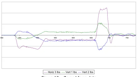
After the zeroes are applied to the time history, the data is plotted once again. This time, the carriage speed data is omitted from the plot so that the force data can be seen more clearly. An example of a zero force data plot is shown in Figure 13. This data is also from run 6.

Hull A, Full Cushion, 0 Deg Trim, 40 knots

400 450 500 550 600 650 700 750

Horiz 3 lbs Vert 1 lbs Vert 2 lbs

Figure 13 – Zeroed force data

(25)

Data Analysis

Once the averaged values have been entered into the run matrix

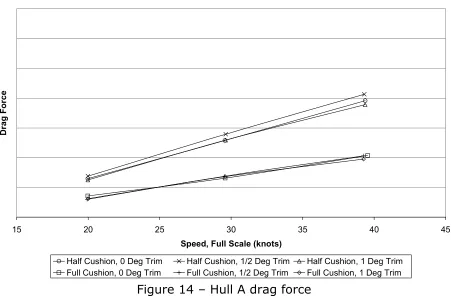
spreadsheet, equations (3) through (13) are applied to calculate the average drag force, lift force and pitch moment for the run. These averages are plotted for each hull as curves of force or moment versus full-scale speed. Separate curves are plotted for each combination of trim and air cushion condition.

The drag force data for Hull A is shown in Figure 14. Due to the proprietary nature of the data herein, ordinate values have been removed from all of the plots.

Hull A Drag Force Data

15 20 25 30 35 40 45

Speed, Full Scale (knots)

D

ra

g

F

o

rc

e

Half Cushion, 0 Deg Trim Half Cushion, 1/2 Deg Trim Half Cushion, 1 Deg Trim Full Cushion, 0 Deg Trim Full Cushion, 1/2 Deg Trim Full Cushion, 1 Deg Trim

Figure 14 – Hull A drag force

(26)

Hull B Drag Force Data

15 20 25 30 35 40 45

D

ra

g

F

o

rc

e

Figure 15 – Hull B drag force

(27)

Hull C Drag Force Data

15 20 25 30 35 40 45

D

ra

g

F

o

rc

e

Figure 16 – Hull C drag force

(28)

Hull A Lift Force Data

15 20 25 30 35 40 45

L

if

t

F

o

rc

e

Figure 17 – Hull A lift force

Hull B Lift Force Data

15 20 25 30 35 40 45

L

if

t

F

o

rc

e

(29)

Hull C Lift Force Data

15 20 25 30 35 40 45

L

if

t

F

o

rc

e

Figure 19 – Hull C lift force

Hull A Pitch Moment Data

15 20 25 30 35 40 45

P

it

c

h

M

o

m

e

n

(30)

Hull B Pitch Moment Data

15 20 25 30 35 40 45

P

it

c

h

M

o

m

e

n

t

Figure 21 – Hull B pitch moment

Hull C Pitch Moment Data

15 20 25 30 35 40 45

P

it

c

h

M

o

m

e

n

t

(31)

Comparisons

The main objective of this research is to compare multiple hull forms, so the data from all hulls must be able to be viewed simultaneously.

Additional plots were created with force or moment data of all three hulls on a single plot. As with the single hull plots, the comparative plots show the force or moment data plotted against full-scale speed. To avoid clutter, a separate plot was created for each force or moment and for each trim angle.

The drag comparison at zero trim angle is shown if Figure 23.

Drag Force Comparison, 0 Deg Trim

15 20 25 30 35 40 45

D

ra

g

F

o

rc

e

Hull A, Half Cushion Hull B, Half Cushion Hull C, Half Cushion Hull A, Full Cushion Hull B, Full Cushion Hull C, Full Cushion

Figure 23 – 0 trim drag force comparison

At half cushion, the drag curves for hulls B and C are similar at low speed. However, as speed increases, hull B shows significantly lower drag. Both hulls B and C show significantly higher drag than hull A in this

(32)

The drag comparison at ½ degree trim angle is shown in Figure 24.

Drag Force Comparison, 1/2 Deg Trim

15 20 25 30 35 40 45

D

ra

g

F

o

rc

e

Figure 24 – ½ degree trim drag force comparison

In the trimmed condition, the data looks significantly different. At half cushion, the drag curves are spaced widely apart and are roughly parallel, with hull C showing the highest drag and hull A showing the lowest. At full cushion, the drag curves for hulls B and C are very close, with hull C actually having slightly lower drag at 40 knots. Both hull B and C, however, still show higher drag than hull A.

(33)

Drag Force Comparison, 1 Deg Trim

15 20 25 30 35 40 45

D

ra

g

F

o

rc

e

Figure 25 – 1 degree trim drag force comparison

For the 1 degree trim angle, the drag curves are still widely spaced at half cushion. At full cushion, however, the drag curves are closely spaced, widening slightly at higher speeds. As before, hull C still exhibits the highest drag and hull A the lowest.

(34)

Lift Force Comparison, 0 Deg Trim

15 20 25 30 35 40 45

L

if

t

F

o

rc

e

Figure 26 – 0 degree trim lift force comparison

Lift Force Comparison, 1/2 Deg Trim

15 20 25 30 35 40 45

L

if

t

F

o

rc

e

(35)

Lift Force Comparison, 1 Deg Trim

15 20 25 30 35 40 45

L

if

t

F

o

rc

e

Figure 28 – 1 degree trim lift force comparison

The lift force data does not seem to follow any particular pattern. One notable observation is that lift force is reduced as displacement decreases for all hulls. Also, in some of the trimmed cases, the lift force is actually negative.

(36)

Pitch Moment Comparison, 0 Deg Trim

15 20 25 30 35 40 45

P

it

c

h

M

o

m

e

n

t

Figure 29 – 0 degree trim pitch moment comparison

Pitch Moment Comparison, 1/2 Deg Trim

15 20 25 30 35 40 45

P

it

c

h

M

o

m

e

n

t

(37)

Pitch Moment Comparison, 1 Deg Trim

15 20 25 30 35 40 45

P

it

c

h

M

o

m

e

n

t

Figure 31 – 1 degree trim pitch moment comparison

(38)

CHAPTER 5 – CONCLUSIONS

There is an inherent challenge in validating this test method in the context of the research presented herein. It would be desirable to compare this experimental data with analytical predictions, but one of the premises of this research was that analytical tools would not be able to fairly compare the different hull forms. Although certainly not an ideal validation method, there is some very limited analytical data that the experimental values can be compared to. As part of a related government funded project,

computational fluid dynamics (CFD) predictions were made for a subset of this test matrix. The analysis was performed with CFX, a commercial finite volume Reynolds-averaged Navier-Stokes (RANS) code which uses a volume of fluid (VOF) technique to model the free surface.

The CFD predictions were made at model scale with single side hulls. Similar to the experimental tests, the models were fixed in all degrees of freedom except for surge, and drag force, lift force and pitch moment were measured. The CFD predictions were only made for eight of the runs in the test matrix, comprised on only hulls B and C. For each hull, only four

conditions were run. The models were only run at zero and ½ degree trim, and only at combinations of 20 knots, half cushion and 40 knots full cushion.

Due to the proprietary nature of the data, the CFD predictions can only be presented here as percent differences in hulls B and C. The comparison of the CFD data and the model test data is shown in Table 1. The

percentages shown represent the increase in drag from hull B to hull C.

Case 1 2 3 4

Speed 20 knots 40 knots 20 knots 40 knots

Cushion Half Full Half Full

Trim angle 0 0 ½ by stern ½ by stern

CFD 3.2% -6.9% 2.7% -8.0%

Model test 8.5% 46.2% 16.9% 0.2%

Table 2 – Comparison of model test results to CFD predictions

This comparison ended in mixed results. In case 1, both methods indicate that the drag developed by hull C is higher, and the difference in the drag developed by the two hulls is fairly close. Case 2, however, shows no correlation between the CFD predictions and the model test results. In case 3, both methods again indicate that the drag developed by hull C is higher, but the difference is not as close as in case 1. In case 4, the CFD

(39)

The problem with this comparison is determining which method is at fault in the cases where there is a large discrepancy. The CFD method could have had problems analyzing hull C. It would likely have had problems modeling any spray phenomenon caused by the hard chine hull. If spray drag was not correctly accounted for, then the CFD method would under-predict the drag in hull C. However, although this hypothesis is consistent with the data shown in Table 2, it is unlikely that spray drag could account for such a large difference. Errors in the model test method could just as likely be guilty of the discrepancy.

The fact that hull B and C showed consistently higher drag than hull A was expected. The fine lines and tapered stern of the HCAC hull usually produce favorable performance, especially at lower speeds. However, it was unexpected that hull C did not perform better at higher speeds. Data from the Textron Marine & Land library shows that traditional hard chine SES hull forms usually outperform round bilge types at higher speeds. Once again, the test data presented here is not conclusive enough to determine if this is due to the test method, or if is an actual physical phenomenon.

It should be noted that data repeatability in these tests was

satisfactory. Although not every run was checked, the handful that were showed very close agreement in the data. An example of a repeated run is shown in shown in Figure 32.

Run 3 Repeated

-1 -0.5 0 0.5 1 1.5

(40)

Figure 32 shows two time histories from run 3 overlaid on the same graph. The time histories had to be shifted on the abscissa to occupy the same time region. The graph shows that the measure force data was very close in these two runs. In fact, the difference in the averaged drag data was less than one percent.

Recommendations

The objective of the research presented herein was to find an economical method of comparing multiple hull forms. In the author’s opinion, this research was inconclusive in reaching this goal. Further

validation must occur to determine if this is a feasible and trustworthy test method.

The most accurate way to validate this test method would most likely be to test multiple hulls that could be analyzed with a single analytical tool. For instance, several variations on a simple displacement type hull could be model tested. These same hulls could then be accurately analyzed with CFD tools, resulting in a straightforward comparison of data. A similar

comparison could be made with variations on a planing hull. An analytical tool specifically designed to analyze planing hulls could then be used to validate the data. This test would also indicate if this test method is a fair way to compare hull forms that generate dynamic lift.

(41)

APPENDIX A – TEST MATRIX

1 A 40% 0 8.7 20 4.36

2 A 40% 0 8.7 30 6.54

3 A 40% 0 8.7 40 8.72

4 A 80% 0 3.3 20 4.36

5 A 80% 0 3.3 30 6.54

6 A 80% 0 3.3 40 8.72

7 A 40% 0.5 9.6 20 4.36

8 A 40% 0.5 9.6 30 6.54

9 A 40% 0.5 9.6 40 8.72

10 A 80% 0.5 4.2 20 4.36

11 A 80% 0.5 4.2 30 6.54

12 A 80% 0.5 4.2 40 8.72

13 A 40% 1 10.5 20 4.36

14 A 40% 1 10.5 30 6.54

15 A 40% 1 10.5 40 8.72

16 A 80% 1 5.0 20 4.36

17 A 80% 1 5.0 30 6.54

18 A 80% 1 5.0 40 8.72

19 B 40% 0 7.8 20 4.36

20 B 40% 0 7.8 30 6.54

21 B 40% 0 7.8 40 8.72

22 B 80% 0 3.1 20 4.36

23 B 80% 0 3.1 30 6.54

24 B 80% 0 3.1 40 8.72

25 B 40% 0.5 8.7 20 4.36

26 B 40% 0.5 8.7 30 6.54

27 B 40% 0.5 8.7 40 8.72

28 B 80% 0.5 3.9 20 4.36

29 B 80% 0.5 3.9 30 6.54

30 B 80% 0.5 3.9 40 8.72

31 B 40% 1 9.4 20 4.36

32 B 40% 1 9.4 30 6.54

33 B 40% 1 9.4 40 8.72

34 B 80% 1 4.6 20 4.36

35 B 80% 1 4.6 30 6.54

36 B 80% 1 4.6 40 8.72

37 C 40% 0 8.3 20 4.36

38 C 40% 0 8.3 30 6.54

39 C 40% 0 8.3 40 8.72

40 C 80% 0 3.6 20 4.36

41 C 80% 0 3.6 30 6.54

42 C 80% 0 3.6 40 8.72

43 C 40% 0.5 9.1 20 4.36

44 C 40% 0.5 9.1 30 6.54

45 C 40% 0.5 9.1 40 8.72

46 C 80% 0.5 4.2 20 4.36

47 C 80% 0.5 4.2 30 6.54

48 C 80% 0.5 4.2 40 8.72

49 C 40% 1 9.9 20 4.36

Trim by Stern (deg)

Draft reading at stern (ft - FS)

Speed (ft/s - MS)

Run Hull % ∆ supported

by cusion

(42)

APPENDIX B – TEST MODEL PROFILES

Hull A, Half Cushion

0 Deg Tr im

½ Deg Trim

1 Deg Trim

Hull A, Full Cushion

0 Deg Tr im

½ Deg Trim

(43)

Hull B, Half Cushion

0 Deg Tr im

½ Deg Trim

1 Deg Trim

Hull B, Full Cushion

0 Deg Tr im

½ Deg Trim

(44)

Hull C, Half Cushion

0 Deg Tr im

½ Deg Trim

1 Deg Trim

Hull C, Full Cushion

0 Deg Tr im

½ Deg Trim

(45)

Comparative Hydrodynamic Testing of Small Scale Models

ScholarWorks@UNO

ScholarWorks@UNO

Comparative Hydrodynamic Testing of Small Scale Models

Comparative Hydrodynamic Testing of Small Scale Models

TABLE OF CONTENTS

LIST OF TABLES

LIST OF FIGURES

NOTATION

ABSTRACT

INTRODUCTION

CHAPTER 1 – TEST MODELS

gL

V

F

=

λ

V

V

=

CHAPTER 2 – FORCE BALANCE

0

=

∑

F

0

'

−

=

R

F

R

F

'

=

0

=

∑

F

0

'

+

+

=

R

R

F

'

R

R

F

=

−

−

0

=

∑

M

0

2

2

'

+

R

l

−

R

l

+

R

h

=

M

(

R

R

)

l

R

h

₋

₌

₊

₊

₌

₊

_R

₋

_R

₊

_R

_h

₌