Implementing some mathematical operators for a continuous-in-time financial model

Eng. Math. Lett. 2017, 2017:2 ISSN: 2049-9337

IMPLEMENTING SOME MATHEMATICAL OPERATORS FOR A CONTINUOUS-IN-TIME FINANCIAL MODEL

TARIK CHAKKOUR

Univ. Bretagne-Sud, UMR 6205, LMBA, F-56000 Vannes, France

Copyright c2017 Tarik Chakkour. This is an open access article distributed under the Creative Commons Attribution License, which permits

unrestricted use, distribution, and reproduction in any medium, provided the original work is properly cited.

Abstract. This paper considers the development of some mathematical operators as convolution and primitive

for continuous-in-time financial model. This development is given in form of API (Application Programming

Interface) with showing concept of its computation. The model is based on using measures and fields. The work

we report here addresses the fundamental issue of how measures and fields are implemented for the software. The

originality of this API lie in the fact that it will be used by the company MGDIS.

Keywords:API; convolution; primitive; discretization; integration; software tool.

2010 AMS Subject Classification:34A45, 65M22, 68N30.

1. Introduction

Time is the central element that influence financial economic behavior. The time financial model constitutes a powerful tool for studying the development of continuous-in-time methods in finance. We refer to papers [1, 2], which are dealing with continuous-in-continuous-in-time financial model. These papers develop the mathematics and economic theory of finance from the perspective of a model in which agents can revise their decisions continuously in time. At the same time, we have seen an explosion in the use of algorithms for computation methods to

Received November 29, 2016

implement continuous-time models. The covered methods include convolution and primitive has been one of the most effective and widely-used of these methods. They began to be studied and applied systematically in various branches of modern science as in finance. We refer to [3] that presents an approach for implementing continuous-time adaptive recursive filters for convolution operator.

Within this paper, SOFI [4] is a software tool marketed by the company MGDIS. It is de-signed to the public institutions such local communities to set out multiyear budgets. SOFI is based on a discrete financial modeling. Currently, the mathematical objects involved in SOFI are suites and series. The discrete model generates outcomes in the form of tables. We showed in previous work [5] the default of this discrete model. We build a new model with using an other paradigm in [5]. This new model is based on continuous-in-time model and uses the mathematical tools such convolution and integration to describe loan scheme, reimbursement scheme and interest payment scheme. In [6] we have shown some results about improving one of the continuous-in-time financial models built in paper [5]. We use in [6] a mathematical framework to discuss an inverse problem of the continuous-in-time model.

This article describes implementing the continuous-in-time financial model. Mainly, we fo-cus on concept of computation in API. This API is to be integrated in SOFI in order to produce the continuous software, and is restricted to certain measures and fields. The purpose of com-puting integration of measures over a time interval is to compute loan scheme, reimbursement scheme, etc; and the purpose of computing evaluation of fields at an instant is to compute cur-rent debt amount, where curcur-rent debt field is a function that, at any time t, gives the capital amount still to be repaid.

repayment measure with the Fast Fourier Transform method. We use primitive to compute cur-rent debt field at an instantt with accumulating measures between initial time and timet. The primitive of measure is defined as a field in spite of it is undefined in the Radon measure space. In this work, we describe how we impelement and check these operators.

The rest of this paper contains three sections. The first one introduces time steps that are involved in the models in order to show concept of computation in API. In the second we review numeric choices linked to API, where we define a field as continuous function by superior value. The last one shows implementation details about convolution and primitive.

2. Concept of computation in API

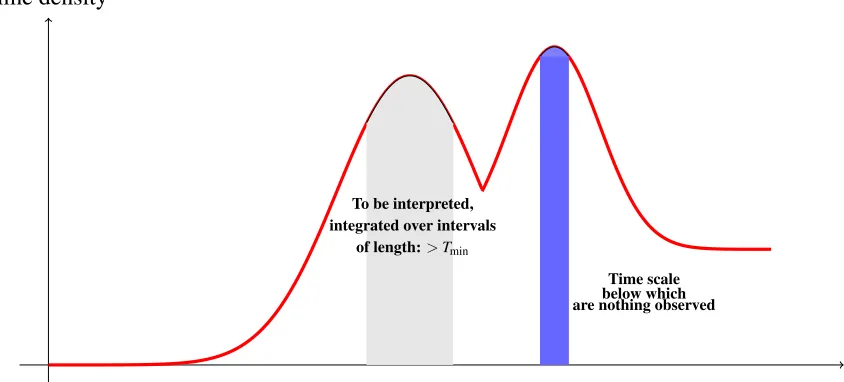
This section is devoted to explain time steps that are involved in the model and the relations between them. We give the time scales to integrate measure over interval which are shown in Figure 1. We introduce T_min which is the time scale below which nothing coming from the model will be observed. To be more precise, we say that a measure ˜mis observed over time interval[t1,t2]if

Z t₂

t1

˜

m, (2.1)

is computed. And, we will always, choose timest₁andt₂such thatt₂−t₁>T_min. In order to ob-serve models, we need an observation stepT_obswhich is strictly superior to minimal observation stepT_min

T_obs>T_min. (2.2)

We define the discrete stepTdMas a smaller step than stepTminto discretize measures:

T_dM≤T_min. (2.3)

For instance, we are setting discrete stepT_dMby following equality:

T_dM= Tmin

Observation stepT_obsis partitioned inton_Ddiscrete stepT_dMdefined by:

n_D=

"

T_obs T_dM

#

. (2.5)

A field is evaluated between inferior valueaand superior valuebwith discrete stepT_dF satisfy-ing:

T_dF<b−a. (2.6)

Since measures and fields compose API, they are shared in two levels which are shown in Figure 2. First is high level and is created for business reasons. The computation in high level is designed to the SOFI users. Second is low level which is only used by the high level. The computation in low level is designed to the high level users. Notice that low level doesn’t use its high. We say that high level implements its low. High and low levels contain non-discrete measures, non-non-discrete fields defined on_R, discrete measures and discrete fields. Some computations in high level need discretization. For instance, if we want to discretize a measure in high level, we create its copy in low level. Then we discretize it in order to rise up its values to high level.

Time density

Time scale To be interpreted, integrated over intervals

of length:>Tmin

Time scale below which are nothing observed

The aim here is to explain how measures are integrated and how fields are evaluated. A non-discrete measure in low level is integrated between inferior boundaand superior boundbwith minimal observation step T_min and observation step T_obs. It follows that discrete step T_dM is computed with relation (2.4). Whereas in high level it is integrated between inferior boundsa and superior boundb. A non-discrete field in low level is evaluated between inferior valueaand superior valueb with discrete stepT_dF. Yet, its evaluation in high level is done only between inferior valueaand superior valueb.

The parallelism of discrete measures and fields in low level is based on the concept of a task. Tasks provide much benefits: more efficient computation and robustness API. Precisely, the Task Parallel Library [7] is used to entail execution and development speed. It is shown in [8] that this library makes it easy to take advantage of potential parallelism in a program. It relies heavily on generics and delegate expressions. Paper [9] shows several strategies that can be applied in large-scale discrete distribution clustering tasks.

In what follows, we build the unidimensional mesh called DAS (DiscretizedAxeSegment presented in Figure 3) for two reasons. First is to better structure the low level. Second is to compute discrete convolution due to the impossibility for computing it with variable step using the Fast Fourier Transform. Mesh DAS associated to discrete step T_dM is defined by a set of points(x_k)_k∈

Z that are its multiple

DAST_dM={x_k=k×T_dM,k∈_Z}. (2.7) Integration of measure m_d in low level between inferior bound a and superior bound b with minimal observation stepT_min returns its integration between new inferior bound x_a and new superior boundx_bwith discrete stepT_dM, where

x_a=n_a×T_dM, (2.8)

such that:

n_a=

"

a T_dM

#

, (2.9)

x_b=n_b×TdM, (2.10) such that:

n_b=



     

     

b

TdM if TdM is divisible by b, "

b T_dM

#

+1 else.

(2.11)

High level

Low level SOFI

Lemf (Library Embedded Finance)

LemfAN (Library Embedded Finance And Numerical Analysis)

API

FIGURE 2. API composition.

−∞ •a •b +∞

x_a x_b

• • • • • • • • •

FIGURE 3. Mesh DAS defined on_R.

Interval[xa,xb]is partitioned intoNabsubintervals of equal length, whereNabis given by:

N b

discrete value, the integration of measure m_d between inferior bound (n_a+ j−1)×T_dM and superior bound(na+ j)×TdMgiven by following equality:

∀j∈[[1;N_ab]],m_d(na+j−1) =

Z (na+j)×T_dM

(na+j−1)×TdM

m_d. (2.13)

For any integerifrom 1 to

"

N b a n_D

#

, we define quantitymobs_d (i)as observed measure over time interval that its length is T_obs between inferior bound n_a×T_dM+ (i−1)×T_obs and superior boundn_a×T_dM+i×T_obs. Formally,mobs_d (i)is defined as:

∀i∈

"" 1; " N b a n_D ###

,mobs_d (i) =

Z na×T_dM+i×T_obs

na×TdM+(i−1)×Tobs

m_d, (2.14)

which is decomposed with Chasles relation as:

∀i∈

"" 1; " N b a n_D ###

,mobs_d (i) = nD

∑

Z (na+k−n_D)×T_dM+i×T_obs

(na+k−1)×TdM+(i−1)×Tobs

m_d. (2.15)

Because of (2.5) and of the fact thatl=k+ (i−1)×n_D, relation (2.15) implies that:

∀i∈

"" 1; " N b a n_D ###

,mobs_d (i) =

i×nD

∑

Z (na+l)×T_dM

(na+l−1)×TdM

m_d. (2.16)

From this and according to (2.16), we conclude that observed valuemobs_d (i)is a sum of values m_d(na+l−1)for integerlfrom 1+ (i−1)×nDtoi×nD

∀i∈

"" 1; " N b a nD ###

,mobs_d (i) =

i×nD

∑

m_d(na+l−1). (2.17)

There are two situations for computing observed values. IfN_abis divisible byn_D, then

"

N b a n_D

#

observed values are computed with relation (2.17). Else,

"

N b a nD

#

observed values are

com-puted with relation (2.17) such that the observed value mobs_d

" N b a n_D # +1 !

mobs_d

"

N b a n_D

#

+1

!

=

Nb

a

∑

k=nD×

"

Nb a nD

#

+1

m_d(na+k−1). (2.18)

3. Numeric choices in API

We are concerned in this section about implementation choices providing for great flexibility in API. Given a continuous functionφ, the Dirac measure δp at point p acts on the function

φ. The value of this action is φ(p). The purpose is to maintain this action in API. For that,

we will explain the numeric choices that we have made to achieve it due to the difficulty for describing the dual of vector space of continuous piecewise function with a finite number of pieces, continuous with superior values. For instance, the action of Dirac measureδp on fields

1]−∞,p]and1[p,+∞[is undefined. Indeed, they integrals with respect to Dirac measureδpcould not be computed. Formally, following integrals

Z +∞

−∞

1]−∞,p]dδp(x),

Z +∞

−∞

1[p,+∞[dδp(x), (3.1) are undefined. In order to set the value of this action consistently, we make a choice on Dirac measureδpdefined by:

<δp,φ >= lim

x→p+φ(x). (3.2)

Consider a continuous functiong with integral equals 1 over _R. To justify relation (3.2), we may restrict to support of functiongdefining functiong_ε which approaches Dirac measureδp,

and is defined as:

gε(x) =

1

εg

x−p

ε +εp !

. (3.3)

g

x p(1+ε2)

FIGURE 4. Restriction to support of functiongdefining functiong_ε in relation (3.3).

lim

ε→0+

g_ε=δp. (3.4)

To obtain relation (3.2), we require the following inclusion:

Supp(gε)⊂]p,+∞[, (3.5)

because of:

Supp(g)⊂]p,+∞[. (3.6)

Relation (3.6) provides restriction to support of functiongillustrated in Figure 4 due to follow-ing equivalence:

∀ε∈_R∗₊,x> p ⇐⇒ 1 ε ×

x−p

ε +εp !

>p. (3.7)

4. Convolution and accumulation

numerical errors of discrete FFT. In the model, Loan Measure ˜κEis defined such that the amount borrowed between timest₁andt₂is:

Z t₂

t1

˜

κE, (4.1)

and Repayment Measure ˜ρ_K is defined such that the amount borrowed between timest1andt2 is:

Z t₂

t1

˜

ρ_K. (4.2)

Loan Measure ˜κE and Capital Repayment Measure ˜ρK are connected by a convolution oper-ator. It is required to implement it in order to compute repayment amount. Then the discrete convolution may be evaluated with the aid of FFT method. By the Fourier convolution theorem, the discrete Fourier transform of ˜κE?γ˜may be computed as

F(ρ˜_K) =F(κ˜E?γ˜) =F(κ˜E)•F(γ˜), (4.3) where the Repayment Pattern Measure ˜γ expresses the way an amount 1 borrowed at t =0

is repaid and where • denotes component-wise multiplication. QuantitiesF(κ˜E) and F(γ˜)

define discrete Fourier transforms of ˜κE and of ˜γ, respectively. The computation of discrete convolution (κ˜E?γ˜(ne+j−1))_1≤j≤N f

e with discrete measures (κ˜E(na+j−1))1≤j≤Nab and (γ˜(nc+ j−1))1≤j≤Nd

c between pointsxe andxf of universel mesh DASTdM is summarized as follows:

• Determine the convex hull of the support of discrete measure(κ˜E(na+j−1))1≤j≤Nb a supposed to be interval[xa1,xb1];

• Determine the convex hull of the support of discrete measure (γ˜(nc+ j−1))1≤j≤Nd c supposed to be interval[x_c1,x_d1];

• Complete by zero discrete measures(κ˜E(na+j−1))1≤j≤Nb

a and(γ˜(nc+j−1))1≤j≤Ncd such that they have N values, where N is power of 2 and is smallest value satisfying

N≥N b

• Compute discrete measures(x(n_a+ j−1))_1≤j≤N and(y(n_c+ j−1))_1≤j≤N by Fourier transform of discrete measures (κ˜_E1(na+ j−1))1≤j≤N and (γ˜1(nc+j−1))1≤j≤N, re-spectively;

• Compute vector z(j−1)1≤j≤N defined by element-wise multiplication of (x(na+ j− 1))1≤j≤N by(y(nc+j−1))1≤j≤N;

• Compute vector(h(j−1))1≤j≤Ndefined by inverse Fourier transform of(z(j−1))1≤j≤N;

• Build tabulated measure ˜m_Tabulated between inferior value xa1+xc1 and superior value

x_b1+x_d1 with a set of firstN_ab+N_cd values ofh;

• Discretize tabulated measure ˜m_Tabulatedbetween pointsxeetxf with discrete stepTdMto get discrete values(κ˜E?γ˜(ne+ j−1))_1≤j≤N f

e .

The integration of discrete measure(κ˜E?γ˜(ne+j−1))_1≤j≤N f

e in high level between inferior boundeand superior bound f is the sum of its values given by:

N f

e

∑

˜

κE?γ˜(ne+j−1).

After defining convolution operator, we describe how the accumulation of measure is defined in API. The Current Debt FieldKRDis related to Loan Measure ˜κE and Repayment Measure ˜ρ_K

by the following Ordinary Differential Equation:

dKRD

dt =κE(t)−ρK(t). (4.4)

The solution of this ODE is expressed:

KRD(t) =KRD(tI) + Z t

tI

˜

κE−

Z t

tI

˜

ρ_K. (4.5)

superior valuex_b with discrete stepT_dF is defined by discrete field(F_dD(na+k−1))1≤k≤Nb a+1 given by:

∀k∈[[1;N_ab+1]],F_dD(na+k−1) =

Z y_k

xc

m_d, (4.6)

where points(yk)1≤k≤Nb

a +1are defined as:

∀k∈[[1;N_ab+1]],y_k=xa+ (k−1)×TdF. (4.7) We distinguish three cases of computing discrete field(F_dD(na+k−1))1≤k≤Nb

a +1:

First casexc<xa

Measurem_d is discretized between pointsxc andxb with discrete stepTdF to compute discrete measure (md(nc+j−1))1≤j≤Nb

c . The integral defined in relation (4.6) is decomposed with Chasles relation to get:

∀k∈[[1;N_ab+1]],F_dD(na+k−1) =

Na

c

∑

Z xc+j×T_dF

xc+(j−1)×TdF

m_d+ k−1

∑

Z xa+j×T_dF

xa+(j−1)×TdF

m_d. (4.8)

Replacingxabyxc+Nca×TdFin relation (4.8), we obtain the following equality:

∀k∈[[1;N_ab+1]],F_dD(na+k−1) =

Na

c

∑

Z xc+j×T_dF

xc+(j−1)×TdF

m_d+ k−1

∑

Z xc+(j+N_ca)×T_dF

xc+(j−1+Na c)×TdF

m_d. (4.9)

From this and using relation (2.13) which defines discrete measure, we get:

∀k∈[[1;N_ab+1]],F_dD(na+k−1) =

Na

c

∑

m_d(nc+j−1) +

k−1+Na c

∑

c

m_d(nc+j−1). (4.10)

Measure m_d is discretized between points x_a and x_c with discrete step T_dF to compute dis-crete measure(md(na+j−1))1≤j≤Nc

a . It follows that Chasles relation applied to relation (4.6) gives:

∀k∈[[1;N_ab+1]],F_dD(na+k−1) =−

Nc

a

∑

Z xa+j×T_dF

xa+(j−1)×TdF

m_d, (4.11)

which is reduced to following equality:

∀k∈[[1;N_ab+1]],F_dD(na+k−1) =−

Nc

a

∑

m_d(na+j−1). (4.12)

Third casex_a≤x_c≤x_b

Determining integerL∈[[1;N_ab]]satisfying following inequalities:

y_L<x_c≤y_L+1. (4.13)

Sincex_c>y_kfor each integerkfrom 1 toL, the result of second case implies that:

∀k∈[[1;L]],F_dD(na+k−1) =−

Nc

a

∑

m_d(na+ j−1). (4.14)

Replacingx_cbyx_a+N_ac×T_dFin relation (4.6) and employing Chasles relation, we obtain:

∀k∈[[L+1;N_ab+1]],F_dD(na+k−1) = k−1

∑

a

m_d(na+ j−1). (4.15)

Conflict of Interests

The authors declare that there is no conflict of interests.

REFERENCES

[1] R.C. Merton, Theory of finance from the perspective of continuous time, Journal of Financial and Quantitative

Analysis, 10(04) (1975), 659-674.

[3] D. Johns, W.M. Snelgrove, A.S. Sedra, Continuous-time lms adaptive recursive filters. IEEE Transactions on

Circuits and Systems, 38(7) (1991), 769-778.

[4] SOFI, https://www.mgdis.fr/index.phppage=display doma&class=article&object=sol sofi programmation

financiere&method=display full&refo=001009, Accessed: 2016-08-16.

[5] E. Fr´enod, T. Chakkour, A continuous-in-time financial model. Mathematimathcal Finance Letters, 2016

(2016), Article ID 2.

[6] T. Chakkour, E. Fr´enod, Inverse problem and concentration method of a continuous-in-time financial model,

International Journal of Financial Engineering, 3(2) (2016), 1650016-1650036.

[7] Task parallel library [online], https://msdn.microsoft.com/fr-fr/library/dd537609%28v=vs.110%29.aspx,

Ac-cessed: 2016-06-30.

[8] D. Leijen, W. Schulte, S. Burckhardt, The design of a task parallel library, Acm Sigplan Notices, 44(10)

(2009), 227-242.

[9] Y. Zhang, J.Z. Wang, J. Li, Parallel massive clustering of discrete distributions, ACM Trans. Multimedia

Comput. Commun. Appl., 1 (1) (2015), Article ID 1.

[10] T. Hearn, L. Reichel, Fast computation of convolution operations via low-rank approximation, Applied

Nu-merical Mathematics, 75 (2014), 136-153.

[11] T. Tanaka, I. Tomohiro, S. Inenaga, H. Bannai, M. Takeda, Computing convolution on grammar-compressed

text, In Data Compression Conference (DCC), IEEE, (2013), 451-460.

[12] P. Schaller, G. Temnov, Efficient and precise computation of convolutions: applying fft to heavy tailed

distri-butions Computational Methods in Applied Mathematics Comput, Methods Appl. Math., 8(2) (2008),