Evaluation of Substructure Reduction Techniques with Fixed and Free Interfaces

0 INTRODUCTION

Nowadays the increasing performance of modern computers makes it possible to solve very large linear systems of millions of degrees of freedom (DOF). Nevertheless, since dynamic analysis requires solving a lot of linear systems and since the refinement of finite element models is increasing faster than the computing capabilities, dynamic substructuring still remains an essential tool for analyzing dynamical systems in an efficient manner. Building reduced models of subparts of a structure enables sharing models between design groups. Moreover the reduction of the DOF of substructures is also important for building reduced order models for optimization and control. If a single component of a system is changed, only that component needs to be reanalyzed and the system can be analyzed at low additional cost. Thus dynamic substructuring offers a flexible and efficient approach to dynamic analysis.

Dynamic substructuring techniques can be classified in two categories depending on the

underlying modes which are used [1]. The term mode

can refer to all kind of structural shape vectors. The

first class consists of methods using fixed interface vibration modes and interface constraint modes to represent the substructure dynamics. The method commonly used is the Craig-Bampton method (CBM)

[2] which assembles the substructures in a primal

way using interface displacements in order to enforce interface compatibility. The second class consists of methods using free interface vibration modes and attachment modes. Common representatives

of that class are MacNeal‘s method (MNM) [3] and

Rubin‘s method (RM) [4] using a primal assembly

process as well. Herting generalizes in [5] the concept

of component mode synthesis to include any kind of interface boundary condition for the modes. In contrast to the aforementioned methods, the dual

Craig-Bampton method (DCBM) [6] uses the same

ingredients as MacNeal‘s and Rubin‘s method, but assembles the substructures in a dual way using interface forces. As a consequence, the DCBM enforces only weak interface compatibility between the substructures, thereby avoiding interface locking problems as sometimes experienced in the primal assembly approaches. Furthermore, the dual Craig-Bampton method leads to simpler reduced matrices

Evaluation of Substructure Reduction Techniques

with Fixed and Free Interfaces

Gruber, F.M. – Rixen, D.J.

Fabian M. Gruber* _{– Daniel J. Rixen}

Technical University of Munich, Institute of Applied Mechanics, Germany

Substructure reduction techniques are efficient methods to reduce the size of large models used to analyze the dynamical behavior of complex structures. The most popular approach is a fixed interface method, the Craig-Bampton method (1968), which is based on fixed interface vibration modes and interface constraint modes. In contrast, free interface methods employing free interface vibration modes together with attachment modes are also used, e.g. MacNeal‘s method (1971) and Rubin‘s method (1975). The methods mentioned so far assemble the substructures using interface displacements (primal assembly). The dual Craig-Bampton method (2004) uses the same ingredients as the two aforementioned free interface methods, but assembles the substructures using interface forces (dual assembly). This method enforces only weak interface compatibility between the substructures, thereby avoiding interface locking problems as sometimes experienced in the primal assembly approaches using free interface modes. The dual Craig-Bampton method leads to simpler reduced matrices compared to other free interface methods and the reduced matrices are sparse, similar to the classical Craig-Bampton matrices. In this contribution we evaluate the primal (classical) formulation of the Bampton method, the MacNeal method, the Rubin method and the dual formulation of the Craig-Bampton method. The presented theory and the comparison between the four substructuring methods will be illustrated on the Benfield truss, on a three-dimensional beam frame and on a two-dimensional solid plane stress problem.

Keywords: dynamic substructuring, component mode synthesis, model order reduction, dual assembly, Craig-Bampton method, free interface method

Highlights

• Derivation of the Craig-Bampton, MacNeal, Rubin and dual Craig-Bampton method in a common framework. • Highlighting the differences and emphasizing the similarities between the four methods.

• Assessing the accuracy of the methods.

• Evaluation of the sparsity pattern of the reduced matrices.

compared to other free interface methods and the reduced matrices are sparse, similar to the classical Craig-Bampton matrices. In this contribution we evaluate the primal (classical) formulation of the Craig-Bampton method, the MacNeal method, the Rubin method and the dual formulation of the Craig-Bampton method. The presented theory and the comparison between the four substructuring methods will be illustrated on three different examples.

In section 1, the differences between primal and dual assembly are stated. Following this, the formulation of the CBM, the MNM, the RM and the DCBM will be outlined in section 2 explaining general properties of the fixed interface method (subsection 2.1) and of the free interface methods (subsection 2.2). These properties will be illustrated subsequently in detail in section 3 using the Benfield Truss (subsection 3.1), a three-dimensional beam frame (subsection 3.2) and a two-dimensional solid plane stress problem (subsection 3.3). Finally a brief summary and conclusions are given in section 4.

1 PRIMAL AND DUAL ASSEMBLY OF SUBSTRUCTURES

Consider a finite element model of a global domain.

This domain is divided into N non-overlapping

substructures such that every node belongs to exactly one substructure except for the nodes on the interface boundaries. The linear/linearized equation of motion of one substructure is written as

M( ) ( )s _�u_s ₊K u( ) ( )_�s s ₌ f( )s ₊g( )s _{, (1)}

where the superscript (s) is the label of the particular substructure

(

)

the mass matrix, the stiffness matrix and the displacement vector of the substructure, respectively.

f( )s _{is the external force vector and g}( )s _{is the vector}

of reaction forces on the substructure due to its connection to adjacent substructures at its boundary

DOF. The local displacements u( )s _{of each}

substructure can be divided in local internal DOF u_i( )s and boundary DOF ub( )s :

u u u L I u u

s bs

is

bs b

is ( ) ( ) ( ) ( ) ( ) =       =              0

0 . (2)

The boundary DOF u_bs L u

bs b

( )₌ ( ) _{of the}

substructure are a subset of the assembled boundary

DOF u_b of the global domain. L( )bs is a Boolean

localization matrix (connectivity matrix) relating the

assembled boundary DOF u_b of the global domain to

the substructure boundary DOF ub( )s . Consequently,

the equation of motion, Eq. (1), of one substructure partitioned in the same manner writes

M M

M M

K u

u

bbs bis

ibs iis bs is bb ( ) ( ) ( ) ( ) ( ) ( )                +   ss bis

ibs bbs bs is bs is ( ) ( ) ( ) ( ) ( ) ( ) ( )                = = K K K u u f

f(( )

( )        +      

gbs

0 . (3)

Defining the local Boolean localization matrix

A( )s _{which is selecting the boundary DOF of}

substructure s gives the relation

u_b( )s ₌A u( ) ( )s s _{, (4)}

which will be used later.

1.1 Primal Assembly

The Eqs. (1) and (2) of all substructures N can be

assembled in a primal way as:

Ma au +K ua a= fa, (5)

where

M

M M M

M M �

� �

M � M

a

bb bi biN

ib ii ib N ii N = ( ) ( ) ( ) ( ) ( ) ( ) 1 1 1 0 0                

, (6)

K

K K K

K K �

� �

K � K

a

bb bi bi

N

ib ii

ibN iiN

= ( ) ( ) ( ) ( ) ( ) ( ) 1 1 1 0 0                

, (7)

u u u u f f f f a b i iN a b i iN =               =           ( ) ( ) ( ) ( ) 1 1 , _  

, (8)

with

M L M L

M M L M L M

bb s

N

bs bbs bs

ib _ibs _bs bi _bs _b

T T = = = = ( ) ( ) ( ) ( ) ( ) ( )

∑

, _iis

bb s

N

bs bbs bs

ib _ibs _bs bi _b

T ( ) = ( ) ( ) ( ) ( ) ( ) = = =

∑

K L K L

K K L K L

1 ss bis b s N bs bs

T T ( ) ( ) = ( ) ( ) =

∑

f L f

,

1

The reaction forces g( )s _{on the interfaces of the}

substructures cancel out during assembly. This assembly is called primal assembly since the compatibility between the substructures is enforced using the same boundary displacements for adjacent substructures.

1.2 Dual Assembly

Another way to enforce the interface compatibility between the substructures is to consider the interface connecting forces as unknowns. These forces must be determined to satisfy the interface compatibility condition (displacement equality) and the local equation of motion of the substructures:

B us s s

N ( ) ( )

= =

∑

M u_{( ) ( )}s s K u_{( ) ( )}s s B_{( )}sT f_{( )}s

+ + =

 λλ . (10)

B( )s _{is a signed Boolean matrix (constraint matrix)}

acting on the substructure interface DOF. B_{( )}sT

λλ is representing the interconnecting forces between substructures which is corresponding to the negative interface reaction force vector g( )s _{in Eq. (1) meaning}

gs Bs g B

bs bs

T T

( )_{= −} ( )_λλ, ( )_{= −} ( )_{λλ, (11)}

and λλ is the vector of all Lagrange multipliers acting on the interfaces which are the additional unknowns.

The displacement vector u( )s _{is partitioned according}

to Eq. (2). With the block-diagonal matrices

M M

M

= 

   



   

( )

( )

1 0

0



N

, (12)

K K

K

= 

   



   

( )

( )

1 0

0



N

, (13)

and

u u

u f

f

f

= 

   



  

 =



   



   

( )

( )

( )

( )

1 1

 

N N

, , (14)

B_{= }B( )1 B( )_

 N _{, (15)}

the set of Eqs. (9) and (10) can be written as:

M u K B

B

u f

0

0 0 0 0

 

 

 

  

  +



 

 

  

  =

  

 

 

λλ λλ

T

(16)

In this hybrid formulation the Lagrange

multipliers λλ enforce the interface compatibility

constraints and can be identified as interface forces [6]. The dual assembled system in Eq. (16) is equivalent to the primal assembled system in Eq. (5) since both systems express the same local equilibrium for each substructure and enforce the same interface compatibility.

2 COMPONENT REDUCTION METHODS

2.1 Craig-Bampton Method (CBM)

Considering the partitioned equation of motion in Eq. (3), the internal DOF ui( )s of every substructure can be seen as being excited by its boundary DOF

ub( )s , namely

Mii( ) ( )suis +K uii( ) ( )s is = fi( )s −K uib( ) ( )s bs −Mib( ) ( )subs . (17)

This indicates that ui( )s of each substructure can be approximated by a superposition of a static

response and of eigenmodes associated to Mii( )s and

K_ii( )s _{. The static response is given by}

u_{i stat}s K K u u

iis ibs bs ibs bs ,

( ) _{= −} ( )−1 ( ) ( )₌ ( ) ( )

Ψ

Ψ , (18)

where the columns of matrix ΨΨ_ib( )s _{are the static}

response modes also called constraint modes [2]. The

fixed interface normal modes φφ( )_ks _{are obtained as}

eigensolutions of the generalized eigenproblem

Kii( ) ( )sφφks =ωk( )s Mii( ) ( )sφφks

2

. The columns of the

ni( )s ×nφ( )s matrix ΦΦiφ( )s contain the first nφ( )s fixed

interface normal modes φφ_k( )s _{which can also be}

considered as the free vibration modes of the substructure s clamped on its boundary DOF ub( )s . The approximation of ui( )s therefore writes

u_is u

i stats is s

( )_≈ ( ) ₊ ( ) ( )

, ΦΦφηη , (19)

and the displacements of the substructure are approximated by

u u

I u

bs

is

bbs bs

ibs is bs

s ( )

( )

( ) ( )

( ) ( )

( )



  



  =



  



  

0φ

φ Ψ

Ψ ΦΦ ηη(( ) 

  



 

, (20)

with the vector of modal parameters ηη( )s _{of dimension} ns

φ( ) corresponding to the amplitudes of the fixed

interface normal modes ΦΦ_is

φ

( )_{. The CBM reduction}

matrix TCB for reducing the primal assembled system

u

I L

L

a ib b i

ibN bN iN

≈              ( ) ( ) ( ) ( ) ( ) ( ) 0 0 0 0 Ψ Ψ ΨΨ ΦΦ Φ Φ

1 1 1

φ φ                ( ) ( ) T u CB b N ηη ηη 1

, (21)

and the CBM reduced matrices

K_{red CB} T K T_CBT a CB

, = , (22)

M_{red CB} T M T_CBT a CB

, = , (23)

are found in [2].

2.2 Free Interface Methods

Considering the equation of motion (Eq. (10)) of

substructure s, every substructure can be seen as being

excited by the interface connection forces and the external forces. This indicates that the displacements of each substructure u( )s _{can be expressed in terms of}

local static solutions u_stat( )s _{and in terms of eigenmodes} associated to the entire substructure matrices K( )s _and

M( )s _:

us u

stats _j js js

ns rs

( ) ( ) ( ) ( )

= −

= +

∑

with the static solution

u_stats K Bs s R

js js j r T s ( ) ( ) ( ) ( ) ( ) = = − + + ( )

∑

λλ ₁ α . (25)

The static response ustat( )s is obtained by solving Eq. (10) under the assumption of no inertia forces and no external forces acting on the substructure. K( )s+

is

equal to the inverse of K( )s _{when there are enough}

boundary conditions to prevent the substructure from floating when its interface with neighboring substructures is free [6]. If a substructure is floating,

K( )s+

is a generalized inverse of K( )s _{and R}( )s _{is the}

matrix containing the r( )s _{rigid body modes as}

columns. The vector αα( )s _{contains the amplitudes α}

js ( )

of the rigid body modes and the vector ηη( )s _contains

the amplitudes η_j( )s _{of the local eigenmodes θθ}

js ( ) being eigensolutions of the generalized eigenproblem

K s M

js js s js

( ) ( )_{θθ =ω}( )2 ( ) ( )_θθ

. An approximation is

obtained by retaining only the first ns

θ( ) free interface

normal modes θθ_j( )s _{. Calling ΘΘ}( )s _{the matrix containing}

only these ns

θ( ) eigenmodes, the approximation of the

displacements u( )s _{of the substructure is given by:} u_{( )}s K B_{( )}s _{( )}sT R_{( ) ( )}s s _{( ) ( )}s s

≈ − + + +

λλ αα ΘΘ ηη . (26)

Since a part of the subspace spanned by ΘΘ( )s _is

already included in K( )s+

the residual flexibility

matrix G_r( )s _{can be used instead of K}( )s+

, which is defined by:

Grs j K

s js

js j n

n r s js js

T s s s ( ) ( ) ( ) ( ) = + − _{( )} ( ) ( = ( ) = − ( ) ( ) +

∑

θ 1 2

)) ( ) = ( )

∑

1 . (27)

Note that, by construction Grs Grs

T

( )₌ ( ) _{, which is}

computed using the second equality in Eq. (27). For further properties of Gr( )s see [6]. As a result the approximation of one substructure writes:

u R G B

R

s s s

rs s s s s s T ( ) ( ) ( ) ( ) ( ) ( ) ( ) ( ) ( ≈_ − _             = = ΘΘ ΘΘ αα ηη λλ )) ( ) ( ) ( ) ( ) ( )                ( ) G A g T

rs s s s b s T s 1 αα ηη . (28)

G Ars s

T

( ) ( ) _{is the matrix containing the residual}

flexibility attachment modes of substructure s, since

the Boolean localization matrix A_{( )}sT

as defined in Eq. (4) simply picks the columns of G_r( )s _{associated to}

the boundary DOF [7]. The approximation in Eq. (28)

can now be used to reduce the substructure DOF. Using the orthogonality properties of the modes in Eq. (28) the equation of motion of one substructure in Eq. (1) becomes

M K g g frees s s b s frees s s b ( ) ( ) ( ) ( ) ( ) ( ) ( )             +    αα ηη αα ηη ss

sT s s

( ) ( ) ( ) ( )            

=T1

(

)

with the matrices

M T M T

I I

M

frees s s s

r bbs

T ( ) ( ) ( ) ( ) ( ) = =           1 1 0 0 0 0

0 0 ,

, (30)

K T K T

G

frees s s s

r bbs

T ( ) ( ) ( ) ( ) ( ) ( ) = =             1 1 2

0 0 0

0 0 0 0 Ω Ωs , , (31)

Gr bbs A G As rs s

T

,

( ) ₌ ( ) ( ) ( ) _{, (32)}

Mr bbs A G M G As rs s rs s

T

, .

Gr bb( )s, is the residual flexibility and Mr bb( )s, is the interface inertia associated to the residual flexibility

related to the boundary DOF, respectively, and ΩΩ( )s

being a diagonal matrix containing the remaining ns

θ( )

eigenvalues ω( )_js _.

2.2.1 Rubin Method (RM)

In order to assemble the substructure equation of motion in Eq. (29) in the global system a second

transformation is applied by the RM [4]. The force

DOF gb( )s are transformed back to the boundary

displacements ub( )s using Eq. (28) [7]:

ub( )s =A u( ) ( )s s =Rb( ) ( )sααs +ΘΘ( ) ( )bsηηs +G gr bb( ) ( ),s bs . (34)

R_b( )s _{and ΘΘ} bs

( ) _{are the subparts of R}( )s _{and ΘΘ}( )s

related to the boundary DOF, respectively. From this equation the interface force DOF can be solved as:

gb K u R

s r bb

s b

s b

s s

b

s s

( )₌ ( )

(

)

, αα ΘΘ ηη , (35)

with Kr bb( )s, =Gr bb( )s, −1

. The transformation matrix T2( )s

from force DOF gb( )s back to the boundary

displacements ub( )s leaving αα( )s and ηη( )s unchanged writes then:

T

I

I

K R K K

2s

r bbs bs r bbs bs r bbs ( )

( ) ( ) ( ) ( ) ( )

=

− −



   



   

0 0

0 0

, , ΘΘ ,

.. (36)

Application of this transformation to the matrices of Eqs. (30) and (31) gives the RM reduced matrices of one substructure

Kred Rs T K Ts frees s

T

,

( ) ₌ ( ) ( ) ( )

2 2 , (37)

Mred Rs T M Ts frees s

T

, .

( ) ₌ ( ) ( ) ( )

2 2 (38)

The RM reduction matrix for one substructure writes therefore:

TR( )s =T T1( ) ( )s 2s , (39)

and the RM reduced matrices

Kred R T K T

s R

s s

R s

T

,

( ) ₌ ( ) ( ) ( )_{, (40)}

Mred Rs T M TRs s Rs

T

,

( ) ₌ ( ) ( ) ( )_{, (41)}

are found [7]. These matrices can be directly

assembled using primal assembly to get the RM

reduced matrices Kred R, and Mred R, of the global

system. This process was outlined in section 1.1 and applied in section 2.1 for the CBM. The RM applies

the reduction matrix TR( )s consistently to the mass and stiffness matrix resulting in a true Rayleigh-Ritz

method as was observed in [8].

2.2.2 MacNeal Method (MNM)

The MNM [3] is nearly identical to the RM except for

a small change. First we will derive the preliminary

MNM reduced matrices K_{red MN}s

,

( ) _{and M}

red MN( )s, following the derivation of the RM to show the similarities between these two methods. The reduced stiffness matrix of both the RM and the MNM are identical (given in Eq. (40))



Kred MN( )s , =Kred R( )s, , (42)

but the MNM reduced mass matrix M_{red MN}s

,

( ) _is

obtained differently. The residual mass term Mr bb( )s, of the matrix M( )frees in Eq. (30) is neglected resulting in a modified matrix labeled

M

I I

free MNs ,

( ) ₌



   



   

0 0

0 0

0 0 0

, (43)

instead of M( )_frees _{for the MNM [7]. The preliminary} MNM reduced mass matrix writes now:



Mred MN T M T M

s s

free MN

s s

free MN s

T

, , , .

( ) ₌ ( ) ( ) ( )₌ ( )

2 2 (44)

This gives in fact inconsistent equations of motion since the mass and stiffness matrices are not reduced with the same basis. The assembly of the

MNM reduced matrices K_{red MN}s

,

( ) _{and M}

red MN( )s, in the global system proceeds in the same manner as for the

RM. Observing that the boundary DOF u_b have no

associated inertia in Eq. (44), those DOF can be condensed out of the equation of motion of the assembled problem and the final MNM reduced matrices Kred MN, and Mred MN, are obtained [3]. Thus the size of the assembled MNM system is reduced

further by the number of DOF of ub.

2.2.3 Dual Craig-Bampton Method (DCBM)

Replacing g_b( )s _{according to Eq. (11) by the Lagrange}

multipliers λλ in the equation of motion of one

substructure in Eq. (29), the reduced substructure matrices can be directly coupled using the dual

assembly procedure [6] as outlined in section 1.2.

Assembling all substructures N in a dual fashion by

keeping the interface forces λλ as unknowns, the

u _T λλ αα ηη αα ηη λλ       ≈                     ( ) ( ) ( ) ( ) DCB _N N 1 1

 _{, (45)}

with the DCBM reduction matrix TDCB:

T

R G B

R G B

I

DCB

r T

N N

rN N T

=

−

−

( ) ( ) ( ) ( )

( ) ( ) ( ) ( )

1 _ΘΘ1 1 1

Θ Θ

0 0

0 0

0 0 0 0

             

. (46)

The approximation of the dynamic equations of the dual assembled system in Eq. (16) is

Mred DCB _N K

N red DCB , , αα ηη αα ηη λλ αα 1 1 1 ( ) ( ) ( ) ( ) (                     +  )) ( ) ( ) ( )                     = ηη αα ηη λλ 1  N N DCBT

T f, (47)

with the DCBM reduced mass and stiffness matrix

M T M T I

M

red DCB DCBT DCB

r , =       =      0 0 0 0

0 , (48)

K T K B

B T

red DCB DCBT

T DCB , =      

0 , (49)

with

Mr B G M G B

s N

s

rs s rs s

T = = ( ) ( ) ( ) ( ) ( )

∑

. (50)

M_{red DCB,} and K_{red DCB,} are diagonal for the parts related to the different substructures. The coupling between the substructures is only achieved by the

rows and columns related to λλ. The DCBM applies

the reduction matrix TDCB consistently to the mass

and stiffness matrix resulting in a true Rayleigh-Ritz method.

The DCBM enforces only a weak compatibility between the substructures and does not enforce a strong displacement compatibility between the interfaces compared to many other common reduction

methods [6]. Considering the system of Eqs. (9)

and (10) multiplied by the reduction matrix TDCBT , the last row of Eq. (47) results from

M K u B f

M K u B

u

u

1 1 1 1 1 1

( ) ( ) ( ) ( ) ( ) ( ) ( ) ( ) ( ) ( ) ( ) + + = + + T T

N N N N N

λλ λλ == =                 ( ) ( ) ( ) =

∑

, (51)

multiplied from left by the last row of TDCBT which is

− −



 B G( ) ( )1 r1  B G( ) ( )N rN I. (52)

Replacing the strong interface compatibility condition of Eq. (9) by the weak form according to the multiplication of Eq. (51) by Eq. (52) can be

interpreted as follows. Denote ∆f( )s _{the residual}

forces of substructure s resulting from the weak

satisfaction of the local equilibrium of the substructure approximating the dynamics by a small number of

free interface normal modes. Name ∆us G ∆f

rs s

( )₌ ( ) ( )

the displacements these residual force ∆f( )s _would

create locally. Then the weak interface compatibility condition (Eqs. (51) and (52)) states that a compatibility error (i.e. an interface displacement

jump) equal to the incompatibility of ∆u( )s _is

permitted [6]. Compared to MacNeal‘s and Rubin‘s

method [3] and [4], the weak interface compatibility of the DCBM avoids locking problems occurring during the application of the aforementioned methods. Therefore, the approximation accuracy is

improved [6]. But the fact that a weak interface

compatibility is allowed in the DCBM implies that the infinite eigenvalues related to the Lagrange multipliers

λλ in the non-reduced problem in Eq. (16) are now

becoming finite and negative [9]. In practice those

negative eigensolutions will appear only in the higher eigenvalue spectrum if the reduction space is rich

enough [9]. Nevertheless, the reduction basis has to be

selected with care avoiding potential non-physical effects of the possibly occurring negative eigenvalues.

If M_r in Eq. (48) is neglected strong interface

compatibility is enforced again and the DCBM

reduced system with M_r =₀ is equivalent to the

MNM [6]. Then static condensation can be applied

again to remove λλ (as it was done for ub at the end of

the derivation of the MNM in section 2.2.2) from the assembled system since no mass is associated. Thus the size of the assembled system is reduced again by

3 EXAMPLES AND DISCUSSION

3.1 Benfield Truss

The Benfield truss [10] of Fig. 1 is used to compare

the results obtainable by the CBM, the MNM, the RM and the DCBM. The planar truss consists of two substructures having uniform bay section whereas all members have constant area and uniform stiffness and mass properties. The left component consists of five equal bays and has a total of 18 joints and the right component consists of four equal bays and has a total

of 15 joints [10]. The lowest eigenfrequencies ω of

the entire structure shall be approximated by the different methods. The relative error

ε_{rel j,} =ω_{red j,} −ω_{full j,} /ω_{full j,} of the jth _{eigenfrequency}

is used as a criterion to assess the accuracy of the

different methods. Thereby ω_{full j,} is the jth

eigenfrequency of the full (non-reduced) system and

ω_{red j,} represents the jth _{eigenfrequency of the reduced}

system obtained by each method. Using 5 elastic (fixed or free interface normal modes) per substructure

the relative errors ε_rel depicted in the semi-log graph

in Fig. 2 are resulting.

Fig. 1. Benfield truss [10]

Fig. 2. Relative error of eigenfrequency using 5 normal modes per substructure for the approximation of the lowest

eigenfrequencies of the Benfield truss

Since all methods give the correct rigid body modes only the relative errors of the elastic modes are plotted. All methods give a relative error less than 1 % for the first six eigenfrequencies. Comparing the free

interface methods for this example, the RM performs always better than the DCBM and the DCBM performs again always better as the MNM. The CBM and the DCBM result in similar frequency errors.

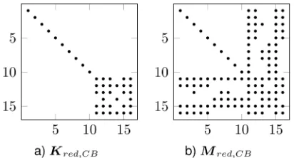
The sparsity pattern of the reduced stiffness

matrix Kred and reduced mass matrix Mred MN, of the

CBM (Fig. 3), the MNM (Fig. 5), the RM (Fig. 6) and the DCBM (Fig. 4), respectively, illustrate the differences of the assembled reduced structures. Both

the reduced stiffness matrix K_red and the reduced

mass matrix Mred applying the CBM and the DCBM,

respectively, have only diagonal entries for the subparts of each substructure. On the one hand the coupling between the substructures using the CBM is entirely achieved by the last rows and last columns in

the mass matrix M_{red CB,} (Fig. 3b) and the remaining

part is diagonal [2]. On the other hand the coupling

applying the DCBM is entirely achieved by the last rows and last columns in the stiffness matrix K_{red DCB,}

(Fig. 4a) and again the remaining part is diagonal [6].

The corresponding degrees of freedoms are either the

interface displacements ub or the interface forces λλ

but no direct coupling between the modal parameters of adjacent substructures occurs which ensures the sparse structure.

Fig. 3. Sparsity pattern of the reduced matrices applying the CBM using 5 normal modes per substructure

Fig. 4. Sparsity pattern of the reduced matrices applying the DCBM using 5 normal modes per substructure

In contrast the sparsity pattern of the reduced

Mred obtained by the MNM and the RM, respectively, show full matrices. The MNM gives indeed an entirely

diagonal reduced mass matrix Mred MN, (Fig. 5b) but

causes always a full coupling between all DOF of all substructures via the reduced stiffness matrix K_{red MN,}

(Fig. 5a). This makes the reusability of reduced models obtained by the MNM very inefficient and therefore nearly impossible from a practical point of view. The RM also causes a coupling between the

substructures via interface displacements ub in the

reduced stiffness matrix Kred R, (Fig. 6a) as well as in the reduced mass Mred R, (Fig. 6b).

Fig. 5. Sparsity pattern of the reduced matrices applying the MNM using 5 normal modes per substructure

Fig. 6. Sparsity pattern of the reduced matrices applying the RM using 5 normal modes per substructure

Moreover all DOF belonging to one reduced substructure are coupled with all other DOF of the same substructure which is why the reduced matrices of the RM are full for the substructure blocks and not diagonal. This result concerning the sparsity of the reduced matrices is outlined in Table 1 which shows

the number n of non-zero elements in the reduced

matrices K_red and M_red and the sum n_total of both

obtained by the different methods for this example. The reduced matrices of the CBM, the MNM and the DCBM contain a similar number of entries while the RM causes even for such a simple example a remarkable high number of entries. The number of entries of the MNM are comparable to the CBM and the DCBM but will increase dramatically if the

number of substructures is increased since Kred will

always be completely full.

Table 1. Number n of non-zero elements in the reduced matrices obtained by the different methods for the Benfield truss (5 normal modes per substructure)

CBM MNM RM DCBM

n in Kred 40 216 314 196

n in Mred 118 16 354 50

ntotal 158 232 668 246

3.2 Beam Frame

In [6] a three-dimensional frame made of steel beams

(Young‘s modulus 210 GPa, Poisson‘s ratio 0.3, and

density 7500 kgm3_{) schematically shown in Fig. 7 is}

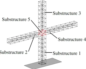
considered. Each cell in the frame has a height of 0.35 m and a width and depth of 0.5 m. All outer beams have a hollow circular cross-section with the outside and inside diameters 0.02 m and 0.018 m. The diagonal members inside the cells have a solid circular cross section with diameter 0.008 m. The frame is divided into 5 substructures and again the objective is

the approximation of the lowest eigenfrequencies ω

of the frame. Approximation of the eigenfrequencies of this system using the four presented methods with 4 normal modes per substructure (rigid body modes are not counted as free interface normal modes) is carried

out. The results presented in [6] for the DCBM were

obtained based erroneously on an incomplete set of free interface modes in the substructures using a simple Lanczos eigensolver: modes related to multiple frequencies were not determined by the simple Lanczos algorithm applied in that work.

Considering the geometry of the beam frame structure of the arms in Fig. 7, the symmetry of the substructures is identifiable resulting in multiple eigenfrequencies of the substructures. The simple Lanczos eigensolver (no blocks, no restarts) used in

[6] was not capable of determining multiple

eigenvalues reliably [11]. Hence, when the simple

Lanczos algorithm is used to determine the free modes of the substructure, modes that are multiple are missing and the representation of the lower spectrum is incomplete. Normal modes associated to the higher eigenfrequencies computed by the simple Lanczos eigensolver are used leading to poor approximation accuracy. Using the block Lanczos method and taking the lowest eigenfrequencies with associated subspaces of eigenvectors, the accuracy of the eigenfrequencies of the reduced global system obtained by the two reduction methods increases in the low frequency

range [11]. In this work we are using an eigensolver

capable of determining multiple eigenvalues for the comparison of the results obtained by the different

methods. Again the eigenfrequencies ω_red of the

reduced system applying the CBM, the MNM and the

DCBM as well as the eigenfrequencies ω_full of the

full (non-reduced) system are computed. The

eigenfrequency relative errors

ε_{rel j,} =ω_{red j,} −ω_{full j,} /ω_{full j,} comparing the eigenfrequencies of the non-reduced model with the

eigenfrequencies ω_red of the reduced system obtained

by the reduction methods are plotted in Fig. 8.

Nevertheless, as already observed in [6], this confirms

that the accuracy of the DCBM in the low frequency

range is two orders of magnitude better than the CBM. Comparing only the free interface methods, the RM performs slightly better than the DCBM. Both the RM and DCBM give a much better approximation accuracy than the MNM.

3.3 Two-dimensional solid

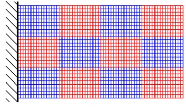
In order to emphasize the weak coupling between the substructure interfaces applying the DCBM, as described in section 2.2.3, the problem of a two

dimensional rectangle (density ρ, Young‘s modulus E,

Poisson‘s ratio ν = 0.3) decomposed in 12 substructures

as illustrated in Fig. 9 is considered. Each substructure

is discretized by 16×9 bilinear four-noded elements

(plane stress) and the structure is clamped on the left side in both directions. Again the objective is to

approximate the lowest eigenfrequencies ω of the

entire structure with the four different methods. Using 8 normal modes per substructure (not including potential rigid body modes) the relative errors

ε_{rel j,} =ω_{red j,} −ω_{full j,} /ω_{full j,} depicted in Fig. 10 are resulting.

Making use of such a large reduction basis the DCBM and the RM give excellent results in the low frequency range in comparison to the CBM and the MNM. Approximating the 20 lowest eigenfrequencies of the full structure, neither compatibility problems nor trouble with negative eigenfrequencies occur during the reduction process with the DCBM. Similar

graphs depicting the relative errors ε_rel as in Fig. 10

are obtained using different numbers of normal modes per substructure for the four methods.

When considering a very small reduction basis for the substructures (using only a small number of normal modes), non-physical negative eigenvalues of the reduced problem show up in the low frequency

Fig. 8. Relative error εrel j, of eigenfrequency j using 4 normal

modes per substructure for the approximation of the lowest eigenfrequencies of the entire beam frame

Fig. 9. Two dimensional solid problem (dimensionless width lx = 16, height ly = 9 decomposed in 12 substructures; each

substructure is discretized by 16×9 bilinear four-noded elements (plane stress) and the structure is clamped on the left side in both

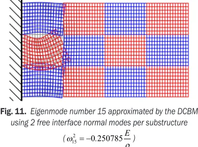
range. Using only 2 normal modes per substructure as reduction basis for this example negative values emerge among the 20 smallest absolute values of

eigensolutions ω2 _{applying the DCBM. In this case}

the first 14 of the lowest absolute values of ω2 _are

positive and the associated eigenmodes are approximating the true eigenvalues and eigenmodes of the full system accurately. But, as shown in Table 2,

the 15th _{eigenvalue is negative and the associated}

eigenmode depicted in Fig. 11 shows the non-physical behavior of this eigensolution.

Fig. 10. Relative errorεrel j, of eigenfrequency jusing 8 normal modes per substructure for the approximation of the lowest

eigenfrequencies of the entire structure

Table 2. Number j and associated eigenvalue ω_j2 of the two dimensional solid reduced with the DCBM

j ω_j ρ

E 2

1 0.000874

2 0.009729

⁞ ⁞

14 0.245011

15 -0.250785

16 0.261676

The eigenmodes corresponding to negative eigensolutions with higher absolute values show similar behavior. All these negative eigenvalues are related to the weak compatibility on the interfaces and not meaningful from a physical point of view. Consequently detecting and filtering out those negative eigenvalues is an additional step in the DCBM compared to the other methods based on primal assembly. This extra step is cheap and therefore does not increase the effort of the reduction process

using the DCBM compared to the other four methods keeping the DCBM very efficient.

Fig. 11. Eigenmode number 15 approximated by the DCBM using 2 free interface normal modes per substructure

(ω

ρ 15

2

0 250785

= − . E)

4 CONCLUSIONS

In this paper the general concepts of the Craig-Bampton method (CBM), the MacNeal method (MNM), the Rubin method (RM) and the dual Craig-Bampton method (DCBM) were briefly presented, compared and discussed using three examples. The DCBM is outperforming the CBM using the same number of normal modes per substructure as reduction basis with comparable computational effort and having similar sparsity pattern of the reduced matrices. Comparing the free interface methods, the RM performs slightly better than the DCBM but results in full matrices. Both the RM and DCBM give a much better approximation accuracy than the MNM while the MNM generated always full coupled reduced matrices.

Properties of the DCBM were outlined and an additional necessary step, namely filtering out the negative eigensolutions, during the reduction process was illustrated. Non-physical negative eigenvalues of the reduced dual assembled problem are intrinsic in the reduction process using the DCBM caused by the weak compatibility on the interfaces between the substructures. Filtering out these negative eigenvalues is the decisive factor for the excellent approximation quality of the DCBM. The numerical effort adding this additional step is negligible keeping the efficiency of this method.

5 REFERENCES

[2] Craig, R.R., Bampton, M.C. (1968). Coupling of substructures for dynamic analyses. AIAA Journal, vol. 6, no. 7, p. 1313-1319, DOI:10.2514/3.4741.

[3] MacNeal, R.H. (1971). A hybrid method of component mode synthesis. Computers & Structures, vol. 1, no. 4, p. 581-601,

DOI:10.1016/0045-7949(71)90031-9.

[4] Rubin, S. (1975). Improved component-mode representation for structural dynamic analysis. AIAA Journal, vol. 13, no. 8, p. 995-1006, DOI:10.2514/3.60497.

[5] Herting, D.N. (1985). A general purpose, multi-stage, component modal synthesis method. Finite Elements in Analysis and Design, vol. 1, no. 2, p. 153-164,

DOI:10.1016/0168-874X(85)90025-3.

[6] Rixen, D.J. (2004). A dual Craig-Bampton method for dynamic substructuring. Journal of Computational and Applied Mathematics, vol. 168, no. 1-2, p. 383-391, DOI:10.1016/j. cam.2003.12.014.

[7] Voormeeren, S.N., Van Der Valk, P.L.C., Rixen, D.J. (2011). Generalized methodology for assembly and reduction of

component models for dynamic substructuring. AIAA Journal, vol. 49, no. 5, p. 1010-1020, DOI:10.2514/1.J050724.

[8] Craig, R.R., Chang, C.J. (1977). On the use of attachment modes in substructure coupling for dynamic analysis. 18th Structural Dynamics and Materials Conference, San Diego, p. 89-99, DOI:10.2514/6.1977-405.

[9] Rixen, D.J. (2011). Interface Reduction in the Dual Craig-Bampton method based on dual interface modes. Linking Models and Experiments, vol. 2, Conference Proceedings of the Society for Experimental Mechanics Series, p. 311-328,

DOI:10.1007/978-1-4419-9305-2_22.

[10] Benfield, W.A., Hruda, R.F. (1971). Vibration analysis of structures by component mode substitution. AIAA Journal, vol. 9, no. 7, p. 1255-1261, DOI:10.2514/3.49936.