Interactive Learning and Generalization in Repeated Games: Theories, Models, and Experiments

U

NIVERSITY OF

T

RENTO

CIFREM

I

NTERDEPARTMENTAL

C

ENTRE FOR

R

ESEARCH

T

RAINING

IN

E

CONOMICS AND

M

ANAGEMENT

D

OCTORAL

S

CHOOL IN

E

CONOMICS AND

M

ANAGEMENT

I

NTERACTIVE

L

EARNING AND

G

ENERALIZATION IN

R

EPEATED

G

AMES

:

T

HEORIES

, M

ODELS

,

AND

E

XPERIMENTS

A DISSERTATION

SUBMITTED TO THE DOCTORAL SCHOOL OF ECONOMICS AND MANAGEMENT IN PARTIAL FULFILLMENT OF THE REQUIREMENTS

FOR THE DOCTORAL DEGREE (PH.D.)

IN ECONOMICS AND MANAGEMENT

Davide Marchiori

T

HESIS

S

UPERVISORS

Professor Massimo Warglien

Department of Business Economics and Management

& Advanced School of Economics

Ca’ Foscari University of Venice

Professor Alessandro Rossi

Department of Computer and Management Science

University of Trento, Italy

R

EFEREE

C

OMMITTEE

Professor Giovanna Devetag

Department of Law and Management

University of Perugia, Italy

Professor Ido Erev

Acknowledgements

Thanks to Judith Avrahami, Ido Erev, and Thorsten Chmura for having kindly provided me with their experimental datasets.

I am particularly grateful to Massimo Warglien, who supervised my work and funded my experiments. I am also indebted to Marco LiCalzi, Paolo Pellizzari, Paola Manzini, Marco Mariotti, Scott Page, John Miller, Shu-Heng Cheng, Werner Güth, and Armin Falk for their insightful and helpful suggestions and comments.

The organizational support of the CEEL laboratory staff (in particular of Marco Tecilla) and of its director Professor Luigi Mittone is also acknowledged.

C

ONTENTS

1. INTRODUCTION...1

1.1 OVERVIEW OF THE THESIS...2

1.1.1 Part One (Chapter 2)...2

1.1.2 Part Two (Chapter 3)...3

1.1.3 Part Three (Chapter 4) ...4

1.2 ON LEARNING IN REPEATED, COMPLETELY MIXED GAMES...5

1.2.1 Learning: Empirical Findings ...7

1.3 QUANTITATIVE MODELS OF LEARNING...9

1.3.1 Reinforcement Learning Models...9

1.3.2 Beliefs Learning Models ...13

1.4 REGRET AND CHOICE BEHAVIOR...16

1.4.1 Psychology of Regret ...17

1.4.2 Regret and Decision-Making Modeling...20

1.5 BEST RESPONSE AND BEHAVIORAL MODELS OF EQUILIBRIUM...26

1.6 SIMILARITY, CATEGORIZATION, AND GENERALIZATION...30

1.7 MODELING CATEGORIZATION AND GENERALIZATION WITH NEURAL NETWORKS 35 1.8 METHODOLOGICAL APPENDIX...40

2. PREDICTING HUMAN BEHAVIOR BY REGRET-DRIVEN NEURAL NETWORKS ...47

2.1 MODELS OF LEARNING...48

2.2 THE PB MODEL...48

2.3 METHODS...54

2.4 THE DATA...56

2.5 SIMULATION RESULTS: ACTUAL PAYOFFS...59

2.6 SIMULATION RESULTS: RESCALED PAYOFFS...64

2.7 CONCLUSIONS...67

2.8 APPENDIX A. SUPPORTING MATERIAL...70

2.9 APPENDIX B. THE DATASET DESCRIPTION...82

2.9.1 Suppes and Atkinson (1960) ...82

2.9.3 O’Neill (1987) ... 83

2.9.4 Rapoport and Boebel (1992) ... 83

2.9.5 Ochs (1995) ... 84

2.9.6 Rosenthal, Shachat, and Walker (2003)... 85

2.9.7 Avrahami, Güth and Kareev (2005)... 86

2.9.8 Erev, Roth, Slonim and Barron (2007) ... 88

2.9.9 Selten and Chmura (2008) ... 90

3. NET REWARD ATTRACTIONS EQUILIBRIUM FOR STRATEGIC FORM GAMES AND ITS EXPERIMENTAL TEST ... 97

3.1 INTRODUCTION... 98

3.2 THE NRA EQUILIBRIUM... 99

3.2.1 Theoretical Framework... 100

3.2.2 Parametric NRA ... 106

3.2.3 Convergence to NRA Equilibrium... 107

3.3 RELATED WORK... 109

3.4 MODEL COMPARISON METHODOLOGY... 111

3.5 THE DATA... 113

3.6 RESULTS... 115

3.6.1 First 50 Trials... 116

3.6.2 Last 50 Trials ... 117

3.6.3 All Trials... 119

3.7 SUMMARY AND CONCLUSIONS... 120

4. LEARNING IN MULTI-GAME EXPERIMENTS ... 133

4.1 ECONOMIC MODELS OF GENERALIZATION AND EMPIRICAL EVIDENCE... 134

4.2 THE GENERALIZING PB MODEL... 136

4.3 EXPERIMENTAL DESIGN... 137

4.4 EXPERIMENTAL RESULTS... 139

4.5 METHODS... 142

4.6 SIMULATION RESULTS... 143

4.7 WHAT DO SUBJECTS LEARN? ... 147

4.8 CONCLUSIONS AND FURTHER RESEARCH... 152

4.9 APPENDIX A. SUPPORTING MATERIALS AND TABLES... 155

5. OVERALL CONCLUSIONS AND FURTHER RESEARCH ...159

5.1 PART ONE (CHAPTER 2) ...160

5.2 PART TWO (CHAPTER 3) ...161

5.3 PART THREE (CHAPTER 4) ...164

5.4 FURTHER RESEARCH...165

C

HAPTER

1

1.

I

NTRODUCTION

The topic of my Ph.D. thesis spans different disciplines, as it is in the fields of behavioral game theory, experimental economics, and agent-based modeling. Specifically, my research addresses issues of learning in repeated games and

generalization i.e., how human beings generalize and apply their acquired strategic skills to new strategic situations, and it heavily relies on and makes use of the tools of computational social sciences.

This work provides further evidence that insights from psychology and neuroscience can be successfully used to design agent-based models that help improve understanding of human decision-making processes and that these models can far outperform (neoclassical) standard economic theory in describing and predicting human choice behavior.

The aim of my Ph.D. thesis is to advance understanding of human choice behavior in repeated strategic interactions. This is potentially important, since it would help explain empirical phenomena that cannot be accounted for by standard economic theory, such as overbidding in auctions and overtrading in financial markets (Selten, Abbink, and Cox, 2005). A further confirmation of the relevance of this topic comes from Erev and Haruvy (2005:359): “[it] is our conviction that some of the most promising directions for learning research lie in the investigation of “small” repeated decisions that are made with little information and little deliberation”, and “Though small decisions are of small consequence to the individual making them, they are potentially of tremendous importance to firms and society”. In economics, interactive strategic situations are commonly modeled as games, in which the gain (or payoff) of an agent (or player) depends upon its own choice and the choices of the other players. All throughout my thesis I devote my attention to a particular class of games i.e., the class of two-person 2x2, completely mixed1 _{games. This choice is coherent with an}

established paradigm of analysis in the behavioral and experimental economics fields, and is not only necessary to disentangle the effects of reciprocation and adaptation

processes (Erev and Roth, 1998), but also particularly interesting for reasons explained below.

This project is well divided into three, recognizably distinct parts (addressed in Chapters 2-4, respectively) that constitute a wider, unitary, and coherent research project on how past experience affects current behavior in interactive decision tasks, as well as the formal modeling of this behavioral process. Section 1 offers an overview of the main argument by providing a brief summary of each part. In Section 2, I illustrate the motivations for which the topic of learning in repeated games is important and, specifically, why repeated games with a unique equilibrium in mixed strategies are noteworthy. Section 3 reviews the most important models of learning proposed in the behavioral game theory and experimental economics literature. Section 4 provides a background for the role of regret in models and theories of choice behavior. Section 5 illustrates some of the most popular concepts of equilibrium, alternative to the theory proposed by Nash (1950) and based on very different assumptions. These stationary concepts can be grouped into two main classes: best-response and behavioral models. Section 6 introduces the concepts of similarity, categorization, and generalization, reviewing some of the most important contributions on these topics in the field of cognitive psychology. Section 7 provides a short introduction to neural networks and their important properties as models of information categorization and generalization. Finally, a section on methodological issues related to model comparison and selection criteria concludes.

1.1

Overview of the Thesis

1.1.1 Part One (Chapter 2)

This part of my thesis deals with interactive learning in repeated decision tasks. In a paper coauthored with Professor Massimo Warglien (Marchiori and Warglien, 2008), I propose a new model of learning, the Perceptron-based (PB) model, which embeds the basic principles of Learning Direction Theory (Selten and Stoecker, 1986) and translates them into a neural network model.

The basic assumption of the PB model is that learning is driven by an ex-post

directional change is proportional to a measure of regret i.e., how much they have missed by not making this move. This is coherent with recent neuroscience research on individual decision making, according to which regret affects learning, and both neuro-physiological and behavioral responses to the experience of regret are correlated to its magnitude (Coricelli et al., 2005 and Daw et al., 2006).

Further extending and improving the methodology adopted by Marchiori and Warglien (2008), I test the PB model on a set of 35 different datasets drawn from different experiments on games with unique equilibria in mixed strategies in which the participants received a complete description of the payoff matrix and of their opponents’ choices. In addition, I compare the performance of the PB model with those of other six popular models of learning in the behavioral game theory literature. As a result, the PB model outperforms in accuracy Nash equilibrium and all other models of learning, with the exception of a model (Normalized Fictitious Play proposed by Ert and Erev, 2007) similarly based on regret.

1.1.2 Part Two (Chapter 3)

In the second part of my thesis I propose and analyze the formal properties and the predictive power of a new concept of equilibrium I call Net Reward Attractions (NRA) Equilibrium.

The NRA Equilibrium is a stationary concept designed for strategic form games and is based on behavioral assumptions about human choice behavior, rather than on the principle of full rationality. It is assumed that, in equilibrium, agents are not expected utility maximizers, but that, for a player, the propensity of choosing an action is proportional to its corresponding expected net reward – net reward being defined as the difference between the actual payoff and the minimum obtainable one, given other players’ moves. I simply assume here that players are attracted by actions, and that this attraction can be quantified in terms of how much, on average, an action is perceived as better than the others. I propose also a parameterized version of NRA I call Parametric NRA (pNRA), obtained by introducing a parameter

€

λ>0, which tunes players’

sensitivity to expected net rewards.

complementary, although not equivalent (as I show in Chapter 3), to that based on regret. In Loomes and Sugden’s (1982) regret theory, these two complementary aspects are fused together in the Rejoice/Regret function (see Section 4.2 of Introduction), and I show in Chapters 2 and 3 of my thesis that these two components can be separately used to successfully design models of choice behavior.

The intuition at the basis of the NRA model, that relative rewards are what matters in determining choice behavior rather than absolute payoffs, is coherent with recent neuroeconomic research (Tremblay and Schultz, 1999; Tobler, Fiorillo, and Schultz, 2005; Daw et al., 2006).

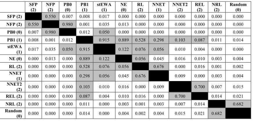
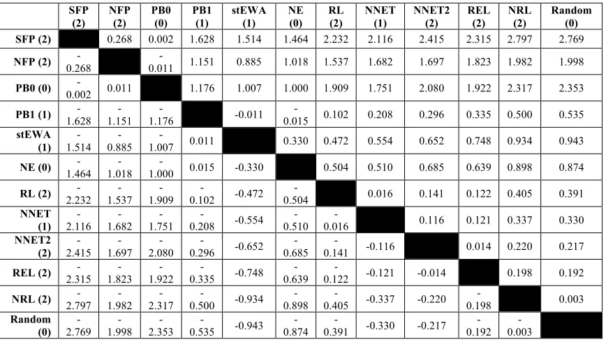
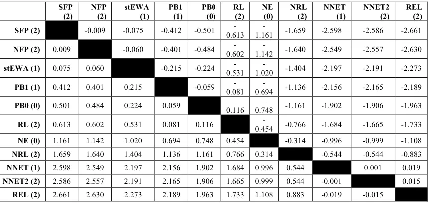
In part two of my thesis, I test the predictive accuracy of the NRA equilibrium on data from experiments on 26 repeated, completely mixed games run under full-feedback condition. In addition, I compare NRA’s predictive power with that of other five equilibrium concepts and eight models of learning, representing cutting-edge research on interactive decision making modeling. As a result, NRA turns out to be always among the best predictors of empirical data, performing significantly better than Nash equilibrium, self-tuning EWA, and reinforcement-based models.

1.1.3 Part Three (Chapter 4)

The third part of my thesis stands as a first attempt to investigate how do human subjects generalize their past experience when facing new strategic situations i.e., it addresses issues of conditional behavior and generalization.

With generalization I mean here the set of cognitive mechanisms and rules according to which subjects extract from past experience some general knowledge to deal with new, never encountered strategic situations. Issues of generalization and conditional behavior (different responses to different inputs) are relevant because most human interactive learning happens in contexts where tasks do not repeat themselves identically over time, contrary to the typical patterns of interaction that have been empirically studied until now. Generalizing from examples and learning of conditional behavior are natural features of human behavior.

I use my experimental data to test the predictive power of the Perceptron-Based (PB) model and compare it with that of other popular learning and equilibrium models of interactive choice behavior. It is worth noting here that conventional “attractions and stochastic choice rule” models of economic learning cannot capture such features of human behavior, since they are designed only for fitting and predicting data from situations in which subjects repeatedly play the same stage game. On the contrary, the architecture of the PB model accounts for this kind of dependence of behavior from the perception of changes in game payoffs.

As a result, the PB model outperforms in accuracy Nash equilibrium and all other models of learning as well. Further, I do not observe learning spillover effects in my experiments, which means that subjects are able to discriminate the different strategic situations and act accordingly. This fact might provide an explanation for why non-standard equilibrium models turn out to be the best predictors of my experimental data.

1.2

On Learning in Repeated, Completely Mixed Games

Despite their apparent simple structure, games with a unique mixed-strategy equilibrium (MSE) are worthy of particular consideration. Zero-sum games, which model a situation in which a player’s win corresponds to an opponent’s loss and vice-versa, are perhaps the most known and extreme example. In general, constant-sum games, of which zero-sum ones are a particular case, model situations of conflict, since players’ interests are opposed: in other words, players cannot help their opponents without being damaged. In this way, feelings such as fairness, reciprocity, and cooperation are almost completely excluded from this kind of interactions. Given their nature, these games faithfully portray situations of everyday life in which strict competitiveness is the most salient feature.

profile of common beliefs on the players’ moves and each player will choose an action that best responds to those beliefs; in this vein, a player chooses an action rather than a mixed strategy and an equilibrium is a steady state of players’ beliefs. Another interpretation is that proposed by Harsanyi (1973), who provides the proof that almost any MSE is the limit of pure strategy strict equilibria of opportunely chosen games whose payoffs are affected by random perturbations; therefore, players merely choose among their possible pure strategies, being the random fluctuations of the payoffs that lead players to use their pure strategies with the right frequencies.

From an experimental and behavioral point of view, however, this class of games represents a serious challenge for the predictive power of Nash equilibrium. Indeed, two strong – but behaviorally weak – assumptions stand at the core of the concept of Nash equilibrium. First, players are assumed to act in accordance with the theory of rational choice: they only care about the maximization of their own expected payoff, given their beliefs about the other players’ moves. Second, these beliefs are correct – in that sense players are said to be experienced.

In the realistic case of human, bounded-rational, and non-experienced players, it is not clear that an MSE can be learned and the question of how an equilibrium of play (if any) arises is still unanswered. There are at least four problems.

then, when two individuals from that population are randomly matched, it is impossible for them to guess the moves of their opponents, making this situation identical to that in which subjects choose randomly their pure strategies with probability 0.5.

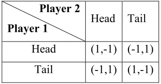
Player 2

Player 1 Head Tail Head (1,-1) (-1,1)

Tail (-1,1) (1,-1)

Figure 1. The matching pennies game, one of the most popular examples of zero-sum games.

1.2.1 Learning: Empirical Findings

Since the late 1950s, the experimental game theory literature on repeated games has provided significant departures from Nash equilibrium behavior (Erev and Roth, 1998) and especially data from experiments involving repeated games with unique MSE seem to contradict the predictions of standard game theory. In this specific context, indeed, Nash equilibrium not only fails to approximate laboratory observed behavior in the early rounds, but often it is also a poor predictor of the stable behavior emerging in the long run (Erev and Roth, 1998; Erev, Roth, Slonim, and Barron, 2007). As noted in Erev and Roth (1998:851) “in 5 of the 12 games equilibrium predicts badly: average choice probabilities, pooled over all rounds, are closer to random choices than to the equilibrium predictions”. The unsatisfactory performances of Nash equilibrium have led researchers to find alternative theories and models of learning to better explain and justify experimentally observed human behavior.

As a result, most of the models of learning proposed in the behavioral game theory literature outperform standard equilibrium theory in the tasks of fitting and predicting experimental data and these models attribute to other factors the role of drivers of choice behavior (Camerer, 2003; Erev and Roth, 1998; Erev, Bereby-Meyer, and Roth, 1999; Erev, Roth, Slonim, and Barron, 2002; Erev et al., 2007).

contributions by Walker and Wooders (2001), Chiappori, Levitt, and Groseclose (2002), Palacios-Huerta (2003), Palacios-Huerta and Volij (2006a, 2006b) show that the behavior of sport and chess professionals is “largely consistent with the minimax hypothesis” (Walker and Wooders, 2001:1521) and “remarkably consistent with equilibrium play in every respect” (Palacios-Huerta, 2003:395). One of the reasons of the discrepancy between on-field and lab-observed behaviors is that in the two cases players have different levels of experience with the situation they are facing. Indeed, as Walker and Wooders (2010) point out, “MSE is effective for explaining and predicting behavior in strategic situations at which the competitors are experts and less effective when the competitors are novices, as experimental subjects typically are”. Selten and Chmura (2008) propose another explanation: when a game is repeatedly played with random matching by two populations, subjects’ behavior can be quite different from that observed when the same game is played repeatedly by the same two individuals. In the latter case, playing hundreds of times against each other makes players focus on not being predictable by the other, which should reasonably push their behavior to minimax play. However, this explanation seems to be rather weak, since significant departures from MSE have been observed also in many experiments with fix-pairing protocol.

Could context be a further explanation for professionals’ behavior? Empirical evidence provides a negative answer to this question. Palacios-Huerta and Volij (2006a), indeed, observed the behavior of students and soccer professionals playing in laboratory settings a 2x2 game, formally identical to the typical strategic interactive situation of a penalty kick. The authors find that while professionals continue to play consistently with Nash theory, even in settings that entirely differ from those they are familiar with, college students perform quite poorly in terms of equilibrium play. This can be interpreted as evidence that professionals are able to transfer their strategic skills across different environments and that context has a negligible role in pushing subjects’ behavior to equilibrium play.

that individuals’ behavior is closer to that of college students than to professionals, and this justifies the need for experiments on repeated games.

1.3

Quantitative Models of Learning

Standard game theory does not provide a theory of learning and is limited to describing a steady state situation. On the contrary, experimentally observed behavior provides overwhelming evidence of the existence of a process – i.e. learning – after which past experience dramatically affects subjects’ current strategic choices (Camerer, 2003). Specifically, interactive learning differs from individual learning in that given N agents, each agent adapts to a strategic environment which is continuously modified by the concurrent learning of the other N-1 agents.

Learning models try to replicate artificially the process in which past experience affects agents’ current behavior; more specifically, they establish how the probabilities with which future actions will be chosen are affected by information about the outcomes produced by actions chosen in the past. In order to do this, quantitative theories assume that, for a player, all his possible actions are associated with numerical evaluations, called attractions or propensities (these two terms will be used interchangeably), which are mapped, according to opportune rules, into choice probabilities. Propensities can be interpreted as a measure of the propensity of a player to choose the actions they are associated with, while learning rules determine how these attractions are updated in response to past experience.

There is a wide variety of different approaches for modeling learning (for a comprehensive review of these models and theories see Camerer, 2003), but the most successful learning theories proposed so far are those of reinforcement learning, beliefs learning, hybrid models combining both (Ho, Camerer, and Chong, 2007) and, finally, theories which emphasize the role of post-decision regret as the driver of human behavior (Erev et al., 1999; Ert and Erev, 2007).

1.3.1 Reinforcement Learning Models

1. The Law of Effect: choices that have led to good outcomes in the past are more likely to be repeated in the future (Thorndike, 1898). This law implicitly assumes that choice behavior is probabilistic.

2. The power law of practice: learning curves tend to be steep initially, and then flatter (Blackburn, 1936).

3. Experimentation (or Generalization): not only the choices which were successful in the past are more likely to be employed in the future, but also similar choices will be employed more often (Erev and Roth, 1998).

4. Recency: recent experience plays a larger role than past experience in determining behavior (Erev and Roth, 1998).

Erev and Roth’s Reinforcement Learning (REL), the standard Reinforcement Learning (RL), and the Normalized Reinforcement Learning (NRL) models embed in their structure these four principles.

In reinforcement models, agents are assumed to have a very simple cognitive structure: they do not know anything about foregone or historical payoffs from strategies they did not choose, and occasionally experiment with the effects of similar choices. Here, only the actually played actions are reinforced. Typically, these models underestimate the empirical rate of learning, although correctly predicting its direction, being in the majority of the cases too slow to adapt to the observed dynamics. This seems to be due to the fact that in experiments in which subjects are provided with complete information about payoffs, they actually use that information in forming their strategies, while those models, by design, do not.

The REL Model

This model was first proposed in Erev et al. (1999) and further considered and developed in Erev et al. (2002). Here, I describe the REL model as reported in the latter contribution.

Attractions updating. The propensity of player i to play her k-th pure strategy at period t+1 is given by:

a_ij

(

t+1

)

=

a_ij

( )

t ⋅

[

N

( )

1 +C_ij

( )

t −1

]

+x

N

( )

1 +C_ij

( )

t if k = j

a_ij

( )

t otherwise,



 

where

€

C_ij

( )

t indicates the number of times that strategy j has been chosen in the first t

rounds, x is the obtained payoff, and

€

N

( )

1 a parameter of the model determining the weight of the initial attractions.

Stochastic choice rule. Player i’s attractions are mapped into choice probabilities by the following logistic rule:

€

p_ik

( )

t = exp

[

λ⋅aik

( )

t S t

( )

]

exp

[

λ⋅a_ij

( )

t S t

( )

]

j

∑

,

where

€

λ is a parameter tuning the sensitivity to payoff values, and

€

S t

( )

gives a measure of payoff variability.

Initial attractions. The value

€

S

( )

1 is defined as the expected absolute distance between the payoff from random choices and the expected payoff given random choices, denoted as

€

A

( )

1 . For period

€

t>1, the authors define:

€

S t

(

+1

)

= S t

( )

⋅

[

t+m⋅N

( )

1

]

+ A t

( )

−x t+m⋅N

( )

1 +1 ,

where x is the received payoff, m the number of player i’s pure strategies, and

€

A t

(

+1

)

is defined as:

€

S t

(

+1

)

= A t

( )

⋅

[

t+m⋅N

( )

1

]

+x t+m⋅N

( )

1 +1 .

The authors fix initial attractions as follows:

€

a_ij

( )

1 =A

( )

1 , for all i and j.

Thus, this model has two free parameters, namely

€

λ and

€

N

( )

1 .

The RL Model

This model has been proposed in Erev et al. (2007) and enriches the Basic Reinforcement model described in Erev and Roth (1999); the main difference between the two models is that in the latter, propensities are mapped into choice probability by simple normalization, while, in the former, this mapping is operated by a logit function.

Initial propensities. At time period

€

t=1, player i-th associates to the propensity of playing his pure strategy j, the value corresponding to the expected payoff from random choice (denoted by A

( )

1 ). Thus:

Attractions updating. At each time step, propensities are updated according to the following:

€

aij

(

t+1

)

=

1−w

(

)

⋅aij

( )

t +w⋅vik

( )

x if j=k

aij

( )

t otherwise,      where €

v_ij

( )

t is the realized payoff and w one of the two parameters of the model (sensitivity to foregone payoffs). The updating rule implies agents’ insensitivity to foregone payoffs.

Stochastic choice rule. Attractions at time

€

t are mapped into choice probabilities according to the rule:

€

p_ik

( )

t = exp

[

λ ⋅aik

( )

t

]

exp

[

λ ⋅a_ij

( )

t

]

j

∑

,

where

€

λ is a free parameter tuning sensitivity to payoffs. In the first period, the authors

suggest setting

€

recent_i =A

( )

1 .

The NRL Model

This model, described in Erev et al. (2007), is quite similar to REL and differs from RL in the fact that here payoff sensitivity is assumed to decrease with payoff variability.

Initial propensities. At time period

€

t=1, player i-th associates to the propensity of playing his pure strategy j, the value corresponding to the expected payoff from random choice (denoted by

€

A

( )

1 ). Thus:

€

a_ij

( )

1 =A

( )

1 , for all i and j.

Attractions updating. At each time step, propensities are updated according to the following:

€

aij

(

t+1

)

=

1−w

(

)

⋅a_ij

( )

t +w⋅v_ik

( )

x if j=k aij

( )

t otherwise,      where €

v_ij

( )

t is the realized payoff and w one of the two parameters of the model (sensitivity to foregone payoffs). The updating rule implies agents’ insensitivity to foregone payoffs.

Stochastic choice rule. Attractions at time

€

€

p_ik

( )

t = exp

[

λ ⋅aik

( )

t S t

( )

]

exp

[

λ ⋅a_ij

( )

t S t

( )

]

j

∑

,

where

€

S t

( )

gives a measure of payoff variability and

€

λ is a free parameter tuning

sensitivity to payoffs.

€

S t

(

+1

)

=

(

1−w

)

⋅S t

( )

+wmax

{

recent₁,recent₂

}

−v_ij

( )

t ,

where recenti is the most recent experienced payoff from action i. In the first period, the authors suggest setting

€

recenti =A

( )

1 ; in addition, the initial value

€

S

( )

1 is set equal to

€

λ. Similarly to the case of the NFP model, payoff sensitivity (the ratio

€

λ S t

( )

) is

assumed to decrease with payoff variability.

1.3.2 Beliefs Learning Models

The models of this class embed the principles of the beliefs learning theory and are generally much more sophisticated than reinforcement models. According to this theory, players are assumed to keep track of the history of all other players’ moves and form their beliefs about what other players will do based on this past information. The strategy that will be chosen is that which maximizes the expected payoff given the beliefs about other players’ actions.

Two very popular models derived from this theory are the fictitious play and

weighted fictitious play models. In the first, players keep track of the relative frequency with which other players have employed each strategy in the past, and then calculate the expected payoff given these beliefs and choose that with the highest expected value. While in this model all previous observations are equally salient, in the weighted fictitious play model distant experiences in the past are less salient than recent ones (recency effect).

The Normalized Fictitious Play (NFP), the Stochastic Fictitious Play (SFP), and the Self-Tuning Experience Weighted Attraction (stEWA) models belong to this class of models. The last model, however, would be better described as a hybrid model, blending the main features of reinforcement and fictitious play models; indeed, if parameters are constrained to specific values, it reduces to a simple version of the reinforcement model in which only chosen strategies are reinforced and if parameters are set in a different way, stEWA reduces exactly to weighted fictitious play.

choice probabilities; by construction, this function is extremely sensitive to how initial propensities are defined, and different approaches can dramatically affect the performances of these models.

The NFP Model

This model has been proposed by Ert and Erev (2007) and described in Erev et al. (2007).

Initial propensities. At time period

€

t=1, player i-th associates to the propensity of playing his pure strategy j the value corresponding to the expected payoff from random choice (denoted by

€

A

( )

1 ). Thus:

€

a_ij

( )

1 =A

( )

1 , for all i and j.

Attractions updating. At each time step, propensities are updated according to the following:

€

a_ij

(

t+1

)

=

(

1−w

)

⋅a_ij

( )

t +w⋅v_ij

( )

t , for all i and j, where

€

v_ij

( )

t is the expected payoff in the selected cell and w is one of the two parameters of the model (sensitivity to foregone payoffs).

Stochastic choice rule. Attractions at time

€

t are mapped into choice probabilities according to the rule:

€

p_ik

( )

t = exp

[

λ ⋅aik

( )

t S t

( )

]

exp

[

λ ⋅a_ij

( )

t S t

( )

]

j

∑

,

where

€

S t

( )

gives a measure of payoff variability and

€

λ is a free parameter tuning sensitivity to payoffs.

€

S t

(

+1

)

=

(

1−w

)

⋅S t

( )

+wmax

{

recent₁,recent₂

}

−v_ij

( )

t ,

where recenti is the last experienced payoff from action i. In the first period, the authors suggest setting

€

recent_i =A

( )

1 ; in addition, the initial value

€

S

( )

1 is set equal to

€

λ.

The SFP Model

Initial propensities. At time period

€

t=1, player i-th associates to the propensity of playing his pure strategy j the value corresponding to the expected payoff from random choice (denoted by

€

A

( )

1 ). Thus:

€

a_ij

( )

1 =A

( )

1 , for all i and j.

Attractions updating. At each time step, propensities are updated according to the following:

€

a_ij

(

t+1

)

=

(

1−w

)

⋅a_ij

( )

t +w⋅v_ij

( )

t , for all i and j, where

€

v_ij

( )

t is the expected payoff in the selected cell and w one of the two parameters of the model (sensitivity to foregone payoffs).

Stochastic choice rule. Attractions at time

€

t are mapped into choice probabilities according to the rule:

€

p_ik

( )

t = exp

[

λ ⋅aik

( )

t

]

exp

[

λ ⋅a_ij

( )

t

]

j

∑

,

where

€

λ is a free parameter tuning sensitivity to payoffs. In the first period, the authors suggest setting

€

recent_i =A

( )

1 .

The stEWA Model

Self-tuning Experience Weighted Attraction is a one-parameter model of learning in games proposed by by Ho, Camerer, and Chong (2007). It replaces part of the 5 parameters in an earlier model called EWA (Camerer and Ho, 1999) with functions of experience that operate a self-tuning over time.

Attractions updating. At time t, player i associates to his j-th pure strategy the attraction

€

a_ij

( )

t , given by:

€

a_ij

( )

t =φi

( )

t ⋅N t

(

−1

)

⋅aij

(

t−1

)

+

[

δij

( )

t +

(

1−δij

( )

t

)

⋅I s

(

ij,si

( )

t

)

]

⋅πi

(

sij,s−i

( )

t

)

N t

(

−1

)

⋅φ_i

( )

t +1 , where are parameters,

€

si

( )

t and

€

s−i

( )

t are the strategies played by player i and his opponents, respectively, and

€

π_i

(

s_ij,s_−i

( )

t

)

is the ex-post payoff deriving from playing strategy j. The function

€

I

( )

⋅ is defined as:

I x,

(

y

)

= 0 if x≠y 1 if x=y, 

while the functions

€

δ_ij

( )

t and

€

φi

( )

t are called, respectively, the attention function end the change detector function. The second depends primarily on the difference between the relative frequencies of chosen strategies in the most recent periods and the relative frequencies calculated on the entire series of actions. The attention function essentially tunes the importance that players associate to past payoffs (see Camerer, Ho and Chong, 2007 for details). Thus, attractions on time t depend on the attractions on time t-1 multiplied by an experience weight

€

N t

(

−1

)

, on received and foregone payoffs, and are pseudo normalized by the quantity

€

N t

( )

=N t

(

−1

)

⋅φi

( )

t +1 (

€

N

( )

0 =1).

Stochastic choice rule. Attractions are mapped into choice probabilities by the following equation:

€

p_ij

(

t+1

)

= exp

(

λ ⋅aij

( )

t

)

exp

(

λ ⋅a_ij

( )

t

)

j

∑

,

where

€

λ is the unique free parameter of the model.

Initial attractions. The authors do not provide a unique method to define initial attractions

€

a_ij

( )

0 and suggest at least four ways it might be done. In this specific case, I define initial attractions according to the method adopted for reinforcement models, which leads to first-period uniformly distributed choices.

1.4

Regret and Choice Behavior

The unsatisfactory performances of Nash equilibrium have led researchers to find alternative theories and models to better explain and justify experimentally observed interactive choice behavior.

will provide a short review of the principal contributions on regret proposed in the psychology literature, in order to more precisely define its meaning and nature.

1.4.1 Psychology of Regret

Behavioral economics, experimental economics, and psychology have devoted much attention to the effects of emotions on decision-making, and the literature on this topic is vast. If we consider all contributions on emotions and the role they play in shaping human choice behavior, regret has been the most studied. I will present some of the most important contributions, mainly from the field of psychology, investigating nature and properties of this counterfactual emotion.

Regret is generally defined as the emotion that a decision maker experiences whenever the outcome of his action is worse than the one he would have received, had he acted in a different way. A first distinction has to be done between regret and

disappointment; generally, these two emotions are reputed to be different and have been shown to produce different behaviors (Mellers, Schwartz, and Ritov, 1999; Zeelenberg, van Dijk, and Manstead, 1998). Disappointment arises whenever the received outcome is worse than the outcome one would have obtained in another state of the world. Therefore, the difference between these two negative emotions relies on the decision maker’s intervention (agency); for regret to occur, not only the actual outcome must be worse than foregone ones, but the decision maker must also consider himself as directly responsible for it by having chosen a specific course of action.

victims sometimes generate positive feeling by noting that they could have been more seriously injured or killed). As for the latter function, comparisons with better alternatives (called upward counterfactuals) can serve to develop patterns of future actions. Indeed, as Roese (1997) points out, counterfactual thinking is triggered when our choices have a negative effect i.e., in those situations in which corrective thinking is most important.

Two main factors have been shown to determine regret and its intensity: the first is the degree of availability of possible alternatives and, second, the active versus inactive attitude of the decision maker. Seta, Seta, McElroy, and Hatz’s (2008) experimental results show that the salience of counterfactuals is positively correlated with the intensity of experienced regret, coherently with Kahnemann and Miller’s (1986) norm theory. In addition, also mutability of events or states can affect the intensity of regret. The underlying idea is that if events can be changed in many ways, it is also true that some modifications are more natural than others as well as some attributes are easier to be changed than others. Kahnemann and Tversky (1982) show that exceptional features are more mutable than routine ones since the former explicitly provide alternative scenarios to the occurred state. Kahnemann and Miller (1986) further investigate the role of mutability and find that “an event is more likely to be undone by altering exceptional than routine aspects of the causal chain that led to it” (Kahnemann and Miller, 1986:143). From this point of view, when agents’ decisions involve active behavior, they are likely to be considered as exceptional features and generate regret (“If only I did not do that…”). On the opposite, when agents’ behavior is inertial (i.e., they do not act to change things), their choices are more naturally interpreted as routine features in the causal chain, and are less likely to generate regret.

that people not only anticipate emotions, but also take them into account when deciding (Larrick and Boles, 1995; Ritov, 1996; Bar-Hillel and Neter, 1996; Zeelenberg, Beattie, van der Pligt, and de Vries 1996; Zeelenberg and Beattie, 1997). In addition, Zeelenberg (1999) provides an explanation of how anticipated regret can lead to relatively risk seeking behavior, as previously experimentally shown by Larrick and Boles (1995) and Ritov (1996). Zeelenberg’s argument starts from the reasonable assumption that people are regret averse; regret is a negative and unpleasant emotion, and then people tend to make choices as to minimize it. Now, regret-minimizing choices can be either safe or risky; indeed, it can happen that risky options are those to which there corresponds the lowest level of regret. As a simple example, consider a situation in which an individual has to choose between two choices, one riskier than the other. Assume also that the riskier option will always be resolved, whereas the safer will only be resolved if chosen. Then, if the decision maker chooses the safer choice, he runs the risk of learning that the riskier option turned out to be better and then experiences regret.

Zeelenberg (1999) mentions five conditions, not yet experimentally tested, that might determine occurrence and intensity of anticipated counterfactual regret. First, regret is likely to be anticipated when available actions have similar degree of dominance. If an action is evidently dominant (for some particularly salient reason) with respect to the others, an agent will choose it without spending too much time thinking about its consequences, and he would not consider himself as particularly responsible for a possible bad or suboptimal outcome (of course, he would be

the decision making process might affect the level of anticipated regret, particularly high in situations in which people that are important to the agent expect him to carefully evaluate all alternatives or delay his choice.

As noted by Zeelenberg (1999), these five aspects deserve further empirical investigation, as their understanding would help design a psychological theory of regret aversion and determine its scope of applicability.

1.4.2 Regret and Decision-Making Modeling

As far as I know, Savage (1951 and 1954) was the first to formally introduce regret in a theory of decision-making. His theory of (statistical) decision-making applies to situations in which the utility of an individual depends upon his own choice and the occurrence of one of n mutually exclusive states of the world. It is assumed that agents know how their own utilities depend jointly upon their choices and the (unknown) state of the world that will occur, but they do not know the probabilities that are associated to each state of the world. Savage defined the loss associated to action a and state s as the difference between the best outcome over all possible actions (given state s) and the outcome from action a. Let us consider the following example proposed by Savage in which the decision maker has to decide whether or not to carry with him his umbrella. Two states of the world can take place: it might be rainy or shiny, and the decision maker does not know the probabilities of the two states. Suppose that the utility of the decision maker for each possible combination (action, state) is as reported in the following matrix:

State

Action Rain Shine

Carry 4 5

The corresponding matrix of losses will be then:

State

Action Rain Shine

Carry 0 5

Do not carry 14 0

Savage proposed as a decision rule the minimax principle, according to which the decision maker chooses the action that minimizes the maximum loss. This theory of choice allows for violations of the axiom of independence of irrelevant alternatives and is quite pessimistic, since the decision maker looks only at the worst possible state for each of his actions. For these reasons both normative and descriptive validity of the

important. This means that our utility is determined not only by the outcome from our choice (as assumed by von Neumann and Morgenstern’s theory), but also by outcomes corresponding to unchosen actions. As an example, if foregone outcomes are better than the obtained one, we would experience regret for not having chosen differently, with a consequent decrease in the utility level. On the opposite, if foregone outcomes are worse than the obtained one, we would then experience rejoicing for having made the best decision, and this would translate in an increase of utility. The concept of regret as illustrated above was not new in the early 1980s, but closely resembles the argument exposed in Savage (1951) in the ambit of the theory of statistical decision, with the difference that in regret theory probabilities associated to outcomes are known. Of course, the importance of what might have been can be assessed only in those cases in which all outcomes are known i.e., in those situations in which agents receive feedback about their actions. In the light of these considerations about utility, Loomes and Sugden (1982) and Bell (1982) proposed a model in which agents are supposed to maximize a modified utility function, which explicitly takes into account the role of regret. In a restricted version of this model formulated by Loomes and Sugden, the utility function is of the form:

€

m_ijk

=c_ij+R c

(

_ij−c_kj

)

, (1) where

€

m_ijk is the modified utility when action i has been chosen and the j-th state of the

world has occurred, with respect to the consequence of action k; similarly,

€

cij represents the choiceless utility, defined as the utility that the individual would derive from outcome x without having chosen it – as if it were exogenously assigned to the individual. This assumption about

€

cij is quite important because, in contrast with the concept of utility provided by von Neumann and Morgenstern, it provides a sort of utility measure free from any psychological implication. Psychological aspects are introduced in (1) through the real valued regret-rejoice function

€

R

( )

⋅ , which weights the difference between obtained and foregone utility. Obviously,

€

R

( )

⋅ is supposed to be

non-decreasing. In the limiting case in which

€

R c

( )

=0

€

∀c, (1) is equivalent to standard expected utility theory. In terms of (1), action

€

A_k is non-preferred to action

€

A_i if and only if:

p_j

[

c_ij−c_kj+R c

(

_ij−c_kj

)

−R c

(

_kj−c_ij

)

]

j=1

n

given that each of the n states of the world occurs with probability

€

p_j. As its authors suggested, equation (2) can be reformulated in terms of a function

€

Q

( )

⋅ such that

€

Q c

( )

=c+R c

( )

−R

( )

−c , obtaining:

€

p_j

[

Q c

(

_ij−c_kj

)

]

j=1

n

∑

≥0.

Now, individuals for which

€

Q

( )

⋅ is non-linear behave in such a way that might violate “consistently and knowingly the axioms of transitivity and equivalence without ever accepting, even after the most careful reflection, that they have made a mistake” (Loomes and Sugden, 1982:820). With this sentence, the authors challenge the assumption that choice behavior under uncertainty can be defined as rational if and only if it conforms to the axioms of von Neumann and Morgenstern’s expected utility theory. On the contrary, Loomes and Sugden propose the idea that agents whose choice behavior violates some of the axioms of expected utility theory is not necessarily

irrational, as it can still be described (as in the case of regret theory) in terms of a behavior that maximizes an opportunely defined (or, better, modified) utility function.

Loomes and Sugden (1987a) compare regret theory with the skew-symmetric bilinear utility theory (SSB) proposed by Fishburn (1982 and 1983). The approach followed by Fishburn is essentially axiomatic rather than psychologically based. The two theories are similar in that they both drop the transitivity axiom. However, Fishburn’s model cannot account for the isolation effect, as it is presented in terms of prospects rather than actions. On the other hand, if we consider the particular case of (statistically) independent prospects, regret theory and SSB are equivalent.

Loomes and Sugden (1987b) provide further empirical evidence of violations of the axioms of expected utility theory, supporting the hypothesis that individuals’ capacity to anticipate feelings of regret and rejoicing heavily affect choice behavior and confirming the need for a theory that takes explicitly into account this psychological aspect.

LDT is a qualitative theory of learning in repeated decision tasks and assumes that agents decide on the basis of the ex-post rationality principle: one looks at what might have been better in the previous instance of decision making and adjusts in this direction. The central point is that agents’ behavior is based on a qualitative and causal

representation of their environment. The feedback about actions chosen in the previous trial is a necessary condition for a qualitative and causal representation of the context in which the new decisions are taken. Such a representation of the world and feedback about previous choices are the two fundamental assumptions of LDT.

LDT is not a complete explanation of adaptive behavior and does not postulate that ex-post rationality is always sufficient in the explanation of the experimentally observed behavior. Sometimes other factors may influence the decisional process, leading to adjustments in the “wrong” direction. However, this theory assumes that ex-post rationality is more important than the other factors. These considerations lead to the following prediction: more frequently than randomly, changes in the parameters are in the direction suggested by ex-post rationality.

Due to its qualitative nature, LDT does not specify the probabilities with which changes will occur, and hence we cannot use it to make quantitative predictions. However, this theory provides important insights – largely supported by experimental data (Selten, Abbink, and Cox, 2001) – whose basic principles can be incorporated into other quantitative models.

Recently, also some game theorists have devoted their attention to regret. Contributions by Hart and Mas-Colell (2000 and 2003) and by Hart (2005) show the existence of some adaptive procedures of choice behavior, defined in discrete time and based on regret, that can be proved to converge to the set of correlated equilibria of a game (the notion of correlated equilibrium was first introduced by Aumann, 1974). The approach followed by the authors is almost exclusively theoretical, leaving no room for empirical tests of their models. The most important is the regret matching procedure introduced by Hart and Mas-Colell (2000) and defined by the following, simple rule:

“Switch next period to a different action with a probability that is proportional

The mathematical formulation of the rule above is as follows. Consider player i at time

€

T+1. The average obtained payoff over the first T periods is:

€

U= 1

T u i st

( )

t=1 T

∑

,

and denote with

€

j=sT

i _{the action chosen by player i at time T. For each available} alternative action

€

k≠ j, consider the average payoff that i would have obtained had he always played k instead of j in all previous trials:

€

V k

( )

= 1 T _t=1νt

T

∑

where

€

ν_t =

ui _k,s t

−i

(

)

ifs_ti

= j

ui s_ti,s_t−i

(

)

ifs_ti≠ j.

  

 

The regret associated to action k is then defined as:

€

R k

( )

=V k

( )

−U,

if the difference is positive and zero otherwise. According to regret matching, the probability

€

pT+1

( )

k with which action k is played at time

€

T+1 is proportional to

€

R k

( )

according to the following:

€

p_T+1

( )

k =

c⋅R k

( )

ifk≠ j

1− c⋅R k

( )

ifk≠ j,

k≠j

∑

    

where c is an opportune positive constant. Therefore, if at time

€

T+1, before choosing his action, player i has no regret (i.e., all

€

R k

( )

=0 for all

€

k≠ j), then he will play action

j for sure. If instead there are some actions

€

k for which

€

R k

( )

is positive, then the probability for player i to choose those actions will be different than zero and proportional to their corresponding regret.

The unconditional regret matching model (Hart, 2005) is obtained by slightly changing function

€

V k

( )

and replacing it with the following:

€

˜ V k

( )

= 1

T u

i

k,st

−i

(

)

t=1

T

∑

.

In this case

€

The most important results proved by Hart and Mas-Colell (2003) is that if all players play regret matching strategies, then the joint distribution of play converges to the set of correlated equilibria of the stage game. This result, known as the Regret Matching Theorem, is important as it shows that behavior of bounded rational agents can nonetheless converge to a rational outcome i.e., a correlated equilibrium. This result must then be seen as an effort to reconcile bounded rationality and rational behavior.

1.5

Best Response and Behavioral Models of Equilibrium

In spite of what reported at the beginning of Section 3, a stream of economic literature on non-standard equilibrium models has shown that also stationary concepts based on psychological considerations about human behavior are good predictors of data from experiments on auctions and repeated, completely mixed games (Selten, Abbink, and Cox, 2005; Ockenfels and Selten, 2005; Avrahami, Güth, and Kareev, 2005; Neugebauer and Selten, 2006; Selten and Chmura, 2008). In particular, I am referring to the Impulse Balance Equilibrium (IBE) model proposed by Ockenfels and Selten (2005). This stationary concept incorporates the principles of Learning Direction Theory (see previous section) in a quantitative theory. Specifically, its authors define

(described in Selten and Chmura, 2008, but previously formulated by Selten), agents are supposed to choose optimally with respect to the information from n samples of equal size (one for each available action), and from a sample of seven observations of the strategies played by their opponents, respectively. In both cases, the size of the sample can be interpreted as the unique free parameter of the two models. The concept of Quantal Response (QRE) equilibrium proposed by (McKelvey and Palfrey, 1995) can be considered as a generalization of the equilibrium model proposed by Nash (1950). It is based on the idea that players give quantal best responses to the behavior of the others i.e., players make mistakes and assume other players to do so as well; players are still supposed to be maximizers, departing from Nash’s theory in that perfectly rational expectations are replaced with noisy, imperfect ones. Assuming a particular distribution of errors, along the theoretical framework proposed by McFadden (1976), McKelvey and Palfrey designed the Logit Equilibrium, which converges to Nash equilibrium as the free parameter of the logistic quantal response function tends to infinite.

Selten and Chmura (2008) show that the free parameters IBE model is the best predictor of the data from experiments on twelve 2x2 repeated, completely mixed games, if compared with the other stationary concepts mentioned in this Section. However, the authors raise two important, yet unanswered, questions: first, it is not clear why in some games equilibrium models with so different theoretical foundations provide equivalently accurate predictions; second, they do not test models on more general patterns of strategic interaction (e.g., games with more than two players and more than two actions available to each player).

I provide here a short description of each model of equilibrium in the particular context of two-person 2x2 games with a unique equilibrium in mixed strategies. A detailed description and a comparative analysis of these models is reported in Selten and Chmura (2008).

Player 2

Player 1 L R

U

€

aL+cL;bU

(

)

€

aR;bU+dU

(

)

D

€

aL;bD+dD

(

)

€

aR +cR;bD

(

)

where the constants

€

c_L,

€

c_R,

€

d_U, and

€

d_D are strictly bigger than zero. Let us assume that Player 1 will choose action U with probability p and that Player 2 will choose action L with probability q.

Quantal Response Equilibrium (QRE)

Quantal Response Equilibrium was first introduced by McKelvey and Palfrey (1995). Equilibrium probabilities are determined as follows:

€

p= e

λEU( )q

eλEU( )q

+eλED( )q and

€

q= e

λEL( )p

eλEL( )p

+eλER( )p ,

where

€

λ ≥0 is the unique free parameter of the model.

Action-Sampling Equilibrium (7-sampling)

Proposed by Reinhard Selten, this stationary concept assumes that players sample 7 actions made by their opponents and best respond based to that sample. Formally, choice probabilities are defined as follows:

€

p= 7 k





 



qk

(

1−q

)

7−kαU

( )

k k=0

7

∑

and

€

q= 7 m       m=0

7

∑

(

1−p

)

mp7−m

αL

( )

m , where

€

αU

( )

k is the probability with which Player 1 will choose U given k Ls in the

sample by his opponent, and

€

αL

( )

m the probability with which Player 2 will choose L given m Us in the sample. Those are defined as:

€

α_U

( )

k =

1 if k 7>

c_R c_L+c_R 1

2 if k 7=

c_R c_L +c_R 0 otherwise          and €

α_L

( )

m =

1 if m 7 >

d_U d_U+d_D

1 2 if

m 7 =

d_U d_U +d_D

Payoff-Sampling Equilibrium

This parametric stationary concept was introduced by Osborne and Rubinstein (1998). According to it, players are assumed to play each of their available actions for n (the parameter of the model) times, record their opponents’ moves, and best respond to those samples. In the case of 2x2 games, suppose that

€

k_U and

€

k_D are the number of Ls in the two samples of Player 1, whereas

€

m_L and

€

m_R are the number of Us in the two samples of Player 2. Then, the probabilities with which Player 1 chooses U and Player 2 chooses R are, respectively:

€

β

(

k_U,k_D

)

=

1 if k_U

(

a_L+c_L

)

+

(

n−k_U

)

a_R >k_Da_L +

(

n−k_D

)

(

a_R +c_R

)

1

2 if kU

(

aL +cL

)

+

(

n−kU

)

aR =kDaL +

(

n−kD

)

(

aR +cR

)

0 otherwise

       , and € €

γ

(

m_L,m_R

)

=

1 if m_Lb_U+

(

n−m_L

)

(

b_D+d_D

)

>m_R

(

b_U+d_U

)

+

(

n−m_R

)

b_D

1

2 if mLbU+

(

n−mL

)

(

bD+dD

)

=mR

(

bU+dU

)

+

(

n−mR

)

bD 0 otherwise

       ,

Choice probabilities are defined as the expectation of the

€

β and

€

γ functions:

€

p= n

k_U       n k_D       kD=0

n

∑

qkU+kD

(

_1−q

)

2n−kU−kD_{β k}

U,kD

(

)

kU=0

n

∑

€

q= n

m_L 

  

  n_m

R       mR=0

n

∑

(

1−p

)

mL+mR

p2n−mL−mR_{γ m}

L,mR

(

)

mL=0

n

∑

.

Impulse Balance Equilibrium (IBE)

This concept of equilibrium is based on the qualitative Learning Direction Theory (LDT), proposed by Selten and Buchta (1999). According to Impulse Balance Equilibrium (Selten, Abbink, and Cox, 2005; Ockenfels and Selten, 2005), equilibrium probabilities are obtained as follows:

€

p= qcL

*

qc_L*

+

(

1−q

)

c_R* and

€

q=

(

1−p

)

dD *

pd_U*

+

(

1−p

)

d_D* , Constants € cL *_, € cR *_, € dU

*_{, and}

€

dD

* _{are the payoff differences the transformed game}

1.6

Similarity, Categorization, and Generalization

Issues of similarity, categorization, and generalization have been deeply and systematically investigated in the field of cognitive psychology in the 1970s and 1980s (Holland, Holyoak, Nisbett, and Thagard, 1986). These concepts are intimately linked, as similarity judgments about objects or events affect the way in which they are categorized (but the other way around holds true, too), and our responses, as human beings, depend upon past learning and categorization. In this vein, that of categorization can be considered as one of the most fundamental functions of all living creatures.

Categorization takes place whenever two or more stimuli are treated equivalently and this can happen in many di