R E S E A R C H A R T I C L E
Open Access
Impacts of cloud microphysics on trade
wind cumulus: which cloud microphysics
processes contribute to the diversity in a
large eddy simulation?
Yousuke Sato
*, Seiya Nishizawa, Hisashi Yashiro, Yoshiaki Miyamoto, Yoshiyuki Kajikawa and Hirofumi Tomita
Abstract
This study investigated the impact of several cloud microphysical schemes on the trade wind cumulus in the large eddy simulation model. To highlight the differences due to the cloud microphysical component, we developed a fully compressible large eddy simulation model, which excluded the implicit scheme and approximations as much as possible. The three microphysical schemes, the one-moment bulk, two-moment bulk, and spectral bin schemes were used for sensitivity experiments in which the other components were fixed. Our new large eddy simulation model using a spectral bin scheme successfully reproduced trade wind cumuli, and reliable model performance was confirmed. Results of the sensitivity experiments indicated that precipitation simulated by the one-moment bulk scheme started earlier, and its total amount was larger than that of the other models. By contrast, precipitation simulated by the two-moment scheme started late, and its total amount was small. These results support those of a previous study. The analyses revealed that the expression of two processes, (1) the generation of cloud particles and (2) the conversion from small droplets to raindrops, were crucial to the results. The fast conversion from cloud to rain and the large amount of newly generated cloud particles at the cloud base led to evaporative cooling and subsequent stabilization in the sub-cloud layer. The latent heat released at higher layers by the condensation of cloud particles resulted in the development of the boundary layer top height.
Keywords:Large eddy simulation; Shallow clouds
Background
The effect of clouds is one of the most uncertain factors in climate projection and numerical weather prediction. Shallow clouds (e.g., stratus, stratocumulus, shallow cu-mulus) play particularly important roles in the energy budget of the earth through radiation process because they cover a broad area of the earth (e.g., Randall et al. 1984). The 5th Intergovernmental Panel on Climate Change (IPCC) report suggested that the uncertainties with regards to shallow clouds should be reduced for re-liable assessments (IPCC AR5, Stocker et al. 2013).
In global scale models (e.g., general circulation model (GCM)) and regional models with coarse grid spacing, shallow clouds are usually expressed by parameterizations
(e.g., Tiedtke 1993; Considine et al. 1997; Kain 2004), but these parameterizations have not been able to effectively simulate the shallow cloud cover observed from satellites (e.g., Chepfer et al. 2008; Naud et al. 2010).
To improve the expression of shallow cloud, the re-sults of large eddy simulation (LES) models have been utilized. For example, Bretherton and Park (2009) used the results of an LES model to develop a new moist tur-bulent parameterization. Suzuki et al. (2004) and Posselt and Lohmann (2008) introduced an autoconversion parameterization that was typically used in an LES model (Khairoutdinov and Kogan 2000) into a global scale model. Many studies using LES models have been conducted to determine the characteristics of shallow cloud and improve large-scale modeling (e.g., Wang and Feingold 2009; Xue et al. 2008, Savic-Jovcic and Stevens 2008, Yamaguchi and Randall 2012). However, the
* Correspondence:[email protected]
RIKEN Advanced Institute for Computational Science, 7-1-26 Minatojima-Minami-machi, Chuo-ku, Kobe, Hyogo 650-0047, Japan
results of LES models are diverse, as indicated by several LES model intercomparison studies targeting shallow cloud (e.g., Stevens et al. 2005; Ackerman et al. 2009; van Zanten et al. 2011; Siebesma et al. 2003). It has been suggested that the difference in the microphysical schemes used in LES models is one of the reasons for the diversity in the results (Ackerman et al. 2009; van Zanten et al. 2011). However, it is difficult to investigate the exact effect of the different cloud microphysical schemes (i.e., the ef-fect on the results that comes from changing the cloud microphysical scheme while keeping all other components fixed), because each LES model uses a different scheme, not only in cloud microphysics but also many other com-ponents (e.g., governing equation, turbulent scheme, ad-vection scheme, and others). Thus, it is also difficult to determine which microphysical processes contribute most to the diversity of the LES results. Sensitivity experiments, which change only the cloud microphysical scheme, are required to better understand the exact effects of the cloud microphysical scheme.
The kinematic driver (KiD) model developed by Shipway and Hill (2012) enables us to conduct sensitivity simula-tions by changing only the cloud microphysics. Using KiD, we can consider the exact effects of the differences in cloud microphysical schemes. However, KiD ignores feedbacks to the atmosphere, even though the feed-backs of microphysics can affect the microphysical properties of shallow clouds and the turbulent struc-ture of the boundary layer (e.g., Stevens et al. 1998; Wang et al. 2010). It is necessary to consider the feed-back of microphysical processes on the dynamics when determining which process causes the diversity in the results of LES models. We should use the model that excludes approximation and implicit schemes as much as possible, because these features also affect the cloud microphysical properties simulated by the model.
This study developed a model that satisfies these re-quirements. Using the model, we attempted to repro-duce the diversity in the results of the LES model used in van Zanten et al. (2011) and to determine impact of the various cloud microphysical schemes. Three types of cloud microphysical schemes (one-moment bulk, two-moment bulk, and spectral bin schemes) were considered in this study, because these three schemes have been used in previous intercomparison studies.
Of the several types of shallow cloud, we focused on trade wind cumulus because their variability in the re-sults of LES models was larger than that of other types of shallow clouds. For example, the variability of surface precipitation in an intercomparison of trade wind cumu-lus (van Zanten et al. 2011) was larger than that in an intercomparison of stratocumulus (Ackerman et al. 2009). van Zanten et al. (2011) proposed that one of the reasons for the diversity in the microphysical properties
of trade wind cumuli was the different cloud microphys-ical models. They interpreted that a simple (one-moment bulk) microphysical scheme produced large amounts of precipitation (i.e., Table 3 of van Zanten et al. (2011)) and liquid water simulated by one-moment bulk schemes tended to be distributed in the lower layer. By contrast, the liquid water was located in the higher layer, and the precipitation flux was small in most of the two-moment schemes (i.e., Figure 6a of van Zanten et al. (2011)). In this study, we confirmed the validity of their interpretation through a simulation using our new fully compressible LES model and determined the main processes contribut-ing to the diversity in the results of LES model intercom-parison studies.
Methods
Experimental setup, dynamic framework, turbulence model, and external forcing
This section describes the common parts of the model with its experimental setup (i.e., the dynamic framework, turbulence model, and external forcing). The different parts of the microphysical schemes are highlighted in the subsequent section.
The dynamic model used in this study is an LES model that is included in the Scalable Computing for Advanced Library and Environment library (SCALE). Henceforth, we call this LES model SCALE-LES. The details of SCALE-LES are found at http://scale.aics.ri-ken.jp/.
A fully compressible system is adopted for the govern-ing equation of SCALE-LES. The prognostic variables are the three-dimensional momentum (ρu, ρv, ρw), total density (ρ), mass-weighted potential temperature (ρθ), and mass concentration of tracers (ρqs), where qs in-cludes specific humidity, ratio of mass, and number con-centration ratio of hydrometeors to total mass. Explicit time integration is used in all directions. Furthermore, the fourth-order central difference scheme is adopted for spatial discretization to avoid the numerically impli-cit diffusion that would be induced by odd-ordered dif-ference schemes. The three-step Runge–Kutta scheme is adopted. To retain stability of the model, fourth-order superviscosity/diffusion is applied for all prognostic vari-ables. Using SCALE-LES, developed as described above, we exclude the effects of approximation in the governing equation system and implicit diffusion as far as possible, enabling a consideration of the effects of the target com-ponent (i.e., cloud microphysics in this study).
The experimental setup is almost the same as that of the previous Global Energy and Water Exchange pro-ject (GEWEX) Cloud System Study (GCSS) intercom-parison of Rain in Cumulus over the Ocean (RICO) (van Zanten et al. 2011). The calculation domain covers 12.8 × 12.8 km2 horizontally with a double periodic boundary condition and 4.0 km vertically. The horizontal and vertical grid intervals are 100 and 40 m, respectively. Rayleigh damping is applied for three-dimensional mo-mentum over the upper atmosphere of z> 3.5 km. The strength of the numerical diffusion is set as 1.25 × 10⁵m4s−1, which is determined by the sensitivity experi-ment (the results of the sensitivity experiexperi-ment are shown in Appendix 1 of this paper). The simulations are con-ducted for 24 h with time steps (Δt) of 0.05, 0.15, and 0.5 s for dynamics, cloud microphysics, and other physics. TheΔtfor cloud microphysics is determined as the largest time step to avoid artificial noise, and the ratio of Δt for dynamics toΔtfor other physics is set to 10 based on the sensitivity experiments (see Appendix 2 of this paper for details of the sensitivity experiment).
The external forcing of the radiation, the surface flux, and the large-scale horizontal advection are applied in the same way as in van Zanten et al. (2011). The forcing of the large-scale subsidence is applied for all prognostic vari-ables including density, except for u and v. In nature, large-scale subsidence generates a divergence of total density, which makes the air mass flow out from the do-main. However, it cannot flow out in the compressible model using the configuration of van Zanten et al. (2011) due to the periodicity in the lateral boundary condition. Although this problem can be ignored in the anelastic and Boussinesq systems due to the fixed density, it is necessary to consider this problem in the compressible system. Although no description is available for this problem in van Zanten et al. (2011), the density of each layer should be reduced according to the diver-gence. The density reduction rate and the equation system with large-scale forcing are given below.
Large-scale subsidence (wLS) was given by van Zanten et al. (2011) as:
wLS¼
−0:005
2260z ðz<2260 mÞ
−0:005 ðz≥2260 mÞ 8
< :
where z is the height. Instead of this formulation, we give the subsidence formulated directly to vertical mo-mentum as:
ρwLS¼
−0:005
2260z ðz<2260 mÞ
−0:005 ðz≥2260 mÞ 8
< :
Consequently, the density reduction rate (D) is given as:
D≡∂ðρwLSÞ
∂z ¼
−0:005
2260 ðz<2260mÞ 0 ðz≥2260mÞ 8
< :
The continuous equation modified with the subsidence term is given by
∂ρ ∂tþ
∂ð Þρu
∂x þ
∂ð Þρv
∂y þ
∂ðρðwþwLSÞÞ
∂z ¼D ð1Þ
The density reduction derived from the divergence by the large-scale subsidence is added in the right-hand side (rhs) of Eq. (1). Note that this equation is identical to the equation without large-scale subsidence. The Lagrangian conservation equation of the scalar quantities (ϕ) is given as:
ρ∂∂ϕt þρu∂∂ϕxþρv∂∂ϕyþρðwþwLSÞ∂∂ϕz ¼0 ð2Þ
The prognostic variable of SCALE-LES is a mass-weighted value, and the equation of mass-mass-weighted values is derived from Eqs. (1) and (2) as:
∂ð Þρϕ
∂t þ
∂ðρuϕÞ
∂x þ
∂ðρvϕÞ
∂y þ
∂ðρðwþwLSÞϕÞ
∂z ¼Dϕ
ð3Þ
As shown in the rhs of Eq. (3), the scalar quantities (ϕ) flow out from each layer of the system by subsid-ence. The equation for the vertical momentum is modi-fied, as is that of the scalar quantities. The vertical flux ρwLSϕ at the top boundary can be determined so that such additional convergence of the flux is canceled with Dϕat the top layer.
Three microphysical schemes
To reproduce the diversity in the results of the RICO study, three types of cloud microphysical scheme are used for this study: the one-moment bulk microphysical scheme (Tomita 2008), the two-moment bulk scheme (Seiki and Nakajima 2014), and the spectral bin micro-physical scheme (Suzuki et al. 2010). The one-moment bulk scheme and the two-moment bulk scheme are based on Berry (1968) and Seifert and Beheng (2001), re-spectively. Both of the original bulk schemes were used in the RICO study.
from the one-moment bulk scheme in the assumption about the type of size distribution function and in the process of its determination. The two-moment bulk scheme assumes the generalized gamma distribution as the size distribution function, and the size distribution itself is determined not only by the mass concentration but also by the number concentration. In this sense, the two-moment bulk scheme is more sophisticated than the one-moment bulk scheme. The spectral bin scheme is an intrinsically sophisticated method compared with the others. It explicitly predicts the size distribution. To compensate for the detailed expression of size distribu-tion, the spectral bin scheme requires about four- to fivefold larger number of prognostic variables compared with the other two schemes.
Although the three microphysical schemes treat both warm and ice phase cloud, the ice phase was not calcu-lated because the temperature at the model top is greater than 273.15 K. In this case, the categorization of hydrometeors for each scheme is as follows. The one-moment and two-moment bulk schemes address two types of hydrometeors: cloud droplet and raindrop for warm rain process. The spectral bin scheme addresses only a type of water drop, which covers the particle size of both cloud droplets and raindrops. For the spectral bin scheme, the radius of newly generated cloud particles by nucleation is set to 3 μm (Suzuki et al. 2006). The size distribution of hydrometeors is discre-tized to 33 bins; its configuration has been established by several previous studies (e.g., Khain and Sednev 1996; Iguchi et al. 2008). The center of mass ofith bin (mi) is set by using the i-1-th bin (mi-1) as mi= 1.874 mi-1. m1 is the mass of cloud particles whose radius is
3μm.
All three schemes consider the generation of cloud droplets, condensation, evaporation, and sedimentation of cloud hydrometeors. Although the two-moment bulk scheme also considers the breakup of cloud droplets, this difference is minor based on sensitivity experiments examining the breakup process (figure not shown). Sedi-mentation is calculated by the first-order upwind scheme for all three schemes.
Since the generation of new cloud droplets is one of the critical processes in this experiment, the difference in this process among the schemes should be noted. The mass of newly generated cloud droplets is calcu-lated by saturation adjustment in the one-moment bulk scheme, which was also used in some one-moment bulk schemes in the RICO study. By contrast, it is calculated by the nucleation schemes in the two-moment bulk and spectral bin schemes. The number concentration of the cloud droplets (Nc,nucl) generated by the nucleation process is calculated as follows (e.g., Pruppacher and Klett 1997):
Nc;nucl¼ N0Swk; ð4Þ
where Sw is supersaturation over water. The constants N0 and k are set as N0= 100 × 106 m−3 and k= 0.462.
This scheme was also used in several models used in the RICO study. The growth of cloud droplets into rain-drops is another key issue for this experiment, as well as the underlying creation process. In the bulk scheme, this is expressed as autoconversion and accretion. To investi-gate the strength of the impact of the autoconversion and accretion processes, we conducted the same simula-tion with autoconversion and accresimula-tion ratios that were twice as large (0.067-fold smaller) as the two-moment (one-moment) scheme. The autoconversion rate (Pauto)
in the one-moment bulk scheme is calculated as in Tomita (2008), which was based on Berry (1968):
Pauto¼ 1
ρ 16:7ðρqcÞ 2
5þ3:610
−5N
c;T08
Ddρqc
kg kg‐1s‐1
;
ð5Þ
where Dd= 0.1456−5.964 × 10⁻² log (Nc,T08/2000), qc is
the cloud water mixing ratio, and Nc,T08 is the number
concentration of cloud droplets. In Tomita (2008),
Nc,T08 was set as 50 cm−3, but in this study, Nc,T08 was
set as 70 cm−3 based on the experimental setup in the RICO study (van Zanten et al. 2011). Another autocon-version scheme from Khairoutdinov and Kogan (2000) was implemented into the one-moment bulk scheme be-cause it had performed better than the scheme of Berry (1968) in a GCM (Suzuki et al. 2004). The scheme was also adopted in some models used in the RICO study.
Pauto in the Khairoutdinov and Kogan (2000) scheme is
calculated as:
Pauto¼1350q2:47c N−c;T081:79 kgkg‐1s‐1
ð6Þ
Using the schemes shown above, we attempted to reproduce the diversity of the LES results in the RICO study.
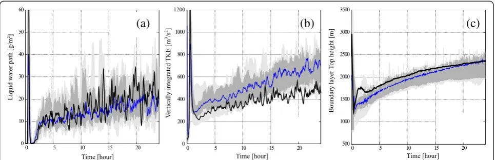
Results and discussion Basic performance of SCALE-LES
for several quantities. This indicates that our model could reproduce the shallow cumulus simulated by the LES models used in the previous study.
As well as the physical performance, the computa-tional performance and the scalability of SCALE were investigated. The elapsed time for a time step (Δt) and the performance efficiency are shown in Table 1. The elapsed time and performance of SCALE-LES do not change when it is used with a large number of Message Passing Interface (MPI) processes (e.g., over 10,000 MPI processes). This indicates that SCALE-LES has excellent scalability and a reasonable performance in massive par-allel computing.
Impacts of cloud microphysical scheme on simulation results
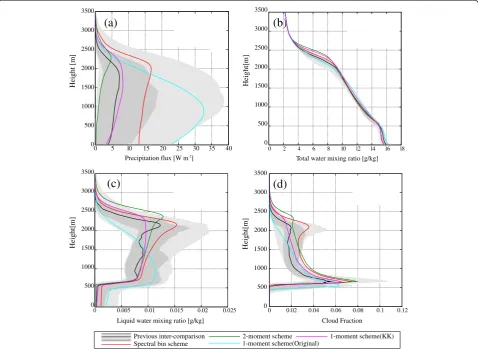
Second, we show the results of the same simulation (RICO) by using three microphysical schemes for inves-tigating the impacts of the cloud microphysical scheme. Figure 3 indicates the differences among the three schemes. The precipitation flux simulated by the two-moment bulk scheme is small, and its peak value is dis-tributed in the upper layer. By contrast, the precipitation flux by the one-moment bulk scheme is large and the peak value locates in the lower layer. The precipitation by the spectral bin scheme is between the other two (Fig. 3a). The trend is consistent with the previous study (Figure 6a of van Zanten et al. 2011).
The impacts of the different cloud microphysical schemes on the vertical distribution of the precipitation flux, the liquid water mixing ratio (ql), and cloud fraction are clearly shown in Fig. 3a–c. The ql in the one-moment bulk scheme is distributed in the lower layer (the peak value is represented at z~ 900 m). Table 2 shows the surface precipitation averaged during the last
4 h for the three schemes. The precipitation amount in the one-moment bulk scheme is the largest, and the pre-cipitation begins earliest among the three. The surface precipitation over 0.1 W m−2starts at 1.8 h in the one-moment bulk scheme, at 10.05 h in the two-one-moment bulk scheme, and at 2.63 h in the spectral bin scheme. The liquid water simulated in the two-moment bulk scheme is located in the upper layer (the peak value is located at z~ 2400 m), and only trace amounts of pre-cipitation reach the surface (Table 2). The cloud fraction of the one-moment scheme is located in the lower layer and is small in the upper layer. On the other hand, the positive cloud fraction in the two-moment bulk scheme reaches a higher layer. The spectral bin scheme simu-lates an intermediate value between the other two, with the same trend as the RICO study. These results are consistent with the result of the previous study (van Zanten et al. 2011).
The large amount of precipitation in the one-moment bulk scheme carries a large amount of liquid water to the lower layer. As shown in Fig. 3d, the total water mixing ratio (qt) of the lower layer (i.e., z< 1500 m) in the one-moment bulk scheme is larger than that in the others. Despite the difference in the vertical distribution of liquid water, the liquid water path (LWP) shows the same value (Fig. 3e). By contrast, the cloud coverage of the one-moment scheme is smaller than in the other scheme (Fig. 3f ). This implies that the amount of cloud that extends horizontally at the top of boundary layer is small in the one-moment scheme, which is because of the liquid water removed from the cloud layer earlier by precipitation. This is also found in Fig. 3c, where the peak of the cloud frac-tion does not appear around the top of the boundary layer (i.e.,z~ 2000 m).
(a)
(b)
(c)
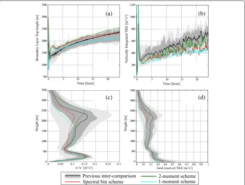
The impacts of cloud microphysics appear not only on the precipitation and vertical distribution of liquid water, but also the turbulent properties such as the turbulence kinetic energy (TKE), the variance in resolved vertical velocity (w’), and boundary layer top height. The bound-ary layer top height in the two-moment bulk scheme is the highest among the three schemes, whereas the one-moment bulk scheme simulates the lowest boundary
layer height. This trend in boundary layer height con-tinues to the end of the simulation time, as shown in Fig. 4a, and the difference among the schemes gradually becomes large. The variance in w’ (Fig. 4c) and TKE (Fig. 4d) in the two-moment bulk scheme attributes a larger value to the upper layer. By contrast, those in the one-moment scheme are smaller in the upper layer. Ver-tically integrated TKE tends to be large and small in the
(a)
(b)
(c)
(d)
(e)
(f)
(g)
(h)
(i)
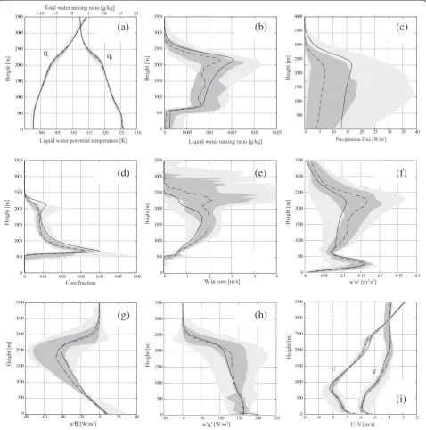
Fig. 2Comparison of vertical profiles between SCALE-LES and a previous intercomparison study. Horizontally averaged profile of thealiquid water potential temperature (θl) and total water mixing ratio (qt),bliquid water mixing ratio (ql),cprecipitation flux,dcloud fraction,evertical
velocity in cloud core,fvariance of resolvedw’,gw’θl’,hw’qt’, andihorizontal wind velocity, averaged during the last 4 h. Thesolid lineindicates
two-moment and the one-moment bulk schemes, re-spectively (Fig. 4b).
From the results shown above, we concluded that the turbulent properties of the boundary layer as well as the cloud microphysical properties of cumulus are signifi-cantly affected by the different microphysical schemes when other components are unchanged. These results
support the proposal of van Zanten et al. (2011) that the use of different cloud microphysical schemes is one of the main reasons for the diversity among LES models. We have confidence in this conclusion because direct ef-fects other than the cloud microphysical schemes were excluded in our experiments.
Reasons for the differences among the results of the three schemes
The impacts of the cloud microphysical schemes are clearly indicated by the differences in the boundary layer top height, vertical distribution of liquid water, and the precipitation flux, as shown in the previous section. The reasons for these differences will be discussed in this section.
Since the impacts of each cloud microphysical scheme originate from the expression of the liquid water in each scheme, an examination of the tendency ofqland poten-tial temperature (θ) in the cloud microphysical process
Table 1Computational performance of SCALE-LES
Number of core 16 2048 8192 32,768 131,072 663,552a
(Number of MPI process)
(2) (256) (1024) (4096) (16,384) (82,944)
Elapsed time (s step−1) 2.528 2.172 2.443 2.017 1.995 2.113
Performance efficiency (%)
5.5 6.3 5.6 6.8 6.9 6.5
Elapsed time (s step−1
) and performance efficiency (%) of SCALE-LES measured using the two-moment bulk microphysical scheme. The performance was measured through an experiment in which the number of grids for each MPI process was the same (weak scaling test) on the K computer
a
This test used all nodes of the K computer
(a)
(b)
(c)
(d)
(e)
(f)
is helpful for understanding the differences among the re-sults. We first investigate the difference duringt= 3−4 h of the calculation, because the effects of feedbacks of cloud physics to dynamics is not large and it is easy to interpret the difference. The tendencies at each height averaged duringt= 3 h tot= 4 h are shown in Fig. 5a, b. The results fromt= 0 h tot= 3 h were removed to ignore the effects of spin-up. The effect of sedimentation was omitted from the tendencies. The generation of liquid water at the cloud base in the one-moment bulk scheme is more active than that in the others (Fig. 5a). This is at-tributed to the difference in the mechanism for generating
cloud particles. In the one-moment bulk scheme, newly generated cloud particles are calculated by saturation adjustment, whereas in the other schemes, they are cal-culated based on Eq. (4). Because the saturation adjust-ment does not permit supersaturation, it can generate larger amounts of liquid water at the cloud base than that can be generated by the scheme based on Eq. (4), which allows for supersaturation. This large amount of liquid water generation results in a large heat release at the cloud base (Fig. 5b) and subsequently a strong vertical velocity (Fig. 5c).
In addition to the large amount of liquid water gener-ated in the one-moment bulk scheme, it is clear from the particle size distribution that the conversion from cloud to rain is fast. Size distributions at the lower part of cloud (i.e.,z= 1000 m) are shown in Fig. 5d. The gen-eration of drizzle and raindrops (i.e., particles over 40μm in radius) in the lower part of the cloud is active in the one-moment bulk scheme, whereas small cloud
Table 2Comparison of surface precipitation flux. The surface precipitation flux averaged over the whole calculation domain during the last 4 h of calculation
Scheme One-moment bulk Two-moment bulk Spectral bin
Precipitation flux
(W m−2) 22.89 0.174 13.17
(a)
(b)
(c)
(d)
particles are dominant in the two-moment bulk schemes. This indicates that the conversion from cloud to rain in the one-moment bulk scheme is faster than that in the others, and larger numbers of raindrops are generated in the lower part of the cloud by the one-moment bulk scheme.
The generation of large raindrops leads to the fast ter-minal velocity of the hydrometeors and a large precipita-tion flux in the one-moment bulk scheme (Fig. 5e), which, in turn, leads to the large precipitation flux at the surface and the fast onset of surface precipitation. Figure 5a, b also show that the peak negative tendency ofqlandθnear the cloud top (z~ 1700 m), which cor-responds to the evaporation of cloud droplets at the top of the boundary layer, is located in a lower layer in the one-moment scheme than in the others. This indicates that the large precipitation volume and large cloud size in the one-moment bulk scheme restrain the cloud particles from reaching the upper layer. Therefore, the boundary
layer top height of the one-moment bulk scheme becomes lower (Fig. 4a).
The large amount of raindrops in the one-moment scheme creates feedback for the thermodynamic struc-ture below the cloud. The water loading due to rain-drops leads to active evaporative cooling below the cloud (shown in the negative tendency ofqland θbelow the cloud as shown in Fig. 5a, b and the lower potential temperature below the cloud shown in Fig. 5f ). This evaporative cooling stabilizes the boundary layer and suppresses the heat transfer from the ground to the upper part of the boundary layer, which is shown in the fact that the positive tendency of θ in the one-moment bulk scheme does not reach z> 1200 m but reaches z~ 1400 m in the other scheme. This supports Stevens et al. (1998), who indicated that precipitation suppresses cloud growth and entrainment. This suppression can limit the development of the boundary layer and results in a more stable boundary layer.
0 500 1000 1500 2000 2500 3000 3500
Height[m]
Tendency of mixing ratio [mg/kg/s]
(a)
-0.04 -0.02 0 0.02 0.04 0.06 0.08 0.1 0.12
0 2 4 6 8 10 12
Precipitation flux [W/m2]
0 500 1000 1500 2000 2500 3000 3500
Height[m]
(e)
1e-10 1e-08 1e-06 0.0001 0.01 1 100
1 10 100 1000 10000
Number density (n(log m)) [# cm
-3]
Radius [µm]
(d)
-0.0001 -5e-05 0 5e-05 0.0001 0.00015 0.0002 0.00025 Tendency of potential temperature [K/s] 0
500 1000 1500 2000 2500 3000 3500
Height[m]
(b)
0 250 500
-2e-5 -1e-5 0 1e-5
0 500 1000 1500 2000 2500 3000 3500
296 298 300 302 304 306 308 310 312 314
Height [m]
Liquid water potential temperature [K]
0 250 500
296 298 300
(f)
0 500 1000 1500 2000 2500 3000 3500
0 0.02 0.04 0.06 0.08 0.1 0.12 0.14 0.16 0.18
Height [m]
w'w’ [m2/s2]
(c)
Spectral bin scheme 2-moment bulk scheme 1--moment bulk scheme z = 1000m
z = 1500m
The difference between the two-moment bulk and the spectral bin schemes in the tendency ofqlandθare rela-tively small. However, the difference in size distribution function between the two schemes is clearly apparent (Fig. 5d). A larger amount of raindrops (r> 100μm) were present in the spectral bin scheme than in the case in the two-moment bulk scheme. It is indicated that the conversion from cloud droplets to raindrops is slow in the two-moment bulk scheme. Because the amount of large raindrops is small in the two-moment bulk scheme (shown as green lines in Fig. 5d), liquid water is carried to the upper layer more easily than in the other schemes. The liquid water evaporates at the top of the boundary layer. This is shown by the negative tendency of ql, and byθ locating in a higher layer in the
two-moment bulk scheme than in the others (Fig. 5a, b). The presence of larger particles in the spectral bin scheme subsequently increases the rate of collisions with other particles, which leads to more rapid growth of par-ticles and earlier precipitation in the spectral bin scheme than in the two-moment bulk scheme. This provides feedback due to the large amount of precipitation, which is the same feedback that occurs in the one-moment bulk scheme.
With the feedback, the differences among the three schemes increase with the integration time. The differ-ence in the boundary layer top height in the three schemes becomes large as the integration time increases (Fig. 4a), and the difference in the liquid water potential temperature below clouds during the last 4 h (Fig. 3d) is larger than at t= 3–4 h (Fig. 5f ). The differences in the tendencies of θ and ql shown above also become clear (figure not shown).
In summary, the one-moment bulk scheme creates a larger amount of precipitation, because the saturation adjustment was adopted in the one-moment bulk scheme, and raindrops are subsequently produced by the fast cversion from cloud to raindrops. This results in earlier on-set and larger amounts of surface precipitation. The evaporative cooling by raindrops, which occurs actively below the cloud, stabilized the boundary layer in the one-moment bulk scheme.
The two-moment scheme creates raindrops more slowly, resulting in a smaller amount of precipitation compared with the other schemes. The smaller amount of precipita-tion results in an active latent heat release in the higher layer (shown in Fig. 5b) and a high boundary layer. The spectral bin scheme shows an intermediate rate of conver-sion and creates an intermediate amount of precipitation, with values between those of the two-moment and one-moment bulk schemes.
The large number of cloud particles newly generated at the cloud bottom by saturation adjustment, the difference in the speed of conversion from cloud to rain, and the
difference in the timing of the surface precipitation all ori-ginate from the variety of microphysical schemes used in this study. The differences in each scheme would not al-ways appear when the results of other one-moment, two-moment, and spectral bin schemes are compared. By con-trast, the evaporative cooling and subsequent stabilization of the sub-cloud layer and the suppression of the develop-ment of boundary layer height, which appeared in the re-sults of the one-moment scheme used in this study, can be expected if the fast conversion from cloud to rain or the active generation of cloud particles at the cloud base occurs as a result of natural phenomena, regardless of which scheme is used. The active latent heat release and high boundary layer, which appeared in the two-moment scheme used in this study, can also be expected. The re-sults are commonly expected for trade wind cumulus.
Speed of conversion from cloud to rain
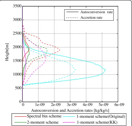
The analyses in the previous sections hint that the per-formance of the bulk microphysical schemes could be modified by changing the nucleation schemes and the conversion speed from cloud to rain. In the bulk scheme, autoconversion and accretion are the main processes volved in the conversion from cloud to rain. To obtain in-formation for the modification of the parameterization of these two processes, a comparison of the autoconversion and accretion rates among the three schemes is helpful. Figure 6 shows the autoconversion and accretion rates
0 500 1000 1500 2000 2500 3000 3500
0 1e-09 2e-09 3e-09 4e-09 5e-09 6e-09
Height[m]
Autoconversion and Accretion rates [kg/kg/s] Spectral bin scheme
2-moment scheme 1-moment scheme(KK) 1-moment scheme(Original)
Autoconversion rate Accretion rate
averaged during t= 3~4 h. The autoconversion rate of the spectral bin scheme is regarded as the rate of increasing mass of raindrops (defined as liquid parti-cles whose radius is larger than 40 μm) generated by the coagulation between cloud particles (defined as liquid particles whose radius is smaller than 40 μm). The accretion rate of the spectral bin scheme is de-termined as the increasing rate of mass due to the coagulation between cloud particles and raindrops. Figure 6 shows that the autoconversion rate of the one-moment scheme is about 15 times larger than that of the spectral bin scheme. By contrast, the ac-cretion rate of the two-moment scheme is 1.5~2 times smaller than that of the spectral bin scheme. Based on these results, the sensitivity of these two processes in each scheme was investigated and is dis-cussed in the next section.
Sensitivity of the autoconversion to the one-moment bulk scheme
As shown above, the one-moment bulk scheme overesti-mates the conversion speed from cloud droplet to rain-drop. We first investigated the difference between the original autoconversion scheme of Tomita (2008) and that of Khairoutdinov and Kogan (2000) shown in Eq. (6). The results of the one-moment bulk scheme with the Khairoutdinov and Kogan (2000) scheme are more similar to the results of the spectral bin scheme and the previous study than those calculated by Eq. (5) (Fig. 7). This indi-cates that the conversion speed calculated by Eq. (5) is too fast for shallow clouds because the validity of the one-moment bulk scheme with Eq. (5) was confirmed through experiments with deep convective clouds (Tomita 2008).
In addition to the experiment with the Khairoutdinov and Kogan (2000) scheme, other sensitivity experiments
0 5 10 15 20 25 30 35 40 0
500 1000 1500 2000 2500 3000 3500
Height [m]
(a)
Liquid water mixing ratio [g/kg]
0 500 1000 1500 2000 2500 3000 3500
Height[m]
Total water mixing ratio [g/kg]
(b)
0 0.005 0.01 0.015 0.02 0.025 0
500 1000 1500 2000 2500 3000 3500
Height[m]
(c)
Precipitation flux [W m-2]
0 2 4 6 8 10 12 14 16 18
0 0.02 0.04 0.06 0.08 0.1 0.12 0
500 1000 1500 2000 2500 3000 3500
Height[m]
(d)
Cloud Fraction
Previous inter-comparison 2-moment scheme 1-moment scheme(KK)
Spectral bin scheme 1-moment scheme(Original)
Fig. 7Cloud microphysical properties simulated by Khairoutdinov and Kogan’s auto conversion scheme. Horizontally averaged profile of the aprecipitation flux,btotal water mixing ratio (qt),cliquid water mixing ratio, anddcloud fraction averaged during the last 4 h. Thered,
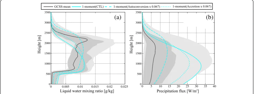
were conducted by reducing the autoconversion rate. Based on the analyses in Fig. 6, a 0.067-fold (i.e., 1/15) smaller autoconversion rate than the default value was used for the sensitivity experiment. Another sensitivity experiment with an accretion rate that was 0.067-fold smaller than the default value was also conducted. Figure 8 shows the profile of ql and the precipitation flux, which were calculated using the smaller autoconversion and ac-cretion rate. It can be seen that a small autoconversion rate results in liquid water locating in the upper layer, whereas it does not locate in the upper layer when the accretion rate was reduced to the same extent as the autoconversion rate. Hence, the autoconversion process is more sensitive to the production of raindrops.
Sensitivity of the accretion to the two-moment bulk scheme
Contrasting the one-moment bulk scheme, the two-moment bulk scheme underestimates the conversion speed from cloud to raindrop. We speculate that the fas-ter conversion from cloud droplet to raindrop in the two-moment scheme produced similar results using the spectral bin scheme. Sensitivity experiments were con-ducted by changing both the autoconversion and accre-tion rates of the two-moment scheme. Based on the analyses in Fig. 6, a twofold increase in the accretion rate was used, and a twofold increase of the autoconversion rate was also used for the sensitivity experiment. Figure 9 shows the results of these experiments. In the two-moment bulk scheme, both the precipitation rate and ql increase when the autoconversion rate is doubled. How-ever, doubling the autoconversion rate does not result in
a peak value of ql and a precipitation flux in the lower layer as simulated by the one-moment bulk scheme. By contrast, the precipitation flux simulated when the ac-cretion rate is doubled is considerably larger than both the default and when the autoconversion rate is doubled. This indicates that the accretion process was the major contributor to the creation of liquid water in the lower layer in the two-moment bulk scheme.
In short, the sensitivity of the accretion and the auto-conversion processes to the cloud microphysical proper-ties differ between the schemes.
Component level intercomparison
In this study, we investigated the exact effects of the various cloud microphysical schemes on model simula-tions of trade wind cumulus. If we change components other than the cloud microphysical scheme (e.g., dynam-ical core, turbulence scheme, advection scheme), the re-sponse of the cloud microphysical properties would change as suggested by van Zanten et al. (2011). It is ne-cessary to conduct sensitivity experiments by changing each component while keeping all other components fixed, as we did when targeting the cloud microphysical scheme in this study. We refer to these sensitivity exper-iments as a“Component level intercomparison”.
Grabowski (2014) suggested a piggyback approach to better understand the exact effects of cloud microphys-ics and the interaction between microphysmicrophys-ics and dy-namics. This approach can be also applied to the other components. Using a component level intercomparison and the piggyback approach, we can discuss the effects
(a)
(b)
0 500 1000 1500 2000 2500 3000 3500
0 500 1000 1500 2000 2500 3000 3500
0 5 10 15 20 25 30 35 40 0 0.005 0.01 0.015 0.02 0.025
Fig. 8Cloud microphysical properties simulated in the sensitivity experiment with a varying conversion ratio in the one-moment scheme. Horizontally averaged profile of thealiquid water mixing ratio (ql) andbprecipitation flux averaged during the last 4 h. Thesolid sky-blue,
of each component separately and obtain knowledge that would improve the parameterization of global scale models or regional models with coarse resolution.
Conclusions
In this study, we developed a large eddy simulation model (SCALE-LES), which excludes approximations and implicit schemes as much as possible. The results of a benchmark test indicated that SCALE-LES effectively reproduces the trade wind cumuli simulated in a previ-ous LES intercomparison study (van Zanten et al. 2011). Using SCALE-LES, we investigated the impacts of cloud
microphysical schemes on shallow cumulus and investi-gated which processes were critical for the diversity ob-served in previous LES intercomparison studies. Three types of cloud microphysical scheme, the one-moment bulk scheme of Tomita (2008), the two-moment bulk scheme of Seiki and Nakajima (2014), and the one-moment spectral bin scheme of Suzuki et al. (2010), were imple-mented with SCALE-LES for the sensitivity experiments.
The results indicated that the precipitation at the sur-face increases, in order, from the two-moment bulk scheme to the spectral bin scheme and the one-moment bulk scheme. Surface precipitation begins first in the 0
500 1000 1500 2000 2500 3000 3500
0 500 1000 1500 2000 2500 3000 3500
0 5 10 15 20 25 30 35 40 0 0.005 0.01 0.015 0.02 0.025
(a)
(b)
Fig. 9Cloud microphysical properties simulated in the sensitivity experiment with a changing conversion ratio in the two-moment scheme. The horizontally averaged profile of thealiquid water mixing ratio (ql) andbprecipitation flux averaged during the last 4 h. Thesolid green,dashed
green, anddotted green linesshow the results using the two-moment bulk scheme with the default autoconversion rate, two-moment bulk scheme with an autoconversion rate twice as large as the default, and two-moment bulk scheme with an accretion ratio twice as large as the default. Theblack line,dark gray shading, andlight gray shadingindicate the median, range between the first and third quartiles, and the range between the maximum and minimum values, respectively, for a previous intercomparison study (van Zanten et al. 2011)
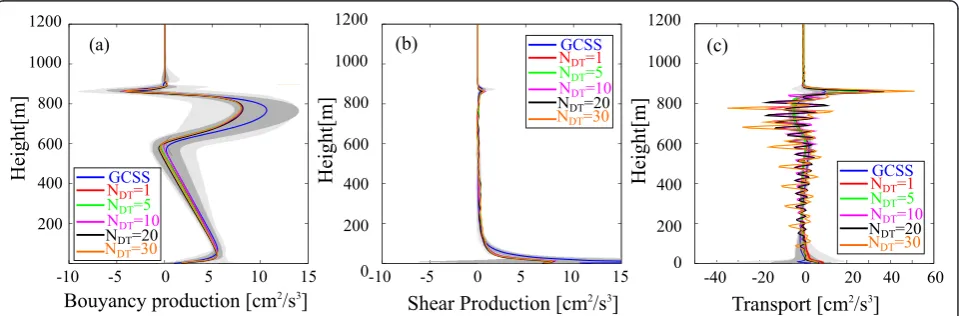
Fig. 10Cloud microphysical properties in the sensitivity experiment ofNDT(=Δtmicrophy/Δtdyn). Hourly averaged profile of theabuoyancy
production,bshear production, andctransport terms averaged over the entire calculation domain during the last hour of each simulation. The red,green,pink,black, andorange linesrepresent the results ofNDT= 1, 5, 10, 20, and 30, respectively. Theblue line,dark gray shading, andlight
one-moment bulk scheme, followed in order by the spectral bin and two-moment bulk schemes. These results support the suggestion of a previous intercomparison study (van Zanten et al. 2011)
Our analyses confirmed that the differences between the schemes were derived mainly from the generation of cloud particles and the speed of conversion from cloud droplets to raindrops. The differences in the two processes originated from the differences in the microphysical schemes used. By contrast, the phenomena generated by this variety, i.e., evaporative cooling and stabilization below the cloud and a low boundary layer, active latent heat release, and a high boundary layer can be expected regardless of the scheme used, if the active conversion from cloud to rain and the active generation of new cloud particles occur in nature.
The sensitivity of the autoconversion and accretion processes to the cloud microphysical properties simu-lated by the bulk microphysical schemes was also inves-tigated. In the two-moment bulk scheme the accretion process was more sensitive to the cloud microphysical properties, whereas the autoconversion was more sensi-tive in the one-moment bulk scheme. These results indi-cate that the tuning method of the microphysical scheme differs from scheme to scheme, and a compo-nent level intercomparison is useful to obtain the exact method for each scheme.
Appendix 1
Sensitivity of the ratio of the physical time step to the dynamical time step. In this study, the time step of dy-namics (Δtdyn), cloud microphysics (Δtmicrophy), and other physics (Δtphy) were set as 0.05, 0.15, and 0.5 s, re-spectively. The time step of dynamics was determined by the Courant–Friedrichs–Lewy (CFL) condition for the acoustic wave. The time step for physics (except for cloud microphysics) was set as 10 ×Δtdyn based on the sensitivity experiment (Nishizawa et al., 2015). The
Δtmicrophy was determined in sensitivity experiments examining the ratio of Δtmicrophy to Δtdyn. The results of the sensitivity experiments examining the ratioNDT (=Δtmicrophy/Δtdyn) are shown in this section. For this sensitivity test, the experimental setup of the second Dynamics and Chemistry of Marine Stratocumulus Re-search Flight 1 (DYCOMS-II RF01) (Stevens et al. 2005) was used. In this study, the experimental setup of the RICO study was used in most cases, but the effects of the acoustic wave appeared more clearly in the DYCOMS-II case (figure not shown). Consequently, the ratio (NDT) was determined using the DYCOMS-II RF01 experimental setup. For this sensitivity experiment, Δtdyn was set as 0.01 s andNDTwas swept from 1 to 30 (i.e.,Δtmicrophywas set from 0.01 to 0.3 s).
The results of the sensitivity experiment indicated that the effects ofNDT were mostly small (figures not shown), except for the TKE budget. Figure 10 shows the profile of the buoyancy production term, shear production term, and transport term of TKE production. The transport term was quite noisy when NDT was large (NDT> 10). Noise is also present in the shear production term. This noise was de-rived from the acoustic wave that was generated at every time step of the microphysical processes. WhenNDT was
Table 3List of non-dimensional coefficient for sensitivity experiment
Non-dimensional coefficient (γ) γ= 10−3
γ= 10−5
γ= 10−7
The strength of the numerical filter 1.25 × 10⁵ 1.25 × 10³ 1.25 × 101
The value of the numerical filter (m4 s−1
) for each experiment
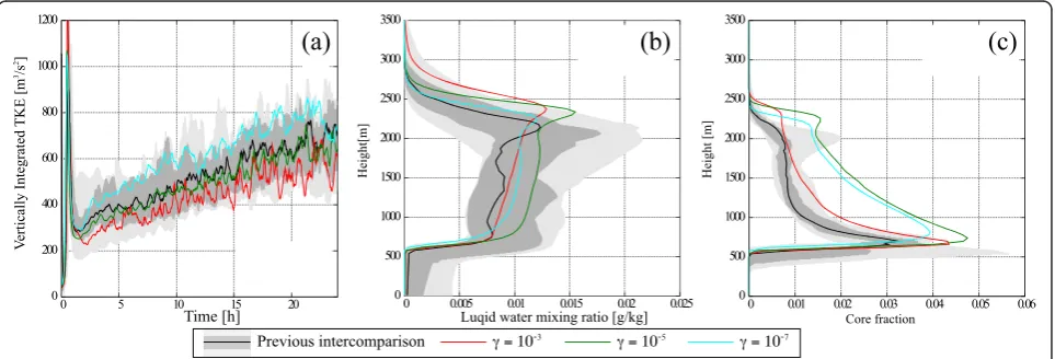
Fig. 11Results of a sensitivity experiment of the strength of numerical diffusion. Time evolution of theavertically integrated turbulence kinetic energy averaged over the whole calculation domain and the profile of thebliquid water mixing ratio andccloud fraction averaged over the whole calculation domain during the last 4 h. Thered,green, andsky-blue lineshows the results with the coefficient (γ) as 10−3, 10−5, and 10−7,
large, the variation ofθ at each step of the microphysical processes was also large. The large variation inθgenerates an acoustic wave, which produced the noise. This indi-cates that NDT should be smaller than 5 to render the effects of the acoustic wave negligibly. From these results and for safety,NDTwas set as 3 for the RICO experiment (i.e.,Δtmicrophy= 3 ×Δtdyn).
Appendix 2
Numerical filter. This section describes the sensitivity experiments of the strength of the numerical diffusion. Thenth ordered superviscosity/diffusion is defined as:
∂ ∂x νρ
∂n−1f
∂xn−1 2 4
3
5 f∈fu;v;w;θ;qsg:
∂ ∂x ν
∂n−1ρ
∂xn−1 2 4
3 5
Thevis written as:
ν¼ð Þ−1 n2þ1γ Δx
n
2nΔt
whereγis a non-dimensional coefficient,Δxis the grid spacing, and nis the order of the numerical filter. This study adopted a fourth-order numerical diffusion (i.e.,
n= 4) to dampen the artificial noise.nwas set as 4 be-cause of the computational efficiency.
To investigate the sensitivity of the strength of the numerical diffusion, simulations of the RICO study were conducted while changing the strength of the numerical diffusion. Based on the rough estimation of Nishizawa et al. (2015), the non-dimensional coefficient (γ) should be smaller thanO(10−3)–O(100) forn= 4. Thus,γwas chan-ged from 10−3to 10−7. The strength of the numerical diffu-sion for eachγis shown in Table 3. The two-moment bulk scheme was used for the sensitivity experiment. As a result of the numerical diffusion, one-dimensional sinusoidal two-grid noise will decay to 1/ewith a 1/γtime step.
Figure 11 shows the results of the sensitivity experi-ment. The vertically integrated TKE increased with a weakening of the numerical filter, even though the TKE of all experiments was located in the range between the maximum and minimum of the previous studies. This is because a strong numerical diffusion can efficiently dampen small-scale turbulence. As well as the TKE, the liquid water mixing ratio of all the sensitivity experi-ments was also located in the range of previous inter-comparison studies regardless of the strength of the numerical diffusion. However, the cloud fraction simu-lated with a small numerical diffusion (i.e., γ≤10−5) was much larger than that of the intercomparison study, and the cloud fraction was completely outside
the range of the inter comparison studies. The cloud fraction, core fraction, and variance of w’ were also outside the range of the inter comparison studies when γ was smaller than 10−5 (figure not shown). The temporal evolution of the cloud fraction indi-cates that the large cloud fraction, with small numer-ical diffusion, seems to originate from artificial noise. However, it is difficult to identify the reason for the large cloud fraction being artificial noise. The same experiment must be conducted with a fine grid reso-lution to divide all of the elements of the wave into a physically meaningful wave and artificial noise. However, computational limitations prevented us from conducting these experiments. Consequently, γ was determined using the results of the intercompar-ison study (van Zanten et al. 2011) as a reference so-lution, and γ was set as 10−3 (i.e., the strength of the numerical diffusion is 1.25 × 10⁵m4s−1).
Abbreviations
DYCOMS:Dynamics and Chemistry of Marine Stratocumulus; GCSS: GEWEX Cloud System Study; GEWEX: Global Energy and Water Exchange project; KiD: the kinematic driver; LES: large eddy simulation; LWP: liquid water path; MPI: Message Passing Interface; RICO: Rain in Cumulus over the Ocean; SCALE: Scalable Computing for Advanced Library and Environment; TKE: turbulence kinetic energy.
Competing interests
The authors declare that they have no competing interests.
Authors’contributions
YS implemented the cloud microphysical schemes in the SCALE library, designed this study, conducted the numerical simulations, analyzed the results of the simulations, and developed the manuscript. SN, HY, and YM developed the main frames of the SCALE library. YK collaborated with the corresponding author in the creation of the manuscript. HT proposed the development of the SCALE library. All authors read and approved the final manuscript.
Acknowledgement
Part of the results is obtained by the K computer at the RIKEN Advanced Institute for Computational Science. This work was supported by FOCUS Establishing Supercomputing Center of Excellence. SCALE-LES developed by Team-SCALE of the RIKEN Advanced Institute for Computational Sciences. The data from GCSS intercomparison studies used in several figures were downloaded from http://www.knmi.nl/samenw/rico/.
Received: 23 February 2015 Accepted: 6 August 2015
References
Ackerman AS, van Zanten MC, Stevens B, Savic-Jovcic V, Bretherton CS, Chlond A, Golaz J-C, Jiang H, Khairoutdinov M, Krueger SK, Lewellen DC, Lock A, Moeng C-H, Nakamura K, Petters MD, Snider JR, Weinbrecht S, Zulauf M (2009) Large-eddy simulations of a drizzling, stratocumulus-topped marine boundary layer. Mon Weather Rev 137:1083–1110. doi:10.1175/2008MWR2582.1
Berry EX (1968) Modification of the warm rain process. In: Proceeding of First Conference on Weather Modification., pp 81–85
Bretherton CS, Park S (2009) A new moist turbulence parameterization in the Community Atmosphere Model. J Clim 22:3422–3448. doi:10.1175/2008JCLI2556.1 Brown AR, Derbyshire SH, Mason PJ (1994) Large-eddy simulation of stable
atmospheric boundary layers with a revised stochastic subgrid model. Q J R Meteorol Soc 120:1485–1512. doi:10.1002/qj.49712052004
Considine G, Curry JA, Wielicki B (1997) Modeling cloud fraction and horizontal variability in marine boundary layer clouds. J Geophys Res 102:13517. doi:10.1029/97JD00261
Grabowski WW (2014) Extracting microphysical impacts in large-eddy simulations of shallow convection. J Atmos Sci 71:4493–4499. doi:10.1175/JAS-D-14-0231.1
Iguchi T, Nakajima T, Khain AP, Saito K, Takemura T, Suzuki K (2008) Modeling the influence of aerosols on cloud microphysical properties in the east Asia region using a mesoscale model coupled with a bin-based cloud microphysics scheme. J Geophys Res 113:D14215. doi:10.1029/2007JD009774
Kain, JS (2004) The Kain–Fritsch convective parameterization: An update. J Appl Meteorol. doi:10.1175/1520-0450(2004)043<0170:TKCPAU>2.0.CO;2 Khain AP, Sednev I (1996) Simulation of precipitation formation in the Eastern
Mediterranean coastal zone using a spectral microphysics cloud ensemble model. Atmos Res 43:77–110. doi:10.1016/S0169-8095(96)00005-1 Khairoutdinov M, Kogan Y (2000) A new cloud physics parameterization in a
large-eddy simulation model of marine stratocumulus. Mon Weather Rev 128:229–243. doi:10.1175/1520-0493(2000)128<0229:ANCPPI>2.0.CO;2 Naud CM, Del Genio AD, Bauer M, Kovari W (2010) Cloud vertical distribution
across warm and cold fronts in cloudsat-CALIPSO data and a general circulation model. J Clim 23:3397–3415. doi:10.1175/2010JCLI3282.1 Nishizawa S, Yashiro H, Sato Y, Miyamoto Y, Tomita H (2015) Influence
of grid aspect ratio on planetary boundary layer turbulence in large-eddy simulations. Geosci Model Dev Discuss 8:6021–6094. doi:10.5194/gmdd-8-6021-2015
Posselt R, Lohmann U (2008) Introduction of prognostic rain in ECHAM5: design and single column model simulations. Atmos Chem Phys 8:2949–2963. doi:10.5194/acpd-7-14675-2007
Pruppacher, HR, and Klett, JD, 1997, Microphysics of Clouds and Precipitation, 2nd ed., Kluwer Academic Publisher, Dordrecht, The Netherlands, 954pp. Randall DA, Coakley JA, Lenschow DH, Fairall CW, Kropfli RA (1984) Outlook for
research on subtropical marine stratification clouds. Bull Am Meteorol Soc 65:1290–1301. doi:10.1175/1520-0477(1984)065<1290:OFROSM>2.0.CO;2 Savic-Jovcic V, Stevens B (2008) The structure and mesoscale organization of
precipitating stratocumulus. J Atmos Sci 65:1587–1605. doi:10.1175/2007JAS2456.1
Scotti A, Meneveau C, Lilly DK (1993) Generalized Smagorinsky model for anisotropic grids. Phys Fluids A Fluid Dyn 5:2306–2308. doi:10.1063/1.858537 Seifert A, Beheng KD (2001) A double-moment parameterization for simulating
autoconversion, accretion and self collection. Atmos Res 59–60:265–281. doi:10.1016/S0169-8095(01)00126-0
Seiki T, Nakajima T (2014) Aerosol effects of the condensation process on a convective cloud simulation. J Atmos Sci 71:833–853.
doi:10.1175/JAS-D-12-0195.1
Shipway BJ, Hill AA (2012) Diagnosis of systematic differences between multiple parametrizations of warm rain microphysics using a kinematic framework. Q J R Meteorol Soc 138:2196–2211. doi:10.1002/qj.1913
Siebesma A, Bretherton CS, Brown A, Chlond A, Cuxart J, Duynkerke P, Jiang H, Khairoutdinov M, Lewellen D, Moeng C-H, Sanchez E, Stevens B, Stevens DE (2003) A large-eddy simulation intercomparison study of shallow cumulus convection. J Atmos Sci 60:1201–1219.
doi:10.1175/1520-0469(2003)060<1201:AALESIS>2.0.CO;B2
Stevens B, Cotton WR, Feingold G, Moeng C-H (1998) Large-eddy simulations of strongly precipitating, shallow, stratocumulus-topped boundary layers. J Atmos Sci 55:3616–3638. doi:10.1175/1520-0469(1998)055<3616:LESOSP>2.0.CO;2 Stevens B, Moeng C-H, Ackerman AS, Bretherton CS, Chlond A, de Roode S,
Edwards J, Golaz J-C, Jiang H, Khairoutdinov M, Kirkpatrick MP, Lewellen DC, Lock A, Müller F, Stevens DE, Whelan E, Zhu P (2005) Evaluation of large-eddy simulations via observations of nocturnal marine stratocumulus. Mon Weather Rev 133:1443–1462. doi:10.1175/MWR2930.1
Stocker, TF, Qin D, Plattner G-K, Tignor M, Allen SK, Boschung J, Nauels A, Xia Y, Bex V, and Midgley PM (2013), IPCC, 2013: Climate Change 2013: The Physical Science Basis, Cambridge University Press, Cambridge, United Kingdom and New York, NY, USA.
Suzuki K, Nakajima T, Nakajima TY, Khain A (2006) Correlation pattern between effective radius and optical thickness of water clouds simulated by a spectral bin microphysics cloud model. SOLA 2:116–119. doi:10.2151/sola.2006-030
Suzuki K, Nakajima T, Nakajima TY, Khain AP (2010) A study of microphysical mechanisms for correlation patterns between droplet radius and optical
thickness of warm clouds with a spectral bin microphysics cloud model. J Atmos Sci 67:1126–1141. doi:10.1175/2009JAS3283.1
Suzuki K, Nakajima T, Numaguti A, Takemura T, Kawamoto K, Higurashi A (2004) A study of the aerosol effect on a cloud field with simultaneous use of GCM modeling and satellite observation. J Atmos Sci 61:179–194.
doi:10.1175/1520-0469(2004)061<0179:ASOTAE>2.0.CO;2
Tiedtke M (1993) Representation of clouds in large-scale models. Mon Weather Rev 121:3040–3061. doi:10.1175/1520-0493(1993)121<3040:ROCILS>2.0.CO;2 Tomita H (2008) New microphysical schemes with five and six categories by
diagnostic generation of cloud ice. J Meteorol Soc Japan 86A:121–142. doi:10.2151/jmsj.86A.121
van Zanten MC, Stevens B, Nuijens L, Siebesma AP, Ackerman AS, Burnet F, Cheng A, Couvreux F, Jiang H, Khairoutdinov M, Kogan Y, Lewellen DC, Mechem D, Nakamura K, Noda A, Shipway BJ, Slawinska J, Wang S, Wyszogrodzki A (2011) Controls on precipitation and cloudiness in simulations of trade-wind cumulus as observed during RICO. J Adv Model Earth Syst 3:M06001. doi:10.1029/2011MS000056
Wang H, Feingold G (2009) Modeling mesoscale cellular structures and drizzle in marine stratocumulus. Part II: the microphysics and dynamics of the boundary region between open and closed cells. J Atmos Sci 66:3257–3275. doi:10.1175/2009JAS3120.1
Wang H, Feingold G, Wood R, Kazil J (2010) Modelling microphysical and meteorological controls on precipitation and cloud cellular structures in Southeast Pacific stratocumulus. Atmos Chem Phys 10:6347–6362. doi:10.5194/acp-10-6347-2010
Xue H, Feingold G, Stevens B (2008) Aerosol effects on clouds, precipitation, and the organization of shallow cumulus convection. J Atmos Sci 65:392–406. doi:10.1175/2007JAS2428.1
Yamaguchi T, Randall DA (2012) Cooling of entrained parcels in a large-eddy simulation. J Atmos Sci 69:1118–1136. doi:10.1175/JAS-D-11-080.1 Zalesak ST (1979) Fully multidimensional flux-corrected transport algorithms for
fluids. J Comput Phys 31:335–362. doi:10.1016/0021-9991(79)90051-2
Submit your manuscript to a
journal and benefi t from:
7Convenient online submission
7Rigorous peer review
7Immediate publication on acceptance
7Open access: articles freely available online 7High visibility within the fi eld
7Retaining the copyright to your article