Remittances, savings and return migration under uncertainty

O R I G I N A L A R T I C L E

Open Access

Remittances, savings and return migration

under uncertainty

Matthieu Delpierre

and Bertrand Verheyden

*Correspondence: [email protected] 1CEPS/INSTEAD, Esch-sur-Alzette, G.D. Luxembourg

Full list of author information is available at the end of the article

Abstract

Recent empirical evidence links migrant remittances, savings and return migration, and stresses the inaccuracy of return migration plans. This paper presents a model of endogenous remittances, savings and return decisions under uncertainty. In our framework, migrants make remittance and saving decisions at an early stage of migration, when their long term economic performance in the host country is still uncertain. Over time, information about professional prospects is acquired, and conditionally on past decisions, migrants adjust their return plans. We show that when migrants expect large gains from migration and face relatively low wage risks in the host country, they tend to remit less, save more and are less likely to return migrate. These results are in line with recent empirical evidence and provide a rationale for the support by relatives in the sending country of low-skill, illegal migration.

JEL codes: D13; D80; JE

Keywords: Remittances; Savings; Risk; Return migration

1 Introduction

Over the last decade, migrant remittances have become a key element of many develop-ing economies. In 2012, remittances represented a quarter of the GDP’s of countries such as Moldova, Lesotho and Nepal, and reaching even half of Tajikistan’s GDP.1_Remittances

are also important because their growth is both faster and more stable than official aid. For instance, the average annual growth rate of remittances to Sub-Saharan Africa has amounted to 13.9% over the 1995–2010 period.2These transfers help recipients in coun-tries of origin to cope with adverse shocks, and foster investments in various domains, such as education, productive assets and innovative technologies, but also in financial development, housing and social capital.3

In the face of such a major phenomenon benefiting recipient countries, economists have analyzed migrants’ behavior, and in particular their motivations to send remittances. Migrant altruism towards the family left behind is among the most widely acknowledged motives for remittances. Practically all other motives can be related to the existence of some implicit contract between the migrant and the recipient. Such contracts involve mutual insurance and various forms of investments made by migrants in the country of origin, in human, physical, financial and social capital.

Although this literature is relatively vast, the analysis of the motives for remittances has until recently overlooked important elements of the migrant’s decision process. While

the link between remittances and return migration plans has recently been observed, the-oretical analysis of the motives for remittances under endogenous return migration is scarce. More importantly, empirical studies show strong discrepancies between planned and actual duration of stay in the host country, due to uncertainty about their professional prospects and about their capacity to assimilate in the host country. Yet, theoretical analy-ses assume perfect foresight by migrants. Finally, a proper analysis of migrants’ remittance behavior should include alternative strategies of transferring resources to the future, such as savings, whereas theoretical and empirical studies generally analyze either remittances or savings, but not both. Addressing the following questions may therefore improve our understanding of migrants’ remittance and return migration strategies. Are migrants more or less likely to remit or to save under uncertainty? How do prior beliefs in terms of expected gains and risks from migration affect migrants’ remittance-saving portfolio? How do these decisions interact with labor market performance in the host country?

In this paper, we present a model of endogenous remittances, savings and return decisions under uncertainty. Remittances foster investments in the host country, and these investments also benefit the migrant.4 In our setting, migrants make remittance and saving decisions at an early stage of migration, when both labor market perfor-mance and return options are uncertain. Over time, when information about professional prospects is acquired, and conditionally on past savings and remittances, migrants choose to become either a permanent migrant or a return migrant by comparing the consump-tion levels they would obtain in each locaconsump-tion. It must be noted that this setting is in line with long-term international migration rather than circular migration.5

Savings and remittances are two technologies to transfer resources to the future, but they differ in some important aspects. When migrants consider whether to stay in the host country or return, they view savings as completely mobile, in the sense that these may be withdrawn and used in either location. In contrast, remittances lead to investments which have location-specific returns. Indeed, a migrant eventually opting for a perma-nent stay in the host country will only enjoy part (if any) of the remittance investment. For instance, investments in physical capital (e.g. houses, small businesses, inheritance,. . . ) will incur transaction costs to be repatriated in the host country. Other types of invest-ments in the origin country, for example in social capital (prestige, social status) are simply immobile and illiquid and therefore sunk. These considerations have strong implications in terms of return plans under uncertainty. For instance, we show that migrants who tend to remit large amounts in the early stages of migration have, ceteris paribus, a higher probability of return. Also, ex-ante, returns to remittances are random since they depend on the uncertain final location. In other words, unlike savings, remittances affect the dis-tribution of future consumption through (i) their different returns in each location and (ii) their impact on return migration.

are for instance legal migrants with low levels of education, and student migrants, whose returns from migration are potentially high but risky. Also, the model reproduces a series of recent stylized facts, linked to the determinants of remittance behavior, to the rela-tionship between remittances and return intentions, and to the economic performance of returnees.

First, all empirical analyses of remittance behavior highlight the existence of a large share of non-remitting migrants. Bettin et al. (2012) develop an econometric model which distinguishes various reasons for not remitting, either due to credit constrains, or due to the mere non-willingness to remit. Our framework captures these different possibilities, and explains why some unconstrained migrants may prefer not to remit. Since remit-tances increase the likelihood of return migration ex ante, and remitremit-tances have a higher return in the country of origin, returns to remittances are potentially convex. This con-vexity is a source of corner solution in remittances. Also, migrants who ex ante have high expectations about their economic outcomes in the host country are less likely to return. Because of this, they are also more likely to bear transaction costs to repatriate returns to remittances, which limits the attractiveness of such a form of investment. An additional reason for not remitting is related to the location of risks in host and origin countries. Migrants facing relatively low risk in the host country have no incentives to remit, as remitting affects the probability of return, and as a result increases the exposure to risks from the origin country. Conversely, this result is consistent with the observa-tion that migrants facing high uncertainty in the host country are more likely to remit (Amuedo-Dorantes and Pozo 2006; Sinning 2011).

The arguments on the impacts of expected gains and risks from migration provide a rationale for the important flows of illegal migration and their support by family members in developing countries. Indeed, our results imply that it is in the interest of migrants with low/risky prospects to remit. Therefore, relatives financing the migration of this type of agents are likely to receive transfers, independently of any pressure mechanisms.7_These

results are strongly related in our model to the positive effect of past remittances on the likelihood of return. Dustmann and Mestres (2010) prove the existence of this “feedback effect” in their thorough analysis of the impact of return plans on remittances. They show that failing to take it into account leads to biased estimates of that impact.

Finally, the empirical literature provides mixed evidence on the economic performance of return migrants. Our model provides rationales for this phenomenon, and may explain cases of negative selection of return migrants. For instance, Coulon and Piracha (2005) and Campos-Vazquez and Lara (2012) show that the average counterfactual wages of return migrants had they never migrated are lower than the average wages of stayers, despite the existence of a migration premium derived from the human capital accumu-lated in the host country. In our model, there is first a potential negative selection at the first stage of migration since, as explained above, migrants who have relatively low and risky benefits from migration are the most likely to remit, and therefore are likely to receive support. Second, because of transaction costs, the more migrants remit, the more they are ready to concede low wages in the origin country. Furthermore, the low prospect, high risk migrants are the most likely to remit and are therefore the most susceptible to return and earn low wages.

remittances are larger than the returns to savings, we say that remittances are sent with a “pure investment motive”. Second, when the migrant’s risk structure across locations is such that remittances reduce the total variance of future consumption, remittances may be sent with a “precautionary investment motive”. Illegal migrants are particularly subject to this second motive.

The paper is organized as follows. A review of the recent literature is provided in Section 2. The general setting is introduced in Section 3. The case of risk neutral migrants is presented in Section 4, while the case of risk averse migrants is analyzed in Section 5. In Section 6, we provide an extension of the model allowing for differences in purchasing power between the host country and the origin country. Concluding remarks are provided in Section 7.

2 Review of the literature

This paper links three fields of the migration literature: the study of (i) the motives for remittances, (ii) return migration plans, and (iii) the role of uncertainty at the early stages of migration.

First, the literature analyzing the motives for remittances has been initiated by Lucas and Stark (1985). Recent surveys of this question are provided by Rapoport and Docquier (2006), Carling (2008) and Stark (2009). Remittances are generally motivated by altru-ism towards the left behind and/or by the existence of an implicit contract between the migrant and the recipient. This implicit contract can take various forms. Remittances may be part of a mutual insurance arrangement. Indeed, migration allows families to diver-sify their income sources (Stark and Levhari 1982) and remittances can be considered as insurance transfers to the family left behind (Choi and Yang 2007; de la Briere et al. 2002; Gubert 2002). Remittances may also be seen as the repayment by the migrant of an implicit loan which made the initial migration possible (Poirine 1997). As previously men-tioned, remittances also foster investments in education (Edwards and Ureta 2003; Yang 2008, 2009; Calero et al. 2009 and Alcaraz et al. 2012), productive assets (Adams 1998) and innovative production technologies (Mendola 2008), but also in financial development (Aggarwal et al. 2011), housing (Adams Jr and Cuecuecha 2010; Osili 2004), social capital (Gallego and Mendola 2013; Maggard 2004) and family prestige (Auriol and Demonsant 2012).

Whether altruism is involved or not in the migrant’s decision making process, these investments generally benefit both remittance recipients and migrants themselves, either in terms of physical or social capital. For instance, remittances maintain membership rights in home communities (Osili 2007) and generate the gratitude from recipients (Stark and Falk 1998). Remittances may also be sent to migrants’ extended family and friends in order to ensure the provision of services, such as the maintenance of migrants’ patri-mony, cattle and crops (Cox 1987). Finally, migrants may invest in their future inheritance by sending money to their parents and improve their position against their siblings (the so-called strategic bequest motive, observed by Hoddinott (1994), Schrieder and Knerr (2000) and de la Briere et al. (2002)).

More recent contributions relate return migration to long term strategies (Borjas and Bratsberg 1996), motivated either by “lifecycle” or “target earnings” considerations. Migrants caring about lifecycle consumption determine the length of their stay abroad by trading off higher (utility) costs of staying abroad, including differences in purchasing powers, for higher earnings in the host country (Djajic and Milbourne 1988; Dustmann 1997, 2003; Stark et al. 1997). An increase in wages may lead “lifecycle migrants” to stay longer in the host country. In contrast, migrants wishing to invest in their country of ori-gin need to accumulate sufficient “target earnings” before returning (Djajic 2010; Mesnard 2004). These savings often translate into entrepreneurial activities, which require liq-uidities and are more profitable if migrants acquired specific skills and human capital in the host country (Dustmann and Kirchkamp 2002; Dustmann et al. 2011). Compared to lifecycle consumption, “target earnings” considerations provide opposite predictions: higher wages in the host country allow migrants to reach the required level of savings faster, allowing them to shorten their stay in the host country. Yang (2006) uses exchange rate shocks to empirically test both theories and finds a larger support for the lifecycle theory.

As regards remittances, recent empirical evidence highlights the positive link between return intentions and remittances (Dustmann and Mestres 2010; William et al. 2011; Sinning 2011) and between return intentions and asset holdings by migrants in the origin country (Dustmann and Mestres 2011). Yet to the best of our knowledge, our model is the first to take into account this relation, and in particular the feedback effect of remittances on return plans (Dustmann and Mestres 2010).

Third, with regard to uncertainty, most theories analyzing migration duration assume that duration is decided at the beginning of the migration process, under perfect fore-sight. There is however strong evidence that migrants form erroneous expectations about available opportunities in the host country (Borjas and Bratsberg 1996) and about the length of their stay, for instance in case of illegal migration and/or of poor economic performance (Tunali 2000). van Baalen and Müller (2008) follow a sample of migrants from Southern Europe and Turkey over 21 years using the German Socioeconomic Panel. While a mere 2.7% declared their intention to stay more than 20 years in 1984, 39% were still in Germany in 2004. These inaccurate expectations cannot only be attributed to the initial phase of migration, as for each additional year in the host country, about 70% of immigrants revise upward the duration of their stay. At the same time, about 26% of migrants who initially declared their plan to stay permanently in Germany had left by 2004. Labour market trajectories affect return migration, as shown by Kirdar (2009) and Bijwaard (2014) who both find that migrant unemployment has a positive impact on return. In addition to return decisions, recent empirical studies show that uncer-tainties about income and legal status also positively affect saving and/or remittance behavior (Amuedo-Dorantes and Pozo 2006; Piracha and Zhu 2012; Sinning 2011). Yet, few theoretical works incorporate uncertainty. Galor and Stark (1991) assume that return itself is random and exogenous and show that the return probability induces migrants to save more than native-born individuals. Dustmann (1997) presents a model of sav-ings and optimal duration under uncertainty. However, these decisions are jointly made ex ante.

social capital (membership rights, gratitude, status). Interestingly, a self-interested behav-ior involving investments of this kind mimics the predictions of the altruism motive (Stark and Falk 1998), since both altruistic and self-interested migrants benefit more from helping poorer recipients. Regarding the comparison between lifecycle and tar-get earnings theories of return migration, our framework is more in line with lifecycle considerations, since high wages in the host country lower the likelihood of return migration. It is also worth noting that unlike many theoretical analyses previously cited, our model does not require differences in purchasing power or in preferences for con-sumption between host and home countries in order to motivate return migration.9 Instead, return migration is motivated here by the fact that for some migrants, remit-tances may have a higher return than savings, or may decrease future risks. Because of the feedback effect, remittances increase the willingness to return. In other words, return migration in our framework is driven by the comparison between savings and remittances and by the feedback effect. The results obtained in this case are qualita-tively equivalent to the main setting. Finally, while the few studies which account for uncertainty preclude any revision of return migration plans when information about the migration outcome is revealed, our setting allows migrants to choose their final location after the revelation of information. This feature is one of the main driving forces of our results.

3 The model

Let us consider a migrant who lives for two periods, notedt ∈ {1, 2}. At the beginning of period 1, the migrant has just arrived in the host countryhand earns a certain ini-tial wagew1 ≥ 0, but faces uncertainty about long term wage prospects, i.e. wages that

could be obtained by settling in the host country, or by returning to the origin country

oafter a migration experience. Formally, at the beginning of period 1, the migrant only knows the joint density function of period-2 wages in the origin and host countries, noted

k(wo,wh). Also, at this period, the migrant makes decisions on savingssand remittances r. Consumption in period 1 is written:

c1=w1−r−s. (1)

Savings, which are placed on a bank account in the host country, produceτs at the beginning of period 2. Remittances are invested in the country of origin in some form of (physical, financial, social) capital.10This investment produces a returnRl(r)for the

migrant in period 2, which depends on the migrant’s location decisionl∈ {h,o}.11Rl(r)

is location-specific because if migrants choose to stay in the host country, migrants only partially benefit from investments made in the country of origin. The loss incurred in case of permanent migration is either due to transaction costs borne to liquidate the asset (e.g. a house, a small business,...), or simply because some specific types of assets, like social capital, are immobile, illiquid and therefore sunk. As a result,Ro(r)≥Rh(r). Also,

let us defineDR(r) ≡Ro(r)−Rh(r)as the difference in returns to remittances between

temporary and permanent migration, or transaction costs, which increase with the value of the investment:D_R(r) >0.12

At the end of period 1, the migrant observeswo andwh. Based on this information,

consumption levels in both locations. Period-2 consumption levels if the migrant opts for the origin / host countries are respectively:

co =wo+Ro(r)+τs, (2)

ch=wh+Rh(r)+τs. (3)

Note that contrary to remittances and wages, savings are perfectly mobile, since they can be withdrawn and spent in any location.

Summing up, this setting highlights the trade-off between higher expected wages in the host country and higher returns to remittances in the origin country in a context of uncer-tainty. In thefirst period,the migrant decides on savings and remittances(s,r). In the

second period,wages in both locations (wo,wh) are observed by the migrant, who chooses

a locationl ∈ {h,o}. Solving backwards, we start by analyzing the second period’s prob-lem, namely the location choice, and derive its consequences on the (ex ante) likelihood of return migration in period 1 and on saving and remittance decisions.

3.1 Optimal location choice

The migrant chooses the location in which the consumption level is the highest, so that ex-post, period-2 consumptionc2= max{co,ch}. In this simple setting, this choice boils

down to comparing the difference in returns to remittances between origin and host countries,DR(r) ≡ Ro(r)−Rh(r), to the difference in wages between host and origin

countries,Dw≡wh−wo.13At this stage, note thatDR(r)is certain and depends on a past

endogenous variable, whereasDwis a random variate.

Lemma 1.In period 2, the migrant returns to the origin country if Dw<DR.

The condition for return migration simply comes from the comparison between co

andch:

co>ch⇐⇒wh−wo≡Dw<DR≡Ro−Rh.

Having determined the optimal location condition, we can now start the analysis of the migrant’s problem in period 1. In this period, wages, and consequently the wage gapDw,

are treated as random variables. Return migration is therefore uncertain, and depends on the distribution ofDw. Letf(Dw)denote the marginal density ofDw, wheref(Dw)= k(wo,wh) ι (wh,wo,Dw)dwodwh, whereι (wh,wo,Dw)=1 ifwh−wo =Dwandι=0

otherwise. The cumulative density function ofDwis notedF(Dw).

Lemma 2.In period 1, the probability of return migration, Pr(Dw≤DR) = F(DR), increases with remittances:

∂F(DR)

∂r =f(DR)D

R(r) >0.

return migration, they have complex effects on the distribution of consumption patterns in period 2. These effects pertain to expected consumption on the one hand, and risk on the other hand. For the sake of expositional simplicity, we will separate the cases of risk neutrality and risk aversion in two distinct sections. In order to do so, recall first that the migrant’s preferences have two relevant aspects, namely risk aversion and consumption smoothing over time, which standard expected utility does not allow to disentangle.15 In contrast, the more general non-expected utility theory developed by Selden (1978) and Kreps and Porteus (1978) separates risk aversion and consumption smoothing.16 Following this approach, the migrant’s utility is noted

U=u(c1)+δu

g−1Eg(c2)

, (4)

where both u(·) andg(·) are increasing, concave functions.g−1Eg(c2)

= ˜c2is the

certainty equivalent functional of period-2 consumption, with

Eg(c2)=F(DR)E(g(co)|Dw≤DR)+(1−F(DR))E(g(ch)|Dw>DR), (5)

where with probabilityF(DR) the migrant returns to the country of origin and enjoys

E(g(co)|Dw ≤ DR), where co depends on the realization of wo. With probability (1−F(DR)), the migrant stays in the host country and enjoysE(g(ch)|Dw>DR). While

the concavity ofu(·)captures the migrant’s taste for consumption smoothing, the concav-ity ofg(·)captures the degree of risk aversion. Section 4 and 5 are based on two particular cases of Kreps-Porteus preferences. Section 4 covers the case of risk-neutral migrants hav-ing a taste for consumption smoothhav-ing, which corresponds to a linearg(·)function and a concaveu(·)function. This case allows us to introduce the “pure investment motive” for remittances, which appears when the expected return to remittances dominates that of savings. In Section 5, we introduce risk aversion by posing thatu(·)andg(·)are identical. This second case, which corresponds to expected utility, puts forward the “precaution-ary motive” for remittances: depending on the distribution of wage risks across locations, remittances may decrease the variance of future consumption.

4 Risk neutral migrant and the pure investment motive

Following equation (4) and using a linearg(·)function, the risk-neutral migrant’s utility is:

U=u(c1)+δu(E[c2]),

wherec1is defined in (1) andc2is equal toco(2) ifDw< DR, and is equal toch(3)

oth-erwise. SinceDwis by definition equal towh−wo, it belongs to the same data generating

process. Therefore, for a given pair(wo,wh) and its corresponding wage gapDw, the

fol-lowing joint densities have the same values:k(wo,wh)=m(wo,Dw)=n(wh,Dw), where m(wo,Dw)andn(wh,Dw)are joint densities of wages withDw.17Using these notations,

we can write the expectation of period-2 consumption by distinguishing the two final possible locations:

E[c2]= DR

−∞ +∞

−∞

(τs+Ro+wo)m(wo,Dw)dwodDw+ +∞

DR +∞

−∞

(τs+Rh+wh)n(wh,Dw)dwhdDw.

Let us first analyze the properties of the remittance technology in the way it affects the expectation of future consumption. Based on these properties, we will study in a second subsection the optimal remittances decision of risk-neutral migrants.

4.1 The impact of remittances on expected consumption

In this subsection, we will analyze the impact of remittances on (i) the expected consump-tion in each locaconsump-tion, and (ii) the total expectaconsump-tion of consumpconsump-tion, taking into account optimal location decisions.

The first analysis will provide interesting results about the economic performance of return migrants and of permanent migrants. In order to study the expected consumption in each location conditional, let us rewrite (6) as:

E[c2]=F(DR)E(co|Dw≤DR)+(1−F(DR))E(ch|Dw>DR), (7)

where conditional expectations of consumption in case of return and permanent migra-tion are respectively:

E(co|Dw≤DR)=τs+Ro+E(wo|Dw≤DR),

E(ch|Dw>DR)=τs+Rh+E(wh|Dw>DR),

and conditional expectations of wages are:

E(wo|Dw≤DR)= DR

−∞

⎛ ⎝

+∞

−∞

wom(wo|Dw)dwo

⎞ ⎠f(Dw)

F(DR)dDw,

E(wh|Dw>DR)= +∞

DR

⎛ ⎝

+∞

−∞

whm(nh|Dw)dwh

⎞

⎠ f(Dw) 1−F(DR)dDw.

This decomposition allows us to assess the impact of remittances on the expected con-sumption in each location separately, taking into account the endogeneity of the location decision. Such an exercise brings two interesting findings. First, it allows us to provide an explanation to the poor performance of some return migrants.18 Second, it shows that remittances, although they are more productive in case of return migration, increase the conditional expectation of consumption of migrants settling in the host country.

Proposition 1.Conditionally on optimal location decisions in period 2,

1. remittances decrease the expected wageE(wo|Dw≤DR), but have an ambiguous

impact on the expected consumption in the country of origin:

∂E(co|Dw≤DR)

∂r =R

o(r)+

∂E(wo|Dw≤DR)

∂r ,

whereR_o(r)≥0but∂E(wo|Dw≤DR) ∂r <0.

2. remittances have a positive impact on the expected wage and consumption in the host country:

∂E(ch|Dw>DR)

∂r =R

h(r)+

∂E(wh|Dw>DR)

∂r >0,

whereR_h(r) >0and∂E(wh|Dw>DR) ∂r >0.

Remittances have an ambiguous impact onE(co|Dw ≤ DR) because, ceteris paribus,

migrants who remit more are ready to concede lower wages in the origin country. Indeed, asrincreases, so doesDR, so that the condition to return (Dw≤DR) is easier to satisfy.

In other words, return migration is compatible with higher values ofDw, that is, lower

(higher) values ofwo(wh). This result provides a rationale for poor economic outcomes

of return migrants: the more migrants remit, the more likely they will return, and the lower the wages they are ready to accept in case of return. Conversely, remittances have a positive impact onE(wh|Dw > DR): migrants who remit are less likely to stay, which

implies that they will do so only for sufficiently large wages in the host country.

Having analyzed the impact of remittances by location, let us now analyze their global impact onE[c2]. To this end, let us rewrite (6) as:

E[c2]=τs+E[R]+E[w] , (8)

where:

E[w]≡F(DR)E(wo|Dw≤DR)+(1−F(DR))E(wh|Dw>DR), (9)

E[R]≡F(DR)Ro+(1−F(DR))Rh. (10)

E[w] is the expected wage, based on the distributions of wages in each location condi-tional on the wage gapDw. Similarly,E[R] is the total expectation of return to remittances,

which also depends on ex-post location decisions. In order to show the impact of remit-tances onE[c2], let us first analyze their impacts onE[w] andE[R] separately. The next

Lemma shows that migrants who decide to remit anticipate lower expected wages, but higher expected benefits from remittances.

Lemma 3. Remittances have a negative impact on E[w]and a positive impact on E[R]: ∂E[w]

∂r = −f(DR)D

RDR<0, ∂E[R]

∂r =f(DR)D

RDR+ER(r)>0, where

ER(r)≡F(DR)R_o(r)+(1−F(DR))R_h(r) >0. (11)

The first part of the lemma, which states that remittances have a negative impact on expected wages, is explained by the following intuition. Remitting increases the likelihood of return migration byf(DR)D_R. The global distribution of wages is unaffected by this change, except at the margin where migrants are indifferent between returning and stay-ing, i.e. whenDw=DR. When switching from staying to returning, they renege onwhto

earn a wagewo instead. Therefore, they suffer a lossDwat this marginal point, which is

precisely equal toDR.

The second part of the lemma highlights two positive effects ofronE[R]. The first effect stems from the fact that, as for E[w], remittances increase the likelihood of return migration at the margin. At this margin, migrants enjoy a returnRo(r)instead of Rh(r): they benefit from a marginal increase equal toDR. The second and most

obvi-ous term accounts for the marginal returns to remittances in each location,R_o(r)and

R_h(r). Weighting these two marginal returns by their respective probabilities leads to

Proposition 2.The total expectation of future consumption is increasing, and poten-tially convex in remittances.

∂E[c2]

∂r =

∂E[R]

∂r +

∂E[w]

∂r =E

R(r)>0,

∂2_E[c 2]

∂r2 =f(DR)

D_R(r)2+ER(r),

(12)

where

ER(r)=F(DR)R_o(r)+(1−F(DR))R_h(r).

Combining the two parts of Lemma 3 leads directly to Proposition 2. This proposition shows first that remittances affectE[c2] through an increase in returns to remittances,

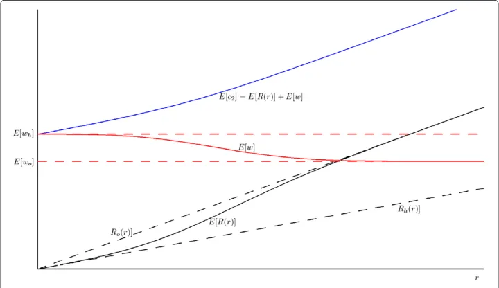
but also a decrease in the expected wage, since remittances increase the likelihood of migrating back to the country of origin, where wages are on average lower. How-ever, the net marginal effect of remittances on expected consumption is always positive, and corresponds to the expected marginal return to remittances, ER(r). Figure 1 illustrates these effects. In this figure, when remittances are close to zero, the proba-bility of return migration is zero, so thatE[R(r)] = Rh(r), andE[w] = E[wh].19 As

remittances increase, the likelihood of return migration becomes strictly positive, and

E[R(r)] increases, as it becomes a convex combination ofRh(r)andRo(r). Also,E[w]

decreases, as it depends on the distribution of bothwh andwo. As stated in the

previ-ous proposition, the sum of these two effects is always positive (the blue curve is always increasing inr). As remittances increase further, they become so large that the proba-bility of returning to the origin country becomes equal to 1. In that case,E[R(r)] =

Ro(r), and E[w] = E[wo]. Further increases in remittances no longer affect expected

wages, while returns to remittances are perceived with certainty in the country of origin.

Secondly, the proposition shows that expected consumption is not only increasing, but may also beconvexinr. This potential convexity comes from the first term in the right hand side of (12), which is positive and is due to the feedback effect of remittances. Indeed, even ifRo(r) andRh(r) are not convex, expected consumption may be more

and more increasing in remittances because the more the migrant remits, the higher the probability of returning to the origin country, where the benefits of remittances are the highest. In other words, as the migrant remits, E[R(r)] puts more weight on

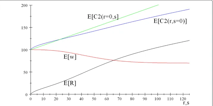
Ro(r), and less onRh(r). In Figure 2, we present a case whereRo(r)andRh(r)are both

linear, so that, following the previous reasoning, returns to remittances are always con-vex:∂2E[c2]

∂r2 =f(DR)

D_R(r)2≥0. Figure 2 illustrates that as long as remittances increase the likelihood of return migration,E[c2] is always convex in remittances whenRo(r)and Ro(r)are linear.

Figure 1 The remittance technology.

4.2 How migrant characteristics affect the impact ofronE[c2]

In this subsection, we discuss the impact of migrants’ and recipients’ characteristics on the shape of returns to remittances, both through ∂E[c2]

∂r and ∂

2_E[c2]

∂r2 . While we provide here analytical results and their interpretation, the interested reader can find graphical representations of these results based on calibrations of the model in Appendix 2.

First, we show that the higher the migrants’ anticipations about their labor market per-formance in the host country, the lower their expected marginal returns to remittances. In order to show this, let us consider that some migrants have higher wage prospects from migration than others following the concept of first order stochastic dominance. A migrant with high (low) wage prospects faces a cumulative distribution of the wage gap between host and origin countries notedFPh(Dw)(FPl(Dw)). The distribution of the wage

gap for migrants with high prospects first-order stochastically dominates that of migrant

with low wage prospects:FPh(Dw)≤FPl(Dw)for allDw. In other words, for any givenDw,

the higher the migrant’s wage prospects, the lowerF(Dw). Note that first order stochastic dominance implies that migrants with higher prospects have a higher expected wage gap:

EPh(Dw)≥EPl(Dw).

Lemma 4.For all r, the higher the migrant’s wage prospects, the lower ∂E[c2]

∂r .

Proof.One can rewrite ∂E[c2]

∂r = E

R(r) as F(DR(r))DR + Rh(r), which clearly

increases with F(DR(r)). For a given level of DR, a migrant with higher migration

prospects faces a lower expected marginal return to remittances. See Appendix 2 for a graphical illustration.

Let us now discuss how recipient characteristics affect∂2E[c2]

∂r2 . We have seen that∂ 2_E[c

2]

∂r2 is the sum of two terms,f(DR)D_R(r)2andER(r). While the first is always posi-tive, the second term may also be posiposi-tive, depending on the way recipients in the origin country use remittances. Indeed,ER(r)is more likely to be positive in poor receiving households than in rich ones. Intuitively, poor families are likely to first allocate remit-tances to their basic needs. The more the migrant remits, the higher recipients’ capacity to switch to more productive investments, which also benefits the migrant. Marginal returns to remittances are therefore negligible for low levels of remittances, and become attrac-tive as recipient households have improved their living conditions. As a result, migrants originating from poor households are more likely to face convex returns to remittances. This reasoning has been illustrated by Adams (1998), which shows that households with a migrant member have a higher marginal propensity to invest.

In the next section, we analyze migrants’ optimal saving and remittance decisions, taking into account the potential heterogeneity in the remittance technology across migrants.

4.3 Optimal savings and remittances under risk neutrality

The risk-neutral migrant’s objective is:

Max

{s,r} U=u(c1)+δu(E[c2]),

where c1 andE[c2] are defined in (1) and (8), and both rand s need to satisfy

non-negativity constraints. While remittances can obviously not be negative, borrowing is precluded by the migrant’s lack of credibility to repay a loan in case of return migration. As mentioned in Proposition 2, returns to remittances may either be concave, or convex. Let us analyze these two cases separately.

Proposition 3.Under risk neutrality, if∂2E[c2]

∂r2 ≤0, then three types of remittance-saving

portfolios are possible:(0,s∗),(r∗,s∗)and(r∗, 0), where:

• under “high” migration prospects (largeE[Dw]):(0,s∗)such that u₁

δu

2 =τ >E

R(0),

• under “intermediate” migration prospects:(r∗,s∗)such that u1

δu

2 =τ =E

• under “low” migration prospects (smallE[Dw]):(r∗, 0)such that u₁

δu 2 =E

R(r∗)> τ.

The migrant’s optimal strategy of saving/remittance portfolio is determined by the Kuhn Tucker conditions with respect to savings and remittances, which are respectively:

Us= −u1+δu2τ =0 ands>0,

= −u₁+δu₂τ <0 ands=0, (13)

and

Ur= −u1+δu2E

R(r)=0 andr>0, (14)

= −u₁+δu₂ER(r)<0 andr=0. (15)

If both first order conditions are satisfied with equality, that is, if there is an interior solution in bothrands, we obtain the following arbitrage condition:

ER(r)=τ. (16)

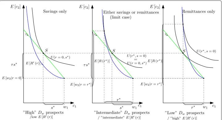
The marginal returns to both activities must equalize at this double interior solution. However, depending on the migrant’s wage prospects, one of these two first order condi-tions may not hold with equality, leading to a corner solution in eitherrors. Following Lemma 4, if prospects are so high thatER(0) < τ, marginal returns to remittances are too low for the migrant to send remittances ; instead he/she will focus on savings. In contrast, if prospects are low, the optimal level of remittances may still have a marginal return which dominates that of savings:ER(r∗)> τ. In this case, the migrant has no incentives to save and will only remit. These three cases are illustrated in Figure 3.

It must be noted that the solutions described here are valid if and only if ∂2E[c2]

∂r2 < 0. Intuitively, for the arbitrage condition,ER(r)=τ, to hold at equilibrium, remittances should have a decreasing expected marginal return. Indeed, remittances below the inte-rior solution should have a higher marginal return than savings, while remittances beyond

the interior solution should have a lower return than savings. If, as mentioned in the pre-vious section, remittances have an increasing marginal return, this reasoning does not hold, and a corner solution will prevail. As shown in the next proposition, the case of convex returns to remittances is incompatible with an interior solution in bothsandr.

Proposition 4.If ∂2E[c2]

∂r2 > 0, then the optimal remittance/saving portfolio of the

migrant is never diversified. Two remittance-savings portfolios are possible, (0,s∗) and (r∗, 0), where:

• under “high” migration prospects:(0,s∗)withU(0,s∗) >U(r∗, 0)ands∗such that

u₁ δu

2 =τ

,

• under “low” migration prospects:(r∗, 0)withU(r∗, 0) >U(0,s∗), andr∗such that

u₁ δu

2 =E

R(r∗).

Proof.See Appendix 3.

The main insight of this case is that the optimal remittance/saving portfolio of the migrant is never diversified when returns to remittances are convex. Which of the two assets is chosen depends again on return prospects. If prospects are high (low), marginal returns to remittances are low and the migrant saves (remits).

Figure 4 illustrates why an interior solution in bothsandris impossible under con-vex returns to remittances. On the left graph, for low values ofr, marginal returns to remittances are too low compared to returns to savings,τ. Remitting large amounts in order to enjoy high marginal returns to remittances would distort the migrant’s consump-tion path excessively (insufficient consumpconsump-tion in period 1) compared to the balance offered by savings (point S). The graph in the middle represents the limit case in which the migrant is indifferent between only saving (point S) and only remitting (U(r∗, 0) =

U(0,s∗)). In this case, due to the convexity of returns to remittances, the migrant needs to remit a larger amount than what he/she would have saved (r∗ > s∗) in order to reach

the attractive portion of returns to remittances.20 Finally, the last graph illustrates the case in which returns to remittances are large and/or very convex. Since marginal returns to remittances become quickly high, and the migrant only remits. Here, the migrant may consume more in period 1 than he/she would have with savings.

Let us now analyze the risk implications of remittances.

5 Risk averse migrants and the precautionary investment motive

In this section, we generalize migrants’ preferences by introducing risk aversion, while maintaining the rest of the model unchanged. As previously mentioned, the migrant’s utility function in this section is based on expected utility:

U=u(c1)+δEu(c2), (17)

wherec1is defined in (1) andc2is equal tocoifDR > Dw, and is equal tochotherwise,

wherecoandchare defined respectively in (2) and (3). In this analysis, we will make use

of the standard concepts of certainty equivalent and Arrow-Pratt approximation of the risk premium. Let˜c2denote the certainty equivalent ofc2, that is,u(˜c2) =Eu(c2). This

certainty equivalent can be approximated by

˜

c2≈E(c2)− η

2Var(c2), (18)

whereηis the migrant’s degree of absolute risk aversion. Based on this formula, and since we already studied the effect of remittances onE(c2), we will focus in this section on the

variance ofc2. One can show, as an application of the law of total variance, thatVar(c2)

takes the following form:

Var(c2)=E[Var(c2|Dw)]+Var[E(c2|Dw)] ,

where

E[Var(c2|Dw)]=F(DR)Var(wo|Dw≤DR)+(1−F(DR))Var(wh|Dw>DR), (19)

and

Var[E(c2|Dw)] = F(DR) (1−F(DR))[E(co|Dw≤DR)−E(ch|Dw>DR)]2

= F(DR) (1−F(DR))[DR+E(wo|Dw≤DR)−E(wh|Dw>DR)]2.

(20)

Let us describe intuitively the two terms composing the variance ofc2. The first term, E[Var(c2|Dw)], which is decomposed in (19), represents the average variance over the

two locations. More precisely, it is the weighted sum of consumption variances by loca-tion, where weights are the probabilities of choosing these respective locations. The second term,Var[E(c2|Dw)], which is decomposed in (20), represents the consumption

variance which is due to differences in expected consumption across locations. This sec-ond term can be interpreted as the risk imposed by the uncertainty about the future location itself.

5.1 The impact of remittances on consumption variance

In this section, we will provide a rationale, based on risk considerations, to the fact that migrants facing relatively more risks in the host country, such as illegal migrants, are more likely to remit than others. Indeed, the initial distribution of uncertainty is an important determinant of the migrant’s ability to use remittances as a precautionary investment. More precisely, we show that if the wage uncertainty is mostly located in the host country labor market, remittances have the property ofreducing future con-sumption variance. This argument also provides a rationale for the fact that in developing countries, families provide support for illegal/risky migration. Indeed, it is in the own interest of migrants facing high risk in the host country to send remittances, so that families are likely to receive a return on investment independently of pressure mecha-nisms, such as migrant networks. This section also allows us to show that the location choice (temporary versus permanent migration) is per se a risk-coping mechanism, used ex post. Remittances, sent ex ante, improve the effectiveness of this ex-post risk-coping device.

The impact of remittances on aggregate risk is highlighted in the following Lemma. The economic intuition follows in the subsequent propositions.

Lemma 5.The derivative of the total consumption variance is determined by

∂Var(c2)

∂r =2D

RF(DR) (1−F(DR))[E(co|Dw≤DR)−E(ch|Dw>DR)]

+f(DR)D_R[Var(wo|DR)−Var(wh|DR)] .

(21)

Proof.See Appendix 4.

Lemma 5 describes the effect of remittances on the variance of the migrant’s future consumption. The sign of this effect depends on two terms. First, remittances are likely to decreaseVar(c2)if the expected consumption is lower in the origin country than in

the host country (E(co|Dw ≤ DR) < E(ch|Dw > DR)). Note that these expectations are

conditional on the wage gap, and that the distribution of wages across the two locations is in fact a crucial determinant of the sign of this first term. Second, remittances are likely to decreaseVar(c2)if, at the margin where the migrant is indifferent between staying and

returning (i.e. forDw=DR), the variance of wages in the origin country is lower than the

variance of wages in the host country.

In order to provide more insights from this general formula and to highlight the role played by the distribution of wage risks across locations, we need to add more struc-ture on the distribution of wages. To this end, we will assume that wages are drawn from a bivariate normal distribution, with meansE[wo] = μo and E[wh] = μh and

variances Var[wo] = σo2 andVar[wh] = σ_h2. We assume without loss of generality

that wages are independently distributed across locations, so thatcov(wo,wh) = 0.21

The reason why we assume a bivariate normal distribution is that this distribution has appealing properties allowing analytical solutions and providing intuitive results. One implication of normality is that the migrant’s income variance is minimized for

E(co|Dw ≤ DR) = E(ch|Dw > DR). This is intuitive since, at this point,

from an insurance perspective (precautionary motive), remittances are also potentially sent to increase the migrant’s expected income (pure investment motive). This com-bination of motives is explored in the section devoted to the migrant’s optimization problem.

5.2 How migrant characteristics affect the impact ofronVar(c2)

As in the previous section, let us consider how some migrant characteristic may affect the remittance technology, in term of consumption variance this time. Let us define the relative variance of wages in the host country as

θh≡ σh2 σ2

o +σh2

∈[0, 1] .

Clearly, migrants differ in terms ofθh. For instance, illegal migrants are more likely to face risk in the host country, in which caseθhis close to one. On the other hand, well established and integrated migrants should face very little risk in the host country, while uncertainty in case of return is higher.

Proposition 5.Remittances are risk-reducing if the relative host-country wage variance θhis sufficiently large:

∂Var(c2)

∂r <0 ⇐⇒ θh>θh, (22)

where the thresholdθhdepends on DR(r):

_θh≡ DR−E(Dw|Dw≤DR)

E(Dw|Dw>DR)−E(Dw|Dw≤DR)) ∈

[0, 1] .

Proof.See Appendix 5.

Proposition 5 indicates that remittances decrease the aggregate income risk faced by the migrant if her initial risk is mainly located in the host country (largeθh). Intuitively, increasing remittances makes return migration more likely, which reduces the exposure to the relatively large risk in the host country. An important implication of Proposition 5 is thatθhis itself a function of the level of remittances. The next proposition states that the impact of remittances on risk is non-monotonic.

Proposition 6.θhis increasing in r. Therefore, Var(c2)is potentially non-monotonic in r, being decreasing for low r, and increasing for large r.

Proof.See Appendix 6.

initial geographical distribution of risks, the migrant is protected against low wages by the ability to select the best outcome among both locations. In other words, the migrant is capable of mitigating a negative shock in one location by moving to the other location. Moreover, as we show in the following example, this instrument is most powerful if risk is evenly distributed among locations. Example 1 provides the intuition behind proposi-tions 5 and 6, namely that remittances are risk-reducing if risk is mainly located in the host economy and that transferring too much risk towards the origin country might, at the end, increase the aggregate risk faced by the migrant. In order to illustrate these points, we use a simplified framework where the only decision variable is location.

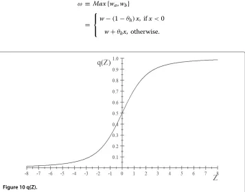
Example 1.Suppose an agent can choose between two locations{a,b}, where wages are random and take the following form:

wa=w−(1−θh)x,

wb=w+θhx,

where x∼F(x)and E(x)=0. Letω≡Max{wa,wb}define the wage the agent will obtain in period two after selection of the optimal location. Two results emerge from this example.

1. The capacity to choose the best location always improves the expected

consumption: the expected consumption conditional on optimal location,E(ω), is larger than the unconditional expected consumption w.

2. The consumption variance conditional on optimal location,Var(ω)is minimized when the initial income risk is identical in both locations, i.e. forθh=1/2.

Proof.See Appendix 7.

As this simplified example illustrates, on the one hand, the location choice allows the migrant to increase expected consumption. On the other hand, it shows that aggregate risk depends on the initial risk composition. More precisely, the more the distribution of wage risks across locations is even ex ante, the lower the variance of consumption conditional on optimal location. If risk is mainly located in the host economy, remittances can be used to improve the balance of risks across locations, so that aggregate risk is reduced. This mechanism provides an explanation to the empirical evidence according to which migrants facing higher risks in the host country are more likely to remit (Amuedo-Dorantes and Pozo 2006). On the contrary, as stated in Proposition 6, remittances may increase aggregate risk if the origin country is relatively riskier.

5.3 Optimal savings and remittances under risk aversion

The migrant maximizes expected utility with respect to savings and remittances. The first order conditions are given by

Us= −u1+δu2τ ≤0, (23)

Ur= −u1+δu2 ∂˜c2

∂r ≤0, (24)

where˜c2is defined in equation (18), so that under constant absolute risk aversion, ∂c˜2

∂r ≈ ∂E(c2)

∂r −

η

2

∂Var(c2)

where ∂E(c2)

∂r = E

R(r), as described in Proposition 2, and where the impact on the variance is given by equation (21). We are now able to formally take into account both precautionary and pure investment motives. Under risk neutrality, we have shown that returns to remittances are potentially convex, as discussed after equation (12). In the risk averse case, we need to also take into account the effect of remittances on consumption variance in order to define the concavity or convexity of total returns to remittances. Note that another source of migrant heterogeneity, namely risk aversionη, amplifies this result: the largerη, the larger the impact ofronVar(c2).

Definition 1. Under risk aversion, total returns to remittances are concave if

∂2_c 2 ∂r2 ≈

∂2_E(c 2) ∂r2 −

η

2

∂2_Var(c 2)

∂r2 ≤0. (25)

Whether returns to remittances are convex or concave matters for the optimal migrant portfolio. Indeed, as in the section with risk neutrality, we know that the migrant’s objec-tive may admit an interior maximum in bothsandronly if total returns to remittances are concave. Although convex total returns to remittances are still possible for risk averse migrants, this possibility is less likely than in the case of risk neutral migrants. The fact that concavity is more relevant under risk aversion than under risk neutrality is due to the impact of remittances on the variance of consumption. By Proposition 6, we know that ∂2Var(c2)

∂r2 > 0. This effect, whose magnitude increases with the degree of absolute risk aversionη, increases the likelihood of concave returns to remittances. As a result, it is likely that risk averse migrants choose strictly positive levels of both savings and remittances. However, one should keep in mind that, even if returns to remittances are concave, the non-negativity constraint on savings may, under some conditions, be bind-ing. As in Proposition 3, this will be the case if the return to savings is low compared to the returns to remittances, which, in the risk averse case, combine potential benefits in terms of both expectation and variance of consumption. For instance, because remittances are risk-reducing for illegal migrants, these migrants are more likely to have no savings, other things being equal.

Proposition 7.Optimal savings and remittances under risk aversion

1. If∂2c2

∂r2 ≤0, then depending on migration prospects and host-country relative risk

θh, three types of remittance-saving portfolios are possible:

• “high” and “safe” migration prospects (largeE[Dw], lowθh):(0,s∗)such that u₁

δu 2 =τ >

∂˜c2

∂r|(r=0),

• “intermediate” migration prospects:(r∗,s∗)such that u1

δu 2 =τ =

∂˜c2

∂r|r∗,

• “low” and “risky” migration prospects (lowE[Dw], largeθh):(r∗, 0)such that u₁

δu 2 =

∂c˜2

∂r|r∗> τ.

2. If∂2c2

∂r2 >0, then the optimal remittance/saving portfolio is never diversified: • “high” and “safe” migration prospects:(0,s∗)withU(0,s∗) >U(r∗, 0)ands∗

such that u1

• “low” and “risky” migration prospects:(r∗, 0)withU(r∗, 0) >U(0,s∗)andr∗

such that u1

δu 2 =

∂˜c2

∂r|r∗.

The last section provides a taxonomy of the motives for remittances, based on the analysis conducted above.

5.4 Remittances as pure and/or precautionary investment?

Figure 5 provides a taxonomy of investment motives for remittances. This taxonomy is based on the way remittances affect the expectation and variance of consumption at the margin, and is therefore represented in the space∂Var(c2)

∂r ;∂E(c∂r2)

. Combining the first order conditions presented in equations (23) and (24), we know that, for an interior solution,

τ = ∂_∂c˜2

r ≈

∂E(c2)

∂r −

η

2

∂Var(c2)

∂r .

This equation is represented in Figure 5 by the straight line with positive slope η₂. All points below this line are such that ∂c˜2

∂r < τ, in which cases it is not in the migrant’s

interest to remit. For this reason,r∗is at a corner in the grey area in the lower right corner of the graph.

In the upper left part of the figure, remittances are attractive because ∂˜c2

∂r ≥ τ. If ∂E(c2)

∂r < τ, the investment motive is irrelevant since savings provide a better return.

However, the fact that ∂c˜2

∂r > τ is due to the fact that remittances are risk-reducing

at the margin. Therefore, remittances are spent on a precautionary motive in this case, which is represented by the yellow triangle. The opposite case is captured by the orange triangle, in which only the investment motive is relevant, since∂E(c2)

∂r > τwhereas

remit-tances increase risk:∂Var(c2)

∂r >0. Finally, the white square represents the area where both

motives are met since remittances have a higher average return than savings and decrease the aggregate risk.

6 Extension: differences in purchasing power across locations

In this section, we add differences in purchasing power between the host and origin coun-tries by means of different prices. We denote the prices of the numeraire good in the host and origin countries byphandpo, withph≥po: one monetary unit allows the migrant to

consume more in the country of origin than in the host country. Consumption levels in period 1 are adapted from the basic model in the following way:

c1=

w1−r−s ph

,

while period-2 consumption levels if the migrant opts for the origin / host countries are respectively:

co=

wo+Ro(r)+τs po

,

ch=

wh+Rh(r)+τs ph

.

Note that this setting is equivalent to the basic model whenpo = ph. The migrant

chooses the location in which the consumption level is the highest, which now also depends on prices. While this price difference reinforces the benefits of remittances in the country of origin, it also has important implications on the returns to savings. Indeed, accumulated savings allow the migrant to consume more in the country of ori-gin, and therefore create an additional incentive to return migrate. To see this, note that in period 2, the migrant returns to the origin country if

Dw<DR+Ds,

where

Dw≡

wh ph −

wo po

,

DR(r)≡ Ro(r)

po −

Rh(r) ph

,

Ds(s)≡ τ s po −

τs ph >

0.

While returns to remittances and wages were already location-specific withpo = ph,

they differ even more with different prices. Furthermore, returns to savings also become location-specific through differences in prices. In period 1, the probability of return migration becomes Pr(Dw≤DR+Ds) = F(DR+Ds). This probability increases with

both remittances and savings:

∂F(DR+Ds)

∂r =f(DR+Ds)D

R(r)=f(DR+Ds)

R_o(r)

po −

R_h(r) ph

>0,

∂F(DR+Ds)

∂s =f(DR+Ds)D

s=f (DR+Ds) τ

1

po −

1

ph

>0.

It is worth noting that D_R(r) > D_s, and as a result that remittances increase the likelihood of return migration more than savings, under the sufficient condition that

R_o(r) ≥ τ.22 Apart from the differences in consumption levels induced by purchasing powers, the migrant’s utility is unchanged. The certainty equivalent functional of period-2 consumptionc˜2is therefore

Eg(c2)

=F(DR+Ds)E

g(co)|Dw≤DR+Ds

+(1−F(DR+Ds))E

g(ch)|Dw>DR+Ds

Using a linearg(·)function, the risk-neutral migrant’s utility is now:

U=u(c1)+δu E τs p +E R p +E w p , where E τs p

=F(DR+Ds)τ s po +(

1−F(DR+Ds))τ s ph , E R p

≡F(DR+Ds) Ro po +(

1−F(DR+Ds)) Rh ph , E w p ≡

DR+Ds

−∞ E

wo po|

Dw

f(Dw)dDw+ +∞

DR+Ds E

wh ph|

Dw

f(Dw)dDw.

The expression inE

τs p

highlights the fact that since returns to savings also become location-specific through differences in prices, their return is, just like wages and remit-tances, also random ex ante. The next proposition describes the properties of returns to remittances and savings when purchasing powers differ across locations.

Proposition 8.The remittance and saving technologies with different purchasing powers

• Expected returns to remittances are positive and potentially convex:

∂E[c2]

∂r =E

R(r) p

≡F(DR+Ds) R_o(r)

po +(

1−F(DR+Ds)) R_h(r)

ph

,

∂2_E[c 2] ∂r2 =E

R(r) p

+f(DR+Ds)

D_R(r)2,

where

E

R(r) p

≡F(DR+Ds) R_o po +(

1−F(DR+Ds)) R_h ph

.

• Expected returns to savings are positive and always convex:

∂E[c2]

∂s =E

τ p

≡F(DR+Ds) τ po +(

1−F(DR+Ds)) τ ph

,

∂2_E[c 2]

∂s2 =f(DR+Ds)

D_s(s)2>0.

• Returns to remittances (savings) increase with savings (remittances):

∂2_E[c 2]

∂r∂s =f(DR+Ds)D RDs>0.

Proof.See Appendix 8.1.

returns to savings in the following way:

∂E[c2]

∂r

∂E[c2]

∂s ⇐⇒

F(DR)_p1 o

F(DR)_p1

o +(1−F(DR)) 1 ph

R_o(r)

+ (1−F(DR)) 1 ph F(DR)_p1

o +(1−F(DR)) 1 ph

R_h(r)τ.

One can see that, as in the basic model, returns to savingsτ must be compared to a weighted sum ofR_o(r)andR_h(r), where the weights not only depend on the probability of return migration, but also on relative prices. If prices are equal, one obtains the same condition as before.

Second, while returns to remittances may be convex as in the basic setting, returns to savings are now always convex. This is due to the fact that, while the unadjusted (for dif-ferences in purchasing power) return to savings is linear, increasing savings creates an incentive to return and enjoy a higher purchasing power. The more the migrant saves, the more he/she increases this incentive as the likelihood of return migration keeps increas-ing. Making use of the concept of wage prospects from migration, one can conclude that migrants with lower wage prospects (higherF(Dw)for any givenDw) face higher returns

to both remittances and savings.

Let us now determine the migrant’s portfolio efficiency frontier. This frontier deter-mines, for a given amount x invested in period 1, the optimal mix of savings and remittances(r,s) (i.e. such thatr+s = x) which maximizes E[c2|r,s]. This question

is not trivial, given that as we have just seen, the two technologies are complemen-tary

∂2_E[c 2]

∂r∂s >0

, but savings (and also potentially remittances) have convex returns individually.

Lemma 6.Consider a migrant who invests an amount x into a remittance/saving

port-folio(r,s), such that r+s = x. The portfolio(r,s) which maximizes is E[c2|r,s]is at a corner solution (i.e. either(0,x)or(x, 0)) if and only if

∂2_E[c 2] ∂r2 +

∂2_E[c 2] ∂s2 −2

∂2_E[c 2] ∂r∂s ≥0, or equivalently,

E

R(r) p

+f(DR+Ds)

D_R−D_s2≥0.

Proof.See Appendix 8.2.

In the basic setting, it has been shown in Proposition 2 that the migrant’s problem admitted a corner solution if returns to remittances were convex:∂2E[c2]

∂r2 ≥0. In the set-ting with different purchasing powers across locations, this condition is more complex for two reasons. First, it also involves returns to savings, which are here convex

∂2_E[c 2]

∂s2 >0

. While this term was equal to zero in the basic setting since returns to savings were certain and linear, its presence here reinforces the case for corner solutions. Second, the con-dition also involves the complementarity between both technologies∂2E[c2]

∂r∂s >0