Early exercise premium method for pricing American options under the J-model

R E S E A R C H

Open Access

Early exercise premium method for pricing

American options under the

J

-model

Yacin Jerbi

Correspondence: [email protected]

Department of Computer Sciences and Applied Mathematics, Ecole Nationale des Ingénieurs de Sfax, BPW 3038 Sfax, Tunisia

Abstract

Background:This study develops a new model calledJ-am for pricing American options and for determining the related early exercise boundary (EEB). This model is based on a closed-form solutionJ-formula for pricing European options, defined in the study by Jerbi (Quantitative Finance, 15:2041–2052, 2015). TheJ-am pricing formula is a solution of the Black & Scholes (BS) PDE with an additional function called f as a second member and with limit conditions adapted to the American option context. The aforesaid function f represents the cash flows resulting from an early exercise of the option.

Methods:This study develops the theoretical formulas of the early exercise premium value related to three American option pricing models calledJ-am, BS-am, and Heston-am models. These three models are based on theJ-formula by Jerbi (Quantitative Finance, 15: 2041–2052, 2015), BS model, and Heston (Rev Financ Stud, 6:327–343, 1993) model, respectively. This study performs a general algorithm leading to the EEB and to the American option price for the three models.

Results:After implementing the algorithms, we compare the three aforesaid models in terms of pricing and the EEB curve. In particular, we examine the equivalence between

J-am and Heston-am as an extension of the equivalence studied by Jerbi (Quantitative Finance, 15:2041–2052, 2015). This equivalence is interesting since it can reduce a bi-dimensional model to an equivalent uni-dimensional model.

Conclusions:We deduce that our modelJ-am exactly fits the Heston-am one for certain parameters values to be optimized and that all the theoretical results conform with the empirical studies. The required CPU time to compute the solution is significantly less in the case of theJ-am model compared with to the Heston-am model.

Keywords:American option pricing, Stochastic volatility model, Early exercise boundary, Early exercise premium,J-law,J-process,J-formula, Heston model

Background

The valuation of American options, while a challenge, is of interest to both academics and traders. American options are more common than their European counterparts; they allow more flexibility since they can be exercised at any time between the current time and maturity. They are presented as a compound option that includes a European option and an early exercise premium (EEP). Hence, their prices are higher than those of European options, and they are more complicated to be modeled. These prices are also significantly affected by the volatility level. The studies by Ju (1998) and Detemple and Rindisbacher (2005) regarding the American option pricing models are based on the Black and Scholes (1973) model and then cannot explain the reality of the financial

two models. The EEP valueεis the sum of the cash flows expectancies between the current time and maturity discounted at the current time. Those cash -flows are generated due to the early exercise of the option, and their calculation is based on the function f. In both cases, the solution of the PDE-f is based on the optimal EEB as an optimal limit for exercis-ing the American option. The pricexercis-ing of the option relies on the determination of such a boundary. TheJ-process is an extension of the Wiener process, by considering the skewness and kurtosis effects. The use of theJ-model instead of the Heston’s (1993), as an equiva-lent American option pricing model, makes the solution simpler and easier to interpret. Besides, it significantly improves the time consumed (CPU time) for a given accuracy.

This study first presents the expression of theJ-formula elaborated by Jerbi (2015). We then elaborate (in detailed calculus) the expression of the EEPε, related toJ-am model. Second, we deduce the one related to the BS model by setting parameterλequal to zero. Third, we deduce the expression of the EEP related to the Heston-am model, with a rate of dividend distribution equal to Q. Then, we detail the general methodology to deter-mine, step by step, both the price of the American option and the limit values of the underlying asset belonging to the EEB. The determination of some points of the EEB is time consuming. In fact, these points are sufficient to determine the EEB, with good ac-curacy, in the form of a polynomial. This considerably reduces the time for calculating the price of an American option. This methodology can be applied to both the J-am and Heston-am models. In empirical studies, we compare the results of the two models in terms of accuracy and CPU time. This comparison helps examine the equivalence of the two models such as we can reduce the bi-dimensional model of Heston-am to a uni-dimensional model fitting the reality of the financial market, by including the skewness and kurtosis effects. This equivalence reduces the CPU time under an equivalent accuracy. After studying this equivalence, we focus on theJ-am model to examine the effects of its inputs and parameters on the related option price.

Methods

Snell envelop and early exercise of option

For an American option, the EEB is defined by the curveS*(τ), representing the early exer-cise option limit value of the underlying asset at each time to maturity τ (please refer to Kwok (1998)). From this limit value, the early exercise of the option becomes interesting.

Let us denote the value of the American call by C, its strike price by K, and its early exercise limit value belonging to the EEB byS_cð Þτ ; this call will be exercised if we haveS

τ

ð Þ ¼S_cð Þτ :Then,C S _cð Þτ;τ¼S_cð Þτ −K and ∂_∂C_{S S¼S}

cð Þτ ¼1:If we have Sð Þτ <S cð Þτ; the call will not be exercised.

However, ifSð Þτ ≥S_cð Þτ ;the call will be exercised. We buy the underlying asset whose value isS(which generates a dividend with a rateQ) and disburse the amountK(which generates interest with a rater). Hence, the early exercise of the call induces a cash flowQS−rK.

Let us denote the value of the American put by P and its Snell envelop by S_pð Þτ ;this put will be exercised if we have Sð Þ ¼τ S_pð Þτ :In this case, P S_pð Þτ ;τ

¼K−S_pð Þτ and

∂P

∂S S¼Spð Þτ ¼−1.

The EEB, as plotted in Fig. 1, is the set S_cð Þτ for the call andS_pð Þτ for the put, when the time to maturityτvaries. Regarding the symmetry, in considering the exchange between the underlying asset and liquidity with their respective return rates Qand r, the prices of an American callCand an American putP, with an underlying priceS, with a strike priceK, with time to maturityτ, and with volatilityσ, are such thatC(S,τ,K,r,Q,σ) =P(K,τ,S,Q,r,σ).

The related EEB is such thatS_Cðτ;r;QÞ S_Pðτ;Q;rÞ ¼K2 _{(see Kwok (1998)).}

American option pricing model based on theJ-formula as a uni-dimensional approach Our proposed American option pricing model, namedJ-am, is based on theJ-formula de-veloped in Jerbi (2015). For the European pricing model, we consider the same hypothesis used in BS with the only difference that the underlying asset price is supposed to follow

the J-process defined as follows: dSt_St ¼μdtþσdzt; where μ and σ are constants and dzt ¼Ut

ffiffiffiffiffi

dt p

; where Ut ¼½Wt−EW

σW

withWtfollows theJ-Law: (Wt→J(λ,θ)) defined in

the study by Jerbi (2011) by its probability density function g wð ;λ;θÞ ¼e− 1

2w2NðλwþθÞ Jerðλ;θÞpffiffiffiffi2π with

J erðλ;θÞ ¼

Z þ∞

−∞ e−12w

2

Nðλ_{ffiffiffiffiffiffi}wþθÞ 2π

p dw:The expected value ofWtand its standard deviation are

EW=E(Wt) and σW ¼

ffiffiffiffiffiffiffiffiffiffiffiffiffiffiffi

V Wð tÞ

p

;respectively. As indicated by Jerbi (2015), we show that the Ito’s Lemma and the BS PDE remain valid when the Wiener process is extended to theJ-process as a model for the underlying asset dynamics. Hence, if we call V the option price andQthe rate of dividends of the underlying asset, then the BS related PDE oper-ator, named L(V), is as follows:

L Vð Þ ¼∂V

∂t þ 1 2σ

2_S2 t

∂2_V

∂S2 þðr−QÞSt

∂V

∂S −rV:

Fig. 1EEB for a call Sc*(τ)/K and for a put Sp*(τ)/K, K = stike price

Table 1The function f of the generated cash-flow in case of the option early exercise or not

CALL PUT

S≤S* f(S,τ) = 0 f(S,τ) =rK−QS

Hence, the European option price given by theJ-formula is a solution of the PDE (1):

L Vð Þ ¼0 ð1Þ

The American option priceVJ−am, generated by theJ-am model under theJ-process,

is a solution of the PDE (2) (see Jerbi (2015) and Kwok (1998)):

L Vð Þ ¼f Sð t;τÞ; ð2Þ

wheref(St,τ) denotes the cash flow function defined in Table1.

The American option is considered to be a compound option that includes a Euro-pean option and an EEP. Then, the priceVJ−amis the sum of two option prices:VJ−eur

andεJ.VJ−am=VJ−eur+εJ, whereVJ−eurdenotes the solution of the PDE (1), andεJis a

particular solution of the PDE (2). We denote the time to maturity byτ=T−tand the probability density of the underlying asset price at timetbyψ(St,t). From the Duhamel

principle in the PDE theory (Zauderer 1989, page 2001), the general solution of the PDE (2) can be written as follows (please refer to the study by Kwok (1998)):

VJ‐am ¼VJ‐eurþεJ

VJ‐eur¼e−rτ

Z þ∞

0

V Sð T;TÞψðST;0ÞdST

εJ ¼

Z τ

0 e−rω

Z þ∞

0

f Sð ω;τ−ωÞψðSω;ωÞdSωdω:

8 > > > > > > < > > > > > > :

ð3Þ

When the American option is an American put, named PJ-am, the related boundary

conditions are

C1: The option value at maturityt=Tis :P_J−am(S_T,T) =Max(K−S_T; 0),

C2:S_t is the early exercise limit value at timetbelonging to the boundary OEB, such as :PJ−am St;t

¼Max K−S

t;0

;

C3: ForS_t= 0, we haveP_J−am(0,t) =K, and C4:. ∂PJ−am

∂S

h i

S¼∞¼0

As the option is a put, in replacing the payoff and the function f by their own expres-sions, the system (3) becomes

PJ‐am ¼PJ‐eurþεJ

PJ‐eur¼e−rτ

Z

0þ∞ K−ST

ð ÞþψðST;TÞdST

εJ ¼

Z _τ

0 e−rω

Z Sðτ−ωÞ

0

rK−QSω

ð ÞψðSω;ωÞdSωdω:

8 > > > > > > > < > > > > > > > :

Under the J-process, the pricePJ−euris computed using theJ-formula found by Jerbi

(2015), and the formula ofεJis detailed, in the Appendix.

The J-formula as a solution for European option pricing under J-process

following formula: Ct=Ste−Qτ+Φ[1−F(X−b,λ,θ+λb)]−Ke−rτ[1−F(X,λ,θ)], where F

is the cumulative function of the statistical law, namedJ-law.

d2¼ Ln St

K

þ r−Qþσ 2

2

τ σpffiffiffiτ

X ¼−d2σWþEW

b¼ σ

σW

ffiffiffi τ p

Φ¼b2−σ2τ

2 −bEW

8 > > > > > > > > > < > > > > > > > > > :

Mðλ;θÞ ¼ e

− θ

2

2 1 þλ2

Jerðλ;θÞpffiffiffiffiffiffiffiffiffiffiffiffiffiffiffi2πð1þλ2Þ EW ¼λMðλ;θÞ

σ2 W ¼1−

λ2_θ 1þλ2

Mðλ;θÞ−λ2M2ðλ;θÞ

8 > > > > > > > < > > > > > > > : :

Applying the put- call parity formula, we deduce the formula of a putPJ−eur:

PJ−eur¼K e−rτF Xð ;λ;θÞ−Ste−QτþΦF Xð −b;λ;θþλbÞ:

When the parameterλequals zero, theJ-formula is exactly the BS one.

The EEP value based on the J-formula

For an American put, the value of the EEP equals to the sum of the actualized expected values of future cash flows between the date of the exercise and maturity. In the Ap-pendix, we show that the value of the American EEP, under theJ-process, equals

εJ ¼

Z τ

0

Gð Þω dω

withGð Þ ¼ω rK e−rω_{F X}

τ−ω ð Þ;λ;θ

−QSte−QωþΦF Xð_τ−ωÞ−b;λ;λbþθ

n o

;where :

Xðτ−ωÞ¼−σWd2;ωþEW and b¼_σσ W

ffiffiffiffi ω p

;

d2;ω¼

Ln St Sð_τ−ωÞ

þ r−Q−σ 2

2

ω

σpffiffiffiffiω andd1;ω¼d2;ωþσpffiffiffiffiω::

Hence, when setting the parameterλ= 0, we have the EEP, based on the BS model:

εBS¼

Z τ

0

rK e−rω_{N −d} 2;_ω

−QSte−QωN −d1;ω

dω:

American option pricing model based on the Heston model as a bi-dimensional approach

Heston (1993) considered the variance vt instead of the volatilityσt¼ ffiffiffiffivt

p

as a sec-ond state variable. For the pricing of the European option, Heston (1993) adopted the Cox-Ingersoll-Ross (CIR) process as dynamics of the variance, with parameters κ,θ,η indicating the mean-reverting speed, long-term mean, and volatility’s volatil-ity factor, respectively. The processes dzS,t,dzv,t are Brownian motions associated

dSt

St

¼rdtþ ffiffiffiffivt p

dzS;t

dvt¼κ θð −vtÞdtþη ffiffiffiffivt p

dzv;t

ρðdSt;dvtÞ ¼ρ : 8 > > > < > > > :

Considering a market risk priceα, the closed form solution he found is a solution of the Garman PDE (homogeneous PDE). When the underlying asset distributes divi-dends, we replace StbySte−Q(T−t), and the Heston closed form solution, for an

Euro-pean call, can be written as follows:

Ct¼Ste−Q Tð −tÞϕ1 Ste−Q Tð −tÞ;vt;K;τ;κ;r;θ;η;ρ;α

−K e−rτ_ϕ

2 Ste−Q Tð −tÞ;vt;K;τ;κ;r;θ;η;ρ;α

:

The value of a European put can be deduced by the call- put parity. For the American option, the EEP price is a particular solution of the Garman (1976) PDE, with the function f(St,t) as a second member instead of zero, as mentioned in Table 1. Drawing an analogy

with the solution found for the J-model and BS model, the premium can be deduced by replacing τ=T−t by ω and K by S*(τ−ω). Hence, for pricing an American call with underlying asset distributing dividends at a rateQ, we obtain the following formula:

εð Þc t ¼

Z τ

0

QSte−Qωϕc

ð Þ

1;ðτ−ωÞ−rK e−rωϕc ð Þ 2;ðτ−ωÞ

n o

dω;

Where : ϕð Þc

1;ðτ−ωÞ ¼ϕ1 Ste−Qω;vt;Sð_τ−ωÞ;ω;κ;θ;η;ρ;α

ϕð Þc

2;ðτ−ωÞ¼ϕ2 Ste−Qω;vt;Sðτ−ωÞ;ω;κ;θ;η;ρ;α

: 8 > < > :

For an American put, the EEP formula based on the Heston model as follows:

εð Þp Heston ¼

Z τ

0

rK e−rωϕð Þ₂p_;ðτ−ωÞ−QSte−Qωϕp

ð Þ 1;ðτ−ωÞ

n o

dωwith ϕ p

ð Þ

1;ðτ−ωÞ¼1−ϕ c

ð Þ 1;ðτ−ωÞ

ϕð Þp

2;ðτ−ωÞ¼1−ϕ

c

ð Þ 2;ðτ−ωÞ:

8 < :

Heston’s (1993) formula used in this study considers the dividends rate distributionQ.

Empirical studies

General methodology to determine the EEB and American option value

To determine the American option price, we need the Snell envelop. This can be done step by step. We subdivide the time into intervals of lengthΔω. At each time,ω, between the current timetand maturityT, can be written as follows:ω=iΔωwith 0≤i≤N(Fig. 2). The first point of the EEB corresponds toω= 0, i.e.,i= 0 corresponding to maturityT.

At this time, the EEP ε equals zero. Thus, the value of the American option equals that of the European option, which equals the intrinsic value of the option. Since ε equals zero, we have Sði¼0Þ ¼Max K;r

QK

for a call. For various values of i, the

points of the EEBS_ðτ−ωÞare the solutions of the equation:

Sðτ−ωÞ−K ¼Ceur;ðτ−ωÞþε Sðτ−ωÞ;ω

withω¼iΔω:

We use an iterative calculus to determine all the points nS_ðτ−ωÞ;ω¼iΔω;0≤i≤Noof

the EEB. For a put, we have:Sði¼0Þ ¼ min K;r QK

;and the EEB can be determined by iteratively solving the equations:

K−Sð_τ−ωÞ¼Peur;ðτ−ωÞþε Sðτ−ωÞ;ω

:

Regardless of the model chosen,J-am, BS-am, or Heston-am, to determine all the put EEB pointsS*(i), we propose the algorithm presented in Table 2.

After determining the EEB, we can determine the American option price at the current time t in accordance with the formulas related to each of the three aforesaid models: BS-am, J-am, and Heston-am, where BS-am constitutes a particular case of J-am when λ equals to 0. For further work, we will consider bothrandQto equal 5%.

Results and discussion

Notations

LetPBS−eur(PBS−am) denote the price of a European put using the BS model (the price

of the related American put using the BS-am model). Then, the related EEP represents

the difference:εBS=PBS−am−PBS−eur. We denote byPJ−eur(PJ−am) the price of a

Euro-pean put using the J-formula (the price of the related American put using the J-am model). Moreover, we denote by PHeston−eur(PHeston−am) the price of an European put

using the Heston model (the price of the related American put using the American Heston-based model). Hence, either for the J-model or the Heston model, we can com-pute the following quantities with reference to the BS model (Table 3).

These aforementioned notations are used in the following empirical study.

Comparison between theJ-am model (withλ= 0) and the BS-am one

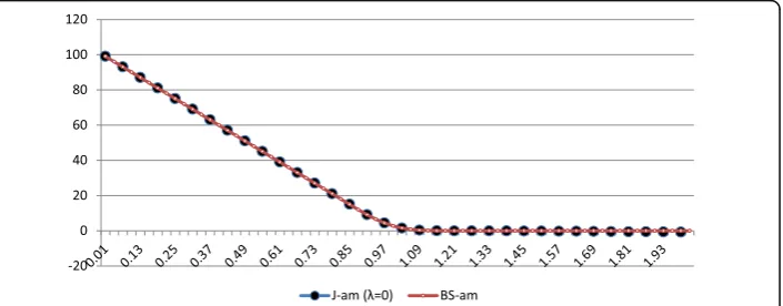
In Figs. 3 and 4, we plot the EEB curves of the BS-am and J-am (λ= 0) models and their differences. We notice that the EEB curves conform with the theoretical ones plotted in Fig. 1 for an American put. In Fig. 3, we notice that the EEB curves for both models, BS-am and J-am (λ= 0), approximately coincide since their difference is located in an interval [−0.04; 0.05]. Indeed, this error corre-sponds to the threshold authorized by iterative calculations. With a shorter time step Δω and with a longer computation time, this error can be reduced to an even lower level. For the two aforesaid models, we plot, in Fig. 5, both the Ameri-can and European option values as a function of their moneyness. Moreover, we plot, in Fig. 6, their EEP value ε as a function of moneyness. The curves in Figs. 5 and 6 are in accordance with the option theory and empirically confirm that the BS-am and J-am (λ= 0) models are the same. For all these computations, we Table 3Notation of functions = price difference between theJ-model and the Heston model. Notation of their minimas and maximas on the moneyness space

J-model vs BS model Heston-model vs BS model

Function Maxima Minima Function Maxima Minima

ΔJ−eur=PJ−eur−PBS−eur MJ−eur mJ−eur ΔHeston−eur=PHeston−eur−PBS−eur MHeston−eur mHeston−eur ΔJ−am=PJ−am−PBS−am MJ−am mJ−am ΔHeston−am=PHeston−am−PBS−am MHeston−am mHeston−am

εJ=PJ−am−PJ−eur MJ mJ εHeston=PHeston−am−PHeston−eur MHeston mHeston

ΔJ−ε=εJ−εBS MJ−ε mJ−ε ΔHeston−ε=εHeston−εBS MHeston−ε mHeston−ε

Fig. 3Comparison of the EEB given by the models BS-am andJ-am (λ= 0). Parameters values: K = 100,

consider a numerous time steps N equal to 50. The CPU time required by the J-model to compute the American option value is relatively longer than the one needed by the J-am model. This is because of the absence of a W-function library, allowing a quick computation, while we have a library for the standard normal law cumulative function. We should build such a library to ensure a quasi-instantaneous calculus of the American option value. In this paper, for further cal-culations and to perform them in a reasonable time, we take N= 10 instead of 50 or more. Although this choice slightly affects the accuracy of the results, it does not impact the results, curve profiles, and related conclusions.

American pricing model results based on theJ-am model

To examine the effects of the parametersλandθ on the EEB curve profile and Ameri-can option price related to J-am model, we plot, in Fig. 7, the EEB curves for various values ofλ: (λ= 1.6 orλ=−1.6) andθ: (θ=−3,θ= 0 orθ= 3). We notice that the effect of λ on the EEB profile is significant while the sensitivity to θ is very weak. The level of S_τ; as a limit value to early exercise of the option at a given time, de-creases with λ. For a given λ, the effect of θ (which ranges from −3 to +3) is not

Fig. 4Difference betweenJ-am (λ= 0) and BS-am models, in terms of EEB. Parameters values: K = 100,

τ=0.5,σ= 10%, r = 5%, Q = 5%,θ= 0.769 and N = 50

Fig. 5Comparison between BS-am andJ-am (λ= 0) models, in terms of European and American put prices.

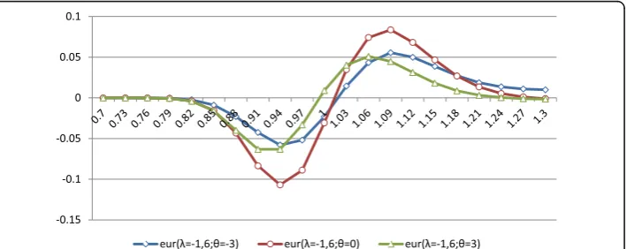
significant. For θ= 0, S_τ is maximum when λ is negative and minimum when λ is positive. The EEB curve related to the BS-am model is expected to be the same as the one related to J-am with λ= 0, as plotted in Figs. 3 and 4. In Fig. 8, we repre-sent the differences ΔJ−eur, ΔJ−am, and ΔJ−ε related to the parameters values (λ=

−1.6 and θ= 0). We notice that the curve ΔJ−eur is the same as the one elaborated

by Jerbi (2015). For a put, regardless of the moneyness, the difference ΔJ−ε=εJ −εBS is positive. With reference to the BS model, for negative values of λ, the

J-model overvalues the out-of-the-money European put and undervalues the in-the-money ones. With reference to the BS-am model, the J-am model overvalues the American puts when moneyness is less μ₁<1 or greater than μ₂>1; whereas it undervalues the American puts with moneyness located in the interval [μ₁; μ₂]. The differences: ΔJ−am=PJ−am−PBS−am and ΔJ−ε=εJ−εBS present positive

max-imums for a moneyness μ<μ₁<1<μ₂: Besides, for positive values of λ, the pro-file of the curve ΔJ−am is nearly the same as the one of ΔJ−eur. The differenceΔJ−ε =εJ−εBS is positive for in-the-money puts, whereas it is negative for out-of-the-money

puts. In Figs. 9 and 10, for λ=−1.6 and λ= 1.6, respectively, we plot ΔJ−eur for

Fig. 6Comparison between BS-am andJ-am (λ= 0) models, in terms of American early exercise put price.

Parameters values: K = 100,τ=0.5,σ= 10%, r = 5%, Q = 5%,θ= 0.769 and N = 50

Fig. 7EEB related to the BS-am andJ-am for various values of the parametersλandθ. Parameters values:

various values of θ. We do the same for the differences ΔJ−am (Figs. 11 and 12)

and ΔJ−ε (Figs. 13 and 14).

Regarding ΔJ−eur, we confirm the results found by Jerbi [1]. Regarding the value

of λ, the maximum and the minimum of the difference ΔJ−eur are related to θ= 0.

These extreme values are close to those related to θ= 3 and θ=−3. Regarding ΔJ −am, for positive values of λ, the curve profile function of the moneyness is quite

similar to the one related to ΔJ−eur. For negative values of λ, the curve profile is

almost the same as the corresponding ΔJ−eur, with the only difference that it

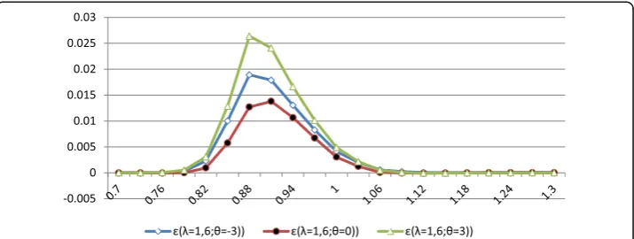
pre-sents a positive maximum located in the moneyness interval [0.85; 0.9]. This max-imum coincides with the maxmax-imum of ΔJ−ε, as indicated in Fig. 13. In this figure, we see that the effect of θ on ΔJ−ε is negligible when λ is negative. However, when λ is positive, the εJ value is sensitive to changes in the parameter θ. This is

because the εJ value increases with the absolute value of this parameter, with a

maximum value corresponding to the same moneyness.

Equivalence condition between theJ-am model and Heston-am one

The comparison between theJ-am and Heston-am models is performed with reference to the BS and BS-am models. Hence, we examine the skewness and kurtosis effects on

Fig. 8Comparison:ΔJ‐eur,ΔJ‐amandΔJ‐ε(λ=−1.6 andθ= 0). Parameters values: K = 100,τ=0.5,σ= 10%, r = 5%, Q = 5%

American option pricing related to the two aforesaid models. As indicated by Jerbi (2015), we compare the J-model results with those of Heston (1993) with regard to European option pricing. We find that these two models give the same shapes of the curves ΔJ−eur(S/E) for various values of the parameter ρ(λ). To empirically

compare the J-model and Heston one, we consider the same volatility parameter values used by Heston (1993) (v= 0.01; σ= 0.1; κ= 2; φ= 0.01 and ρ= 0.5 and −0.5) and we plot the respective curves of option difference value with the one of the BS model. To determine the values of parameters λ* and θ* regarding the J-model (see Jerbi (2015)) and those corresponding to the aforesaid Heston parameters, we use two approaches. In the first approach, equivalence is based on the dynamics of the underlying asset, in the second approach, the equivalence is based on the European option price J-formula and Heston’s model. As indicated by Jerbi (2015), we find that λ* = 0.84 and θ* = 0.769, with an estimation error equal to 6,782 E-07). In the second approach, to determine λ* and θ* corresponding to the optimal equivalence, we minimize the gap between the J-model and Heston’s model. For a given ρ, we estimate the values of λ* * and θ* * by considering the minimum of the difference between the two model prices:

λ_;θ

ð Þ ¼Argmin

λ;θ fJeurðλ;θÞ−Hestoneurðκ;ϕ;η;ρÞg 2

Fig. 10Comparison:ΔJ‐eurwith (λ= +1.6 andθ=−3,θ= 0 orθ= 3). Parameters values: K = 100,τ=0.5, σ= 10%, r = 5%, Q = 5%

We notice that using the second equivalence approach based on the volatility param-eters used by Heston (1993) (v; κ; φ; ηand ρ), for ρ= 0.5 andρ=−0.5, the difference ΔHeston−euris almost at its minimum for λ* *= 1.6 and λ* * =−1.6, respectively. Unlike

the bi-dimensional Heston model, which is based on Fourier inversion, the J-model has the advantage of being a uni-dimensional model using a simple computational technique. We can say that “the use of only one state variable following the J-process” is equivalent to the use of two correlated state variables following the Wiener process. Here, we extend the equivalence to American options. If we con-sider the previous values of λ= 1.6 and λ=−1.6 for the J-am model and ρ= 0.5 and ρ=−0.5 for the Heston-am model, in plotting the respective EEB curves in Fig. 15, we find that the equivalence encountered in the study by Jerbi (2015), for the European options, remains true for the American options. These values of λ are only approximate. Hence, they can be adjusted more accurately to fit the Hes-ton model. In Fig. 12, we notice that regardless of the model chosen, the profile of the EEB curves fits the theory. For a given time, during the life of option, the early exercise is optimal for S*. This level S* decreases with λ for the J-am model and with ρ for the Heston-am model. Moreover, we notice that the parameter value equivalence studied by Jerbi (2015) remains valid for the American option, since we have the correspondence (λ= 1.6 and λ=−1.6) in the J-am model to (ρ= 0.5 and ρ=−0.5) that in Heston’s model. The EEB curve related to BS-am is consid-ered to be the same as the J-am one with λ= 0.

Fig. 12Comparison:ΔJ‐amwith (λ= +1.6 andθ=−3,θ= 0 orθ= 3). Parameters values: K = 100,τ=0.5, σ= 10%, r = 5%, Q = 5%

Comparison betweenJ-am model and Heston-am one in terms of the volatility effect when the equivalence condition is satisfied

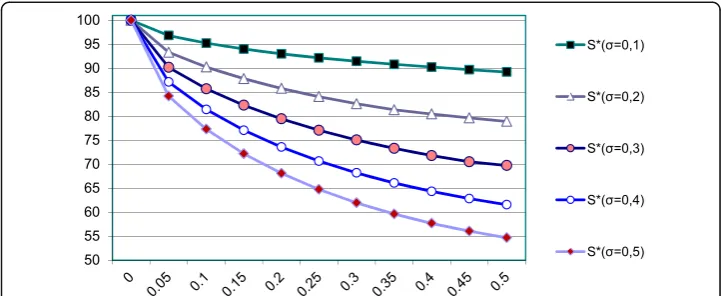
Since the option value is sensitive to the volatility change, we must examine the ef-fect of such a variable on the option price for various values ranging from 10 to 50%, with a rising gap of 10%. We begin by examining the EEB curves of the J-am model with parameters λ=−1.6 and θ* = 0.769, plotted in Fig. 16: we compare this with the Heston model related to the parameters (κ= 2; φ= 0.01 and ρ=−0.5) with a variance v= 0.01, plotted in Fig. 17. We notice that although the curve profiles are quite similar, we find that only for σ= 10% (i.e. v= 0.01), the J-am EEB exactly coincides with the Heston one. This is quite normal because for ρ=−0.5, the re-lated value λ=−1.6 is based on the dynamics of the CIR used by Heston for a value of v= 0.01. This means that for each value of v, we must compute the new related value of λ. Since we consider the same value of λ regardless of the value of v, the equivalence between the two models, in terms of EEB, is valid only for v= 0.01. The comparison between the J-model and Heston’s model enables us to examine the skewness and kurtosis effects on the European or American put.

Fig. 14Comparison:ΔJ‐εwith (λ= +1.6 andθ). Parameters values: K = 100,τ=0.5,σ= 10%, r = 5% and Q = 5%

Fig. 15Comparison of the EEB related to the BS-am andJ-am and Hesston-am models, Parameters values:

These effects are induced by the stochastic volatility effects in the Heston model and the J-process effects in the J-model. For λ=−1.6, we plot ΔJ−am in Fig. 18:

for the equivalent value ρ=−0.5, we plot ΔHeston−am in Fig. 19. We notice that,

for negative values of λ and ρ, these two differences are negative and decrease with volatility. The value −1.6 of λ was computed for ρ=−0.5 and for a variance ν= 0.01. If we adapt the estimation of the parameter λ to the variance value, the ΔHeston−am curves should be the same as the ΔJ−am ones plotted in Fig. 18. For

the reason previously evoked, this is only the case for ν= 0.01. When λ and ρ are positive, ΔJ−am and ΔHeston−am are positive for in-the-money puts and negative

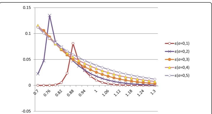
for out-of-the-money puts. Hence, compared with the BS-am model, for negative values of λ or ρ, (Figs. 18 and 19), the J-am and Heston-am models undervalue the American in-the-money puts and overvalue the out-of-the-money ones and vice versa. These curves are approximately the same for (λ=−1.6 and ρ=−0.5) and for (λ= 1.6 and ρ= 0.5), when the volatility equals 10%. Besides, the curves related to εJ and εHeston are similar, as shown in Figs. 20 and 21. The maximum

of the premium increases with the volatility level and corresponds to a lower moneyness.

Fig. 16EEB related toJ-am with parameters values: K = 100,τ=0.5,σ= 10%, r = 5%, Q = 5%,J-am (λ=−1.6 withθ= 0.769)

Fig. 17EEB related to Heston-am models, with parameters values: K = 100,τ=0.5,σ= 10%, r = 5%, Q = 5%,

Comparison betweenJ-am and Heston-am models in terms of the effect of the time to maturity

Here, we examine the effect of the time to maturity (ranging from 0.1 to 1 year) on the American option price. For the European options, the problem is examined in the study by Jerbi (2015) and extended here to the American options. First, the EEB does not depend on the time to maturity, which means that for the values considered, we have the same curve support limited in time by the aforesaid values. We plot, in Fig. 22, the EEB related to the J-am model for various values of λ as well as for the ones related to the Heston-am model for various values of the correlation factor ρ. The volatility is set equal to 10% for all the curves consid-ered. The EEB (λ= 1.6) coincides with the one related to (ρ= 0.5), while the EEB (λ=−1.6) coincides with the one related to (ρ=−0.5). The EEB corresponding to the BS-am model is close to the Heston-am related to (ρ= 0). The precision of the price mainly depends on the accuracy of the determination of the EEB. Here, we have a tradeoff between the accuracy and the CPU time convergence. For a given time step, the EEB boundary does not depend on τ(Fig. 23).

Fig. 18ΔJ‐amas a function of moneyness, for various values of the Volatility, with parameters values: K = 100,τ=0.5,σ= 10%, r = 5%, Q = 5%, (λ=−1.6,θ= 0.769)

Unlike with the European puts, in the case of in-the-money American puts, when λ and ρ are negative, there is a small moneyness interval where the models J-am or Heston-am overvalue the option price compared with the BS-am model (Figs. 24 and 25). This interval does not exist for positive values of the parameters λ and ρ (Figs. 26 and 27). In all the other cases, the results for the American options are the same as those of the European ones encountered in the study by Jerbi (2015). Either for J-am model or the Heston-am one, the greater the time to maturity, the greater the difference with BS-am. Thus, we consider the EEP εJ and εHeston as functions of moneyness for the various values

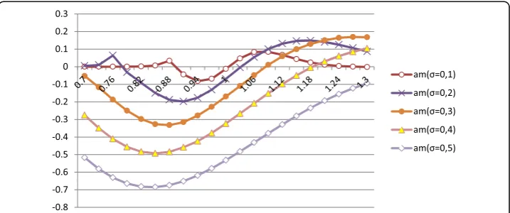
of the option maturity. Indeed, we examine the skewness and kurtosis effects on this option price. We notice that the two studied models give the same results for λ = −1.6 and ρ = −0.5 (Figs. 28 and 29), with positive values regardless of the moneyness. For each time to maturity τ, εJ presents a maximum ε x_τ for a

moneyness x_τ less than the unity. The value of x_τ decreases with τ, while ε x_τ

Fig. 20ΔJ‐εas a function of moneyness for various values of volatility, with parameters values: K = 100,

τ=0.5,σ= 10%, r = 5%, Q = 5%, and (λ=−1.6 andθ= 0.769)

increases. In case λ= 1.6 and ρ= 0.5, the J-am and Heston-am models give the same results. For τ less than almost τ* = 0.6, the skewness and kurtosis induce positive values in the EEP, while for τ greater than τ*, we find a negative effect for a moneyness ranging from x_1;τ and a positive effect for a moneyness greater than x_1;τ (Fig. 30).

Finally, we can say that the comparison between the models is based on the ef-fect of the stochastic volatility of the American option pricing. We have proved that the J-am is an extension of the model BS-am, as we did with the J-model and BS models. Furthermore, we conclude that the J-am model gives the same results as the Heston-am one in considering equivalent parameters ensuring equivalent ef-fects of skewness and kurtosis. The equivalence between the two models can be improved with an accurate estimation of parameters λ and θ for given values of the volatility dynamics parameters considered in the Heston model.

Fig. 22Comparison between the EEB related to the BS-am andJ-am and Heston- am models, Parameters

values: K = 100,τ=1,σ= 10%, r = 5%, Q = 5%,J-am (λ= 1.6 and−1.6 withθ= 0.769). Heston-am (v = 0.01; κ= 2;φ= 0.01 andρ= 0.5; 0 and−0.5)

Fig. 23ΔJ‐amas a function of moneyness, for various values of time to maturity, Parameters values:

Comparison between theJ-am and the Heston-am models in terms of CPU time

For the three models, BS-am, Heston-am, and J-am, the CPU time required for comput-ing the American put price is indicated in Table 4. The first part of this time CPU1 deter-mines the EEB through 10 steps of the residual option lifetime. Once the 10 EEB points are computed, we calculate the American option value related to 21 levels of moneyness. This calculation requires the second part of time CPU2 such that CPU = CPU1 + CPU2. The BS-am requires a relatively short CPU time, either for determining the EEB or for computing the American put value. TheJ-am model requires a long time to perform the same tasks. This is due to the fact that the basic functionWis numerically computed as an integral, which is time consuming. The Heston model, based on the Fourier inversion, requires a significantly lower CPU time than the one needed by theJ-am model to com-pute the American put value. To drastically improve the speed of theJ-am model conver-gence, we should build a library of the function W, similar to the one corresponding to the standard normal cumulative function. Hence, the CPU time required by the J-am model will be the same as the one required by BS-am model and significantly better than the one required by Heston-am model. Since theJ-am model considers the skewness and kurtosis effects, which is not the case with the BS-am model, theJ-am represents the best

Fig. 24ΔHeston‐amas a function of moneyness, for various values of time to maturity. Parameters values:

K = 100,τ=0.5, r = 5%, Q = 5%, (v = 0.01,κ= 2,φ= 0.01 andρ=−0.5)

Fig. 25ΔJ‐amas a function of moneyness, for various values of time to maturity, Parameters values:

compromise between accuracy that conforms to the financial market reality and CPU time consumption.

Improvements of theJ-am model

The valuation of the American option accuracy highly depends on the accuracy of the de-termination of the EEB. The errors are cumulated along the residual lifetime of the option. Hence, approaching the border with a high polynomial degree can preserve the accuracy of the calculation of this boundary. Hence, we can maintain the accuracy of the American option value. Simultaneously, we significantly reduce the required CPU time to compute the American option value. To do this, for the three models and reduce the computation complexity of the American option price, we model the EEB as a polynomial of a degree 10 (as we used 10 steps to determine the EEB) as follows:

Sð_τ−ωiÞ¼

X

k¼0 k¼10

αkðτ−ωiÞk

where 0≤ωi≤τand is an integer : 0≤i≤10.

If we denote by ω1=τ>ω2>ω3>... >ω9>ω10> 0 the values related to ωi (with

0≤i≤10) and by Sðτ−ωiÞ for the corresponding 10 limit values, which are computed

Fig. 26_ΔHeston‐amas a function of moneyness, for various values of time to maturity. Parameters values:

K = 100,_τ=0.5, r = 5%, Q = 5% with (v = 0.01,_κ= 2,_φ= 0.01 and_ρ= 0.5)

Fig. 27ΔJ‐εas a function of moneyness for various values of time to maturity, Parameters values: K = 100,

with the aforesaid algorithm, we can determine the coefficients αk (with 0≤k≤10) of

the polynomials through a Cramer system of degree 10. The coefficients related to Figs. 16 (J-am model) and 17 (Heston model) are given in Table 5. These coefficients are computed numerically. Therefore, we can express them as functions of the Ameri-can option inputs to analytically compute the AmeriAmeri-can option value.

Conclusion

In this study, we have elaborated a new uni-dimensional modelJ-am for pricing American options, which is based on the J-model developed by Jerbi (2015). We have shown that this model is an extension of the American model BS-am based on the BS model. As indi-cated by Jerbi (2015), we have examined the equivalence between theJ-model and Heston one. Here, we have extended the study of this equivalence to American options. The pa-rameters of theJ-process ensuring this equivalence were determined as the values minim-izing the squared errors between the J-process and CIR process used in the study by Heston (1993). We notice that these parameters can also be determined as the values minimizing the error between theJ-am formula and Heston-am one. This study aimed to

Fig. 28ΔHeston‐εas a function of moneyness, for various values of time to maturity, Parameters values:

K = 100,τ=0.5, r = 5%, Q = 5%, (v = 0.01,κ= 2,φ= 0.01 andρ=−0.5)

Fig. 29ΔJ‐εas a function of moneyness for various values of time to maturity, with parameters values:

compare a confirmed model, the Heston’s, which is bidimensional, with an equiva-lent unidimensional model J-am. Assuming that we use the equivalent parameters λ* and θ*, we can say that our results regarding the J-am are totally in accordance with those of Heston’s in terms of EEB and American option pricing. The EEB and the American option price profiles generated by all the chosen models fully con-form with the options theory. We have examined the similarity between the effect of λ* and ρ and the one between θ* and (κ; φ; η; v). We can say that the skewness and kurtosis effects induced by the stochastic aspect of the volatility in the bidi-mensional model of Heston, are equivalent to the ones generated by the extension of the Wiener process to the J-process. This was our conclusion, as indicated by Jerbi (2015), and we extended this conclusion to the American options. For a fu-ture work, we plan to examine the dynamic risk management related to an Ameri-can option portfolio based on this model. We Ameri-can also use this model to solve financial or economic problems based on American options, such as the decision optimization in an area characterized by innovation and technical progress. TheJ-am, as a uni-dimensional model, is expected to fit the reality of the financial market with a better compromise between accuracy and CPU time than the Heston-am model. The computation, based on the cumulative function F of the J-law, is easier than the one based on the Fourier inversion method used by Heston. A library for the function F must be constructed to ensure the optimality of the J-am model in terms of accuracy and time consumption. Moreover, the modeling of the EEB based on the polynomial approach can be carried out to significantly improve the CPU time needed to compute the American option value for a given accuracy. Fi-nally, the results generated by the J-am model must be compared with those gen-erated by simulations based on Malliavin calculus and using the J-process (see Jerbi and Kharrat (2014)).

Fig. 30_ΔHeston‐εas a function of moneyness, for various values of time to maturity, with parameters

values: K = 100,_τ=0.5, r = 5%, Q = 5%, Heston-am (v = 0.01,_κ= 2,_φ= 0.01 and_ρ= 0.5)

Table 4The CPU Time required at each stage for determining the American option

Time CPU (in second) BS-am Heston-am J-am

CPU1: OEB determination (10 points) 1 430 5584

Table 5The OEB approximate polynomial coefficients for theJ-am (λ=−1.6,θ= 0.767) and Heston (v = 0.01,κ= 2,φ= 0.01 andρ=−0.5) models, for various values of the volatility

OEB S*(σ= 0,1) S*(σ= 0,2) S*(σ= 0,3) S*(σ= 0,4) S*(σ= 0,5)

J-am Heston-am J-am Heston-am J-am Heston-am J-am Heston-am J-am Heston-am

α0 100 100 100 100 100 100 100 100 100 100

α1 −88,7 −182,8 −251,4 −242,6 −357,3 −572,9 −469,3 −396,1 −577,6 −684,3

α2 454,0 3781,6 4223,9 2148,9 5524,5 13660,0 7252,0 −1198,9 8864,3 9248,4

α3 4719,5 −47754,5 −55634,7 −4162,3 −66543,0 −219163,6 −86741,4 119100,6 −104209,1 −86821,5

α4 −113190,0 358207,8 481249,7 −129020,2 526397,3 2134038,5 682209,7 −1781952,0 805895,7 532016,2

α5 957015,7 −1687800,5 −2768878,8 1470870,0 −2764903,7 −13022337,6 −3559002,7 13594552,2 −4135421,6 −2260576,2

α6 −4473462,2 5132416,9 10680702,7 −7709733,4 9728193,1 51049511,1 12413443,5 −61391738,5 14195574,1 7125696,7

α7 12559747,8 −10044517,7 −27258807,6 23187361,5 −22664547,0 −128519111,3 −28605887,8 170587764,1 −32220275,1 −16790157,4

α8 −21096551,5 12180376,5 44059429,4 −40996252,7 33535228,2 200843071,0 41770962,5 −286783820,3 46384859,5 27432124,8

α9 19564855,4 −8286347,9 −40740040,3 39687366,2 −28523653,2 −177308022,0 −34985276,1 267836101,2 −38341325,4 −26780575,1

α10 −7712384,0 2399990,3 16372793,2 −16255502,5 10614375,1 67563228,8 12792706,6 −106721471,3 13851225,0 11487040,7

lInnovation

(2016) 2:21

Page

24

of

Appendix

EEP formula based on theJ-model

For an American put, the EEP is: ε¼

Z

0 T−t

e−rωZ Sðτ−ωÞ

0

rK−Qsω

ð ÞhSð Þsω dsωdω, where

hS(sω) is the probability density function of the underlying asset priceSωat a time t ran-ging from 0 to the option time to maturity. The underlying asset, distributing dividends

at a rate Q, follows a J-process defined by the following SDE: dSt_St ¼ðr−QÞdtþσpffiffiffiffiffidtUt, where Ut¼Wt_σ−_WEW with W following the J-Law (see Jerbi (2015), with expected value

EW=E(Wt) and standard deviationσW ¼

ffiffiffiffiffiffiffiffiffiffiffiffiffiffiffi

V Wð tÞ

p

.

Applying the Ito’s lemma and replacingUtby its expression, and integrating from 0

toω, we have:Ln Sω

St ¼ r−Q−σ 2 2

ω− σ σWEW

ffiffiffiffi

ω

p

þWω_σσ_Wpffiffiffiffiω. If we put:

a¼ r−Q−σ 2

2

ω−_σWσ EW

ffiffiffiffi

ω

p

b¼ σ σW ffiffiffiffi ω p 8 > < >

: we can write

Sω¼SteaþbWω

Wω¼1

b Ln Sω St −a 8 < :

As S_ω is a strictly monotonous function ofW_ω, we can writeh(s_ω)ds_ω=g(w_ω)dw_ω. If

we putHð Þ ¼ω

Z Sðτ−ωÞ

0

rK−Qsω

ð ÞhSð Þsω dsω, the premium is thenε¼ Z

0 T−t

e−rω_{Hð Þω dω.}

In replacing s_ω by its expression as a function of w_ω, we get: Hð Þ ¼ω

Z

−∞

w_ðτ−ωÞ

rK−QSteaþbwω

g wð Þω dwω.

H(ω) can be written as the difference :H(ω) =H1(ω)−H2(ω) with :

H1ð Þ ¼ω rK

Z

−∞

w_ðτ−ωÞ

f wð Þω dwω

H2ð Þ ¼ω QSt

Z

−∞

w_ðτ−ωÞ

eaþbwω e

−1 2w

2

Jerðλ;θÞpffiffiffiffiffiffi2πNðλwωþθÞdwω

8 > > > < > > > :

If we name F the cumulative function of theJ-law, we have:

H1ð Þ ¼ω rK F wð_τ−ωÞ;λ;θ

H2ð Þ ¼ω QSte aþb

2

2

Z

−∞

w_ðτ−ωÞ e

−1 2ðwω−bÞ

2

Jerðλ;θÞp2ffiffiffiffiffiffiπNðλwωþθÞdwω

8 > > > < > > > :

We putZω=Wω−b,Zωfollows theJ-law such as:Zω→J(λ,λb+θ). Hence, we have: H1ð Þ ¼ω rK F wð_τ−ωÞ;λ;θ

H2ð Þ ¼ω QSte aþb

2

2F z_ðτ−ωÞ;λ;λbþθ

8 > > < > > :

withz_ðτ−ωÞ¼w_ðτ−ωÞ−b

If we callΦ¼−σ2₂ω 1−_σ12 W

−σ_σp_WffiffiffiωEW;we haveaþb 2

2 ¼rω−QωþΦ. Hence,H(ω) can be written as follows:Hð Þ ¼ω rK F w_ðτ−ωÞ;λ;θ

−QSterω−QωþΦF zð_τ−ωÞ;λ;λbþθ

.

We deduce the expression of the EEP:ε¼

Z

0T−t

Gð Þω dω

withGð Þ ¼ω rK e−rω_{F w}

τ−ω

ð Þ;λ;θ

−QSte−QωþΦF zð_τ−ωÞ;λ;λbþθ

wherew_ðτ−ωÞ¼Ln Sw St − r−Q−σ

2 2

ωþσ σWEW

ffiffiffi ω p σ σW ffiffiffi ω

p _andz

τ−ω

ð Þ¼wðτ−ωÞ−b.

We notice that:

zðτ−ωÞ¼−σWd1;ωþEW

wðτ−ωÞ¼−σWd2;ωþEW

(

withd1;ω¼Ln

St Sw

ð Þþ r−Qþσ22

ω

σpffiffiffiω etd2;ω¼d1;ω−σpffiffiffiffiω

If we setλ= 0, we get the EEP formula for an American put related to BS-am model:

ε¼

Z τ

0

rK e−rωN −d2;_ω

−QSte−QωN −d1;ω

dω

Acknowledgement

I have achieved all the work by myself and I have no acknowledgement to mention in the Acknowledgement section. Competing interest

The author declares that he has no competing interests. Received: 22 February 2016 Accepted: 28 November 2016

References

Black F, Scholes M (1973) The pricing of options and corporate Liabilities. J Polit Econ 81(May-June):637–654 Brennan M, Schwartz E (1977) The valuation of American put options. J Financ 32:449–462

Broadie M, Glasserman P (1997) Pricing American-style securities using simulation. J Econ Dyn Control 21:1323–1352 Carr P, Wu L (2004) Time-changed levy processes and option pricing. J Financ Econ 17(1):113–141

Clarke N, Parrott K (1999) Multigrid for American option pricing with stochastic volatility. Applied Mathematical Finance 6:177–195

Detemple J, Rindisbacher M (2005) Closed-form solutions for optimal portfolio selection with stochastic interest rates. Math Financ 15:539–568

Detemple J, Tian W (2002) The valuation of American options for a class of diffusion processes. Manag Sci 48:917–937 Garman MB (1976) A general theory of asset valuation under diffusion state processes, research program in finance,

Working papers 50, University of California at Berkeley

Haugh M, Kogan L (2004) Pricing American options: a duality approach. Operation Research 52:258–270 Heston SL (1993) Closed form solution for options with stochastic volatility with application to bonds and currency

options. Rev Financ Stud 6(2):327–343

Huang J, Subrahmanyam M, Yu G (1996) Pricing and hedging American options: a recursive integration method. Rev Financ Stud 9:277–300

Hull J, White A (1987) The pricing of options on assets with stochastic volatilities. J Financ 42(2):281–300 Ikonen S, Toivanen J (2007) Efficient numerical methods for pricing American options under stochastic volatility.

Numerical Methods for Partial Differential Equations 24:104–126

Jerbi Y (2011) New statistical law-namedJ-law and its features. Far East Journal of Applied Mathematics 50(1):41–56 Jerbi Y (2015) A New closed form solution as an extension of the Black & Scholes formula allowing smile curve

plotting. Quantitative Finance 15(12):2041–2052

Jerbi Y, Kharrat M (2014) Conditional expectation determination based on theJ-process using Malliavin calculus applied to pricing American options. J Stat Comput Simul 84(11):1–9

Ju N (1998) Pricing an American Option by approximating its early exercise boundary as a multi piece exponential function. Rev Financ Stud 11(3):627–646

Kim IJ (1990) The analytical valuation of American options. Rev Financ Stud 3:547–572 Kwok Y-K (1998) Mathematical model of financial derivatives, Springer

Longstaff F, Schwartz E (2001) Valuing American options by simulation: a simple least-squares approach. Rev Financ Stud 14:113–147

Rogers L (2002) Monte Carlo valuation of American options. Math Financ 12:271–286

Stein EM, Stein JC (1991) Stock price distributions with stochastic volatility: an analytic approach. Rev Financ Stud 4(4): 727–752

Sullivan M (2000) Valuing American put options using Gaussian quadrature. Rev Financ Stud 13:75–94