A Two-Step Method for Damage Identification and Quantification in Large Trusses via Wavelet Transform and Optimization Algorithm

DOI: 10.22075/JRCE.2017.11678.1197

Journal homepage: http://civiljournal.semnan.ac.ir/

A Two-Step Method for Damage Identification and

Quantification

in

Large

Trusses

via

Wavelet

Transform and Optimization Algorithm

B. Mirzaei1, K. Nasrollahi1, S.M.M. Yousefbeik1, G. Ghodrati Amiri2* and A. Zare

Hosseinzadeh2

1. School of Civil Engineering, Iran University of Science and Technology, Tehran, Iran

2. Center of Excellence for Fundamental Studies in Structural Engineering, School of Civil Engineering, Iran University of Science and Technology, P.O. Box 16765-163, Tehran, Iran

* Corresponding author: [email protected]

ARTICLE INFO ABSTRACT

Article history:

Received: 18 June 2017 Accepted: 31 October 2017

This paper suggests a two-step approach for damage prognosis in long trusses in which the first step deals with locating probable damages by wavelet transform (WT) and static deflection derived from modal data with the intention of declining the subsequent inverse problem variables. And in the second step, optimization based model updating method applying Artificial Bee Colony (ABC) algorithm will be employed to quantify the predicted damages within an inverse problem. Interestingly, it is indicated that the two-step method greatly aids in declining the number of variables of the model updating process resulting in more precise results and far less computational effort. Moreover, the method is found considerably effective especially for damage prognosis of large trusses. In this regard, two numerical examples including noisy data are contemplated to assess the efficacy of the method for real practical problems. Furthermore, the validity of the second step results is investigated applying other optimizers namely Invasive Weed Optimization (IWO) and Particle Swarm Optimization (PSO).

Keywords:

Structural Health Monitoring, Damage Detection,

Wavelet Transform, Model Updating, Large Trusses.

1. Introduction

During the serviceability, a structure experiences a variety of damages which bring either partial or significant adverse effects on its performance. Consequently, Structural Health Monitoring (SHM)

quantified as well. A rather thorough review on new and traditional damage detection methods is discussed in [1, 2]. As a result to high capability of wavelet transform, henceforth referred to as WT, in revealing singular points in a given signal, either stationary or non-stationary, it has been extensively employed in damage detection literature. One of the first scholars utilizing WT for damage detection purposes is [3] in which not only have the authors authenticated that damages will emerge as singular points in the deflection curve, however they have carried out experiments to validate their method as well. This vibrational technique and its applications are comprehensively reviewed in [4]. In most WT literature, researchers utilized WT only to pinpoint damage locations and the damage severities were not quantified by this method. An illustration of this can be found in [5] where WT is applied for locating damage in truss structures. An identical approach is adapted in [6] for spotting impairments in plate structures. A new damage index based on wavelet residual force is introduced in [7] in order to compute where damages took place in shear, plane frames in time-domain. Moreover, a complex mother wavelet is utilized in [8] for multiple damage detection in Euler beams. On that account, one of the major demerits of WT is its incapability in directly identifying damage severities especially in the displacement-domain. In order to address this issue, researchers have put forth a number of indirect methods for finding damage severities. For instance, [9] discrete wavelet transform (DWT) is applied to localize structural defects, and a statistical approach is suggested to predict the extent of defects based on wavelet coefficients. Moreover, in a number of recent studies, two-step approaches are opted to overcome

frequencies and mode shapes is investigated in [15] where Charged System Search (CSS) algorithm and Enhance Charged System Search (ECSS) are utilized to search for global optimum. In [16], the problem of damage detection using modal data is solved via CSS optimization algorithm and their proposed method is also validated by using three numerical examples. The problem of damage detection is solved applying frequencies and mode shapes of structures via the model updating technique using Magnetic Charged System Search (MCSS) and PSO in [17]. By utilizing natural frequencies and mode shapes to generate an Objective Function (O.F), a damage detection method based on model updating is proposed in [18] where the optimization problem is solved by continuous Ant Colony algorithm. The ABC optimization algorithm is chosen to be the optimizer to solve the damage detection problem in [19, 20] in which the authors develop an O.F by a combination of natural frequencies and modal shapes of the structure. In [21] the authors detect damages of truss structures by applying simplified Dolphin Echolocation (DE) algorithm. The O.F in the mentioned paper is formed based on natural frequencies and mode shapes of the structure. Despite the fact that model updating is regarded as one of the most effective methods of damage localization and quantification, it has one major drawback. When the number of variables considerably increases in the inverse problem, it either diverges or converges to wrong results. To tackle this problem, generally, two-step approaches are employed. To provide an illustration, it can be referred to [22] in which a two-step method is presented for damage localization and quantification in linear-shaped structures via Grey System Theory (GST) and an

optimization-based procedure. Another example of two-step methods can be seen in [23] in which the authors proposed a two-step technique applying residual force vector and model updating method in which damaged elements are located during the first step and the severity of damage in the located elements are determined using a sensitivity-based model updating method. The method is tested on different examples. However, structures with large number of elements are not tested.

In this paper, in order that the merits of both Wavelet transform and model updating can be simultaneously employed and their drawbacks can also be offset, a two-step method is proposed which requires data from damaged structure and stiffness matrix of undamaged structure only, based on which both location and severity of damage will be measured. In the first step, damaged areas are predicted by exerting continuous wavelet transform (CWT). In the next step by recruiting model updating method, damage severities in nominated elements are quantified. It is noteworthy to mention that the most considerable merit of the presented method in comparison with other multistep approaches is its effectiveness in analyzing large structures with modest amount of data.

2. Theoretical Background

2.1. Wavelet Transform

definition of CWT is provided in equation. (1). More details are presented in [24-26].

f

1

CWT Coeff ,  (x) dx

 



x - b

= W (a b) = f . ( ) a

a (1)

where ψ x

 

is a mother wavelet function with zero mean value for which satisfying two crucial conditions is imperative [24]. In equation. (1),a> 0, and a and b are both real numbers. The variables a and b represent the mother wavelet width (scale) and translation along length axis, respectively. 

 

x is the complex conjugate of ψ x , andW (a b)f , is the wavelet coefficient matrix.

2.1.1. Border Distortion Effect

An issue which limits the application of WT is associated with signal borders [27]. As a result to this effect, singular behavior is observed at signal borders in wavelet coefficient graph (which are the location of end supports in some structures), which might even lead such locations to being regarded as damaged mistakenly. Therefore in order to cope with this so called edge effect or border distortion, researchers have recommended the signal extension technique with the intention of expelling edge effect out of the original signal [27-29]. The signal extension technique suggests extending the signal on both ends and then cutting again the extended parts after CWT is applied. In this way, the singularities occurred in both ends of the signal will be eliminated.

2.2. Objective Function

A desirable O.F should consist of structural updating parameters sufficiently sensitive to structural damage as well as being insensitive to other disruptive parameters such as additive noise. Assuming differential equation of motion for a linear structure as equation. (2):

Mx + Kx = 0 (2)

Free vibration equation of the structure with

dof

N degrees of freedom could be derived as equation. (3):

j j

λ = ,

(K - M)Φ 0

dof

j = 1, 2, 3,..., N (3)

In the aforementioned equation, K and M represent global mass and global stiffness matrices, respectively. If the situation of the damaged structure is substituted into the above equation, equation. (4) yields:

j

d d d

j

λ ,

(K - M)Φ = 0

dof

j = 1, 2, 3,..., N (4)

Equations. (3), (4) are the first and foremost mathematical basis for generating a new O.F. In the above equation, _Kd

is the global stiffness matrix for the damaged structure, M is the global mass matrix considered to be immutable in damaged circumstance, and d

j λ

represents the square of natural frequencies then Φj are mode shapes corresponding to j

th

mode of damaged structure. The number of natural modes is stated as “Ndof ”.

 d

M M (5)

According to equation. (4), the following equation is resulted:

d d d

i λi i i = 1, 2, 3,…, N dof

d

KΦ = MΦ     ₍₆₎

By multiplying both sides of the equality by

 

d T

i

Φ and performing mass normalization, the following equation is obtained, where d

K

is the global stiffness matrix for damaged state derived from modal data:

   

-T -1

d d d

d

Φ is eigenvector for the damaged structure, and Λ is representative of a diagonal matrix possessing eigenvalue components of the damaged structure:

dof

d d 2

1

d 2

d 1

N

d

2 n

(ω ) 0

0 (ω )

ω < ω <…< ω

 

 

  

 

 

Λ (8)

F is the flexibility matrix, which is the inverse of stiffness matrix, and could be written as below for the damaged state:

 

-1 T

d d d d

F = Φ   Λ Φ (9)

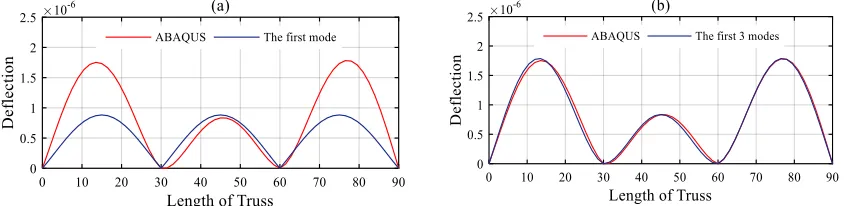
As it is vividly observed in equation. (9), there is an inverse correlation between flexibility matrix and eigenvalue matrix; that is, as the number of modes grow, higher mode shapes play a lesser role in constructing the flexibility matrix. More precisely, it could be determined that initial modes of the structure play more pivotal roles in shaping the flexibility matrix. Thus, it is reasonable to capture the first m modes in order to estimate the flexibility matrix.Morover, from practical

perspective, it is not feasible to capture all of the structural modes. Therefore, only the first, the first three and the first five modes are employed in the present study for damage detection purposes. Assuming that the first m modes are contemplated for forming the flexibility matrix, static deflection estimated by the first m modes could be obtained by the following equation:

m. I

U = F f ₍₁₀₎

In which:





T

I 1,1 , ,1 1×m

f (11)

The former equation delineates that static deflection could be derived by modal-based flexibility matrix with unit loads exerted on the entire degrees of freedom [30]. A comparison between static deflections resulted from static analysis via ABAQUS software and modal analysis applying a limited number of modes in MATLAB environment is provided in Figure 1, where a negligible difference can be observed.

Fig. 1. Comparison between static deflections resulted from static analysis with ABAQUS and

modal analysis in MATLAB for model 1 for down path and estimation with (a) the first mode, (b) the first three modes.

If damaged state is substituted into equation. (10):

d d m.I

U = F f ₍₁₂₎

To suggest the O.F, firstly let’s assume that displacement components UI are defined as:

 

 

 

T

I  m 1,1 , m 2,1 , … , m n,1

U = U U U (13)

 

 

 

d d d T

II  m 1,1 , m 2,1 , … , m n,1 

U = U U U ₍₁₄₎

And thirdly, the displacement components

III

U for the undamaged structure are presumed as:

 

 

 

u u u T

III  m 1,1 , m 2,1 , … , m n,1 

U = U U U (15)

The difference between the numerical and the damaged deflections is characterized as:

I II

ΔU = U - U ₍₁₆₎

And the difference between the damaged and the undamaged deflections is described as:

d

II- III

ΔU = U U ₍₁₇₎

The intended O.F is formulated as below where dNe is the damage severity index for

which zero is indicative of intact state while one means fully damaged:

1 2 Ne 1 2

O.F d , d ,..., d( ) =r × r ₍₁₈₎

In the above equation, r1 and r2 are defined as:

 

I II

I II 1

cov ,

r 1

U U

U U =

-S × S (19)





d

d

2

cov , r

1-ΔU ΔU ΔU ΔU =

S × S (20)

In the aforementioned equations, the operator cov, which illustrates the correlation between two random data series  and , is defined as below where  and  are the average values of data sets , respectively and n is regarded as the number of data sets:

  1 - 



-



cov ,

-1

n

i i

i

n

   

  _



 ₍₂₁₎

Standard deviation, which illuminates how much chosen data are dispersed, is described

as below in which k_i is the variable and n is number of data sets:





-1

k k

n



n 2

i i =1 2

k

-S = (22)

2.3. Optimization Technique: Artificial Bee Colony (ABC) Algorithm

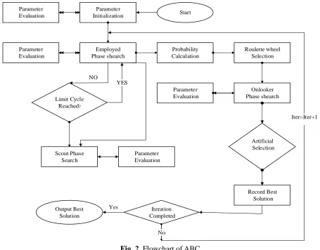
This algorithm - elevated by Karaboga [31] - is inspired by the real foraging behavior of honey bees’ colony. In this algorithm, the major objective is to investigate the most appropriate food resources in order to feed the hive. This algorithm has three vital components: (a) food resources (b) employed bees (c) unemployed bees made up of two distinct groups called scout bees and onlooker bees. More details about foraging behavior of honey bees can be observed in [31-33].

First step: Opting initial food resource position. In this algorithm, food resources play the role of answers in an optimization problem and the amount of nectar for a specific food resource is illustrative of the fitness among answers. This algorithm will be initiated by choosing initial random answers based on following equation:

 





min max min

ij j rand 0,1 j j

x = x + × x - x ₍₂₃₎

In which, x_ij denotes the initial answers, min j x

and max j

x delineate the lower and upper bounds of answers, respectively. Parameter rand is a random number between (0, 1). Parameters i 1, 2,3,. .. , SN , and

Dispatching employed bees to food resources. In the next step, each employed bee has to work in a specific food site to adapt the food resources (answers) , as below:





ij ij ij kj ij ij

ij

φ - if R MR

if otherwise

 

  

x + x x

v =

x (24)

where vj is indicative of the new positions of food resources (new answers). In case that the new food resource has a bigger amount of nectar (fitness among answers), former resources should be replaced by new resources, but if former food resources have a wider amount of nectar, they will be kept. In Equation. (24), φ_ij is a uniformly distributed random number between SF,SF in which

SF is the scale factor and also is adapted in each cycle. According to [33] this cyclic adaptation in boundaries for φ_ij will lead to escaping from getting stuck in local minima. “ Rij” is a uniformly distributed random

positive number less than one as well. “BN” is the number of employed bees and variable k is an integer generated randomly in range (1, BN), and it is different from variable i. MR is a random number [32] between (0, 1).

Modification of food site. After generating the

j

v , a fitness parameter would be calculated according to equation. (25), f is the value of the O.F and fiti shows the quality of answers.

It is worth mentioning that this process is done for the ith resource operated by the ith employed bee.

i

i i

i

i 1

if f 0 1+ f

1+ f if f < 0 fit =

 _

   

(25)

Employing the most profitable food resource. When all the employed bees finish their process of finding profitable food resource, onlooker bees assess each of the employed bees’ information and make decisions about a resource based on its probabilistic value which is proportional to its amount of nectar.

i SN

i=1 i

n

fit p =

fit



(26)

In above probability equation, fit_i is indictor of food resource proficiency related to ith employed bee and SN is the number of employed bees.

Start Parameter

Initialization Parameter

Evaluation

Employed Phase shearch Parameter

Evaluation

Probability Calculation

Roulette wheel Selection

Parameter Evaluation

Onlooker Phase shearch Limit Cycle

Reached?

Artificial Selection Parameter

Evaluation Scout Phase

Search

Record Best Solution

Iteration Completed Output Best

Solution

Yes NO

YES

Iter=Iter+1

No

Fig. 2. Flowchart of ABC.

3. Damage Detection Process

As it was mentioned in previous sections, the damage detection process is consisted of two steps in this paper. These steps are explained in detail in this section in order that the proposed method can be further clarified. Step 1: Locating damaged elements

The proposed methodology is firstly commenced with locating probable damaged elements by means of CWT applied on vertical components of static deflection of trusses (Figure 3 and Figure 8), which, as stated before, is acquired from either modal displacement or static analysis equation. (10). Note that the deflection derived from static

analysis in ABAQUS is reported only for validation of the results. Different stages of locating damaged elements applying CWT are presented as the following:

1. Static deflections of the undamaged and damaged states are computed for the structure applying equations (10) and (12), which will appear as equations (14) and (15), respectively.

3. Vertical components are separated for both up path and down path of the structure since for truss structures, which are under consideration in this paper there are nodes on both paths.

4. The CWT should be applied on the vertical components of the previous step. However, vertical components calculated for different nodes are discrete points. In order to have a smooth static deflection graph to be acquired while diminishing the model noises (not measurement noises), the number of points are intentionally increased via cubic spline interpolation technique [34], the details of which can be observed in [35] and [36]. In this way, the static deflection graph is obtained as a spline.

5. So as to cope with edge effects, the aforementioned signal extension technique is applied on the graphs. Later at this step, the difference between undamaged and damaged structures is obtained for both up and down paths applying the following equation:

II III

Input data for CWT :_{ΔU = U - U}v v v

(27)

6. Towards a desirable performance achievement for CWT, mother wavelet coif2 with 4 vanishing moments and scale 8 is recommended [27, 28].Consequently , the average value is contemplated for spotting damaged locations (equation. (28)).



CWT



_avarage=0.5





CWT



_{up path}+ CWT





_{down path}



₍₂₈₎

Step 2: Determining damage severities

During the first step, a number of elements might be erroneously assumed damaged since in the location of a local jump in wavelet coefficient diagram, it is not clear which of

the horizontal elements or diagonal ones are damaged; however, in the second step, this problem will be tackled by identifying damage severities by applying model updating method.

This step is comprised of an optimization-based model updating technique which utilizes static deflections of the structure as damage-sensitive parameter. The process of this step is explained in the following.

The optimization technique initiates the minimization process on the O.F of equation. (18). If the suspicious elements were not detected during the previous step, the number of unknown variables of the model updating process would have been equal to the number of elements which would have been a time consuming process given the large number of elements of the considered structures in this paper. Despite, with the approximate location of the damaged elements being detected applying the CWT in the first step, the number of variables diminishes to the number of suspicious elements. When the optimization algorithm is terminated, the inverse problem of finding damage severities is solved. That is, the damage values are computed for the suspicious elements. As it was stated before, all elements in the vicinity of singularities in the wavelet plot are considered suspicious. After this step, the damage severities associated with those elements which are mistakenly reported as suspicious will be reported as zero. In this way, the problem of finding damage values can be solved along with a considerable decrease in both the number of variables and the time required for the algorithm to be terminated.

modal data rather than those resulted from static analysis equation. (10) Mainly because extracting static deflections for a structure involves static actuation, which is a laborious task.

4. Illustrative Examples

Two large truss structures are modeled to evaluate the performance of the proposed technique.

To evaluate the usability of the presented method in experimental testing, different levels of noise are added to natural frequencies in both steps by using equation. (29).

 

d d





i _noisy i 1+ n.

 = . ξ ₍₂₉₎

Wherendetermines the noise level, ξ is a random real number in range (-1, 1) produced with MATLAB and id is the natural

frequency related to damaged structure for the ith mode.

Material density for the numerical examples is assumed to be 78500 N/m3, Elastic modulus is presumed2 10 11N/m2, and truss elements are contemplated prismatic. In order to attain the static deflection of the truss in static state, a

linear static analysis is performed in ABAQUS software and a modal analysis is performed in MATLAB in both of which a unit load is applied on each degree of freedom

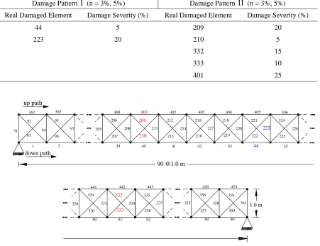
4.1. A Warren Truss with 60 Spans: Damage Detection in a 60- Span Warren Truss

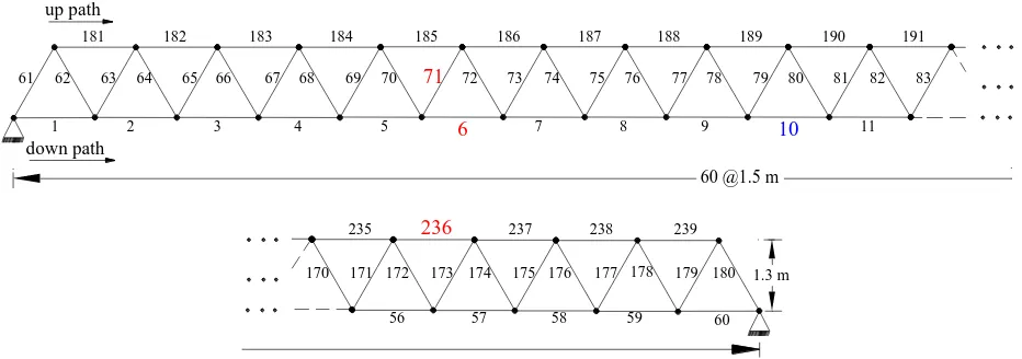
In the following example, a 60-span Warren truss with 4 simple supports containing 2 middle supports and 90 meters total length is modeled and depicted in Figure 3. As it is illustrated in Figure 3, all elements are equal in size and are of 1.5 meters length. Horizontal elements for both down path and up path have area of 200cm2 and each diagonal element is of 150cm2 cross-sectional area. The way of numbering the elements is explicated in Figure 3. It should be noted that the aggregate number of elements in this model is 239, so if model updating method was utilized individually, the number of variables would have been 239. However, by applying this two-step method, the number of variables has considerably diminished to five in scenario one and 10 in the second scenario (Table 2).

181

1 2

61 62 63 64 182

up path

down path

3 4 5 ₆ 7 8 9 ₁₀ 11

65 66 67 68 69 70 71 72 73 74 75 76 77 78 79 80 81 82 83

183 184 185 186 187 188 189 190 191

60 @1.5 m

59 60

177 178 179 180 238 239

1.3 m 237

236

176 175 174 173 172 235

171 170

58 57

56

Table 1. Model 1 damage scenarios with aggregate 239 elements

Damage Pattern  (n = 3%, 5%) Damage Pattern  (n = 3%, 5%)

Damaged Element Damage Severity (%) Damaged Element Damage Severity (%)

10 10 6 20

71 25

236 15

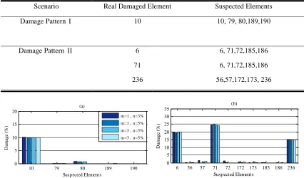
Two damage patterns are explained in Table 1 first of which possesses one impaired element and the second one has 3 impaired elements. It should be noted that the damaged element’s number for the first scenario is presented in blue color in Figure 3, and damaged elements

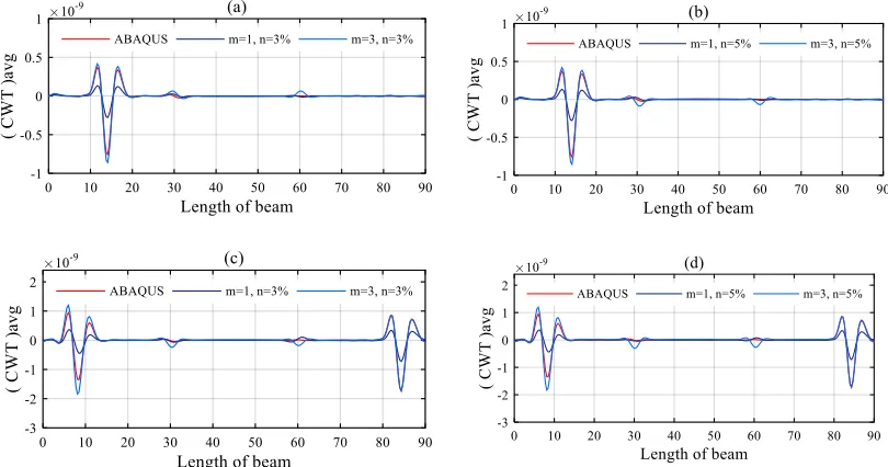
of the second scenario are shown in red. First, CWT is applied on up path and down path deflections separately and then, their average value is given in Figure 4 for damage localization. In this section the first and the first three modes are employed.

Fig. 4. Average wavelet coefficients for up and down path for model 1: (a) scenario 1 with

3% noise, (b) scenario 1 with 5% noise, (c) scenario 2 with 3% noise, (d) scenario 2 with 5% noise.

According to Figure 4, all of the diagrams reveal the location of damages in which local jumps in wavelet coefficients are, indeed, illustrative of impairments. But it should be taken into account that it is not still crystal clear that which of the horizontal or diagonal elements are damaged. In this respect, all

elements in location of local jumps are nominated as damaged and reported in Table 2.

determines which of the suspected elements are impaired. As it is vivid in Figure 5, during the second step, the model updating method successfully divulges the severity of damages in suspected elements leading to clarifying which of the suspected elements were impaired. In this process, the first and the first

three modes with two levels of additive noise are utilized. The number of particles is equal to 100 and number of iterations is 2500. Note that there is no recommendable strategy for selecting these parameters and they should be chosen by trial and error.

Table 2. Suspected elements for the 60-span Warren truss (Results of the first step)

Scenario Real Damaged Element Suspected Elements

Damage Pattern  10 10, 79, 80,189,190

Damage Pattern  6 6, 71,72,185,186

71 6, 71,72,185,186

236 56,57,172,173, 236

10 79 80 189 190

0 5 10 15 20

(a)

Suspected Elements

D

am

age

(%)

m=1 , n=3%

m=1 , n=5%

m=3 , n=3%

m=3 , n=5%

6 56 57 71 72 172 173 185 186 236 0

5 10 15 20 25 30 35

(b)

Suspected Elements

D

am

age

(%)

m=1 , n=3%

m=1 , n=5% m=3 , n=3%

m=3 , n=5%

Fig. 5. Damage severities for suspected elements in model 1: (a) scenario 1 with 3% and 5%

noise, (b) scenario 2 with 3% and 5% noise. In order to compare the efficacy, accuracy and

robustness of ABC algorithm, two other optimization algorithms, standard PSO [37] and IWO, [38] are recruited. In this respect, the first five vibration modes with 3% and 5% noise and 2500 iterations are applied and the results are given in Figure 6. According to these results, not only has ABC succeeded in

finding the correct damaged elements, but it has stated slightly more precise results in comparison with PSO and IWO as well. However, note that all the three mentioned algorithms reached acceptable damage values, which is illustrative of employing a robust O.F.

10 79 80 189 190

0 5 10 15 20

Suspected Elements

D

am

age

(%)

(a)

ABC, m=5 , n=3%

IWO, m=5 , n=3%

PSO , m=5 , n=3%

10 79 80 189 190

0 5 10 15 20

Suspected Elements

D

am

age

(%)

(b)

ABC , m=5 , n=5%

6 56 57 71 72 172 173 185 186 236 0

5 10 15 20 25 30 35

Suspected Elements

D

am

age

(%)

(c)

ABC , m=5 , n=3%

IWO , m=5 , n=3% PSO , m=5 , n=3%

6 56 57 71 72 172 173 185 186 236 0

5 10 15 20 25 30 35

Suspected Elements

D

am

age

(%)

(d)

ABC , m=5 , n=5%

IWO, m=5 , n=5% PSO , m=5 , n=5%

Fig. 6. Damage severities resulted from ABC, IWO and PSO for model 1 (a) with 3% noise –

scenario 1, (b) with 5% noise scenario 1, (c) with 3% noise – senario2, (d) with 5% noise – scenario 2.

Convergence curves affiliated with the three aforementioned optimizers, ABC, IWO and PSO are plotted for both assumed damage patterns of the first model, as depicted in Figure 7. It can be vividly obsereved from Figure 7 that even though noise is imposed in the calculations, ABC is converged to the least value almost after 400 iterations in the first scenario (Figure 7(a), (b)). In the convergence curve of the second scenario (Figure 7(c), (d)), it can be observed that

ABC algorithm reached the optimum answer almost after 1500 iterations, which is longer in comparison with the first scenario. This is due to increase in the number of variables; that is, it is five in the second scenario versus one in the first scenario. Thus, it can be interpreted that a positive correlation does exist between the number of variables and the number of iterations required for converging to optimum answers.

0 500 1000 1500 2000 2500

10-20 10-15 10-10 10-5

Number of Iteration

Cos

t

(a)

ABC , m=5 , n=3%

IWO, m=5 , n=3%

PSO , m=5 , n=3%

0 500 1000 1500 2000 2500 10-20

10-15 10-10 10-5

Number of Iteration

Cos

t

(b)

ABC , m=5 , n=5% IWO , m=5 , n=5% PSO , m=5 , n=5%

0 500 1000 1500 2000 2500

10-20 10-15 10-10 10-5

Number of Iteration

Cos

t

(c)

ABC , m=5 , n=3%

IWO, m=5 , n=3% PSO , m=5 , n=3%

0 500 1000 1500 2000 2500 10-15

10-10 10-5

Number of Iteration

Cos

t

(d)

ABC , m=5 , n=5% IWO , m=5 , n=5% PSO , m=5 , n=5%

Fig. 7. Convergence curves for model 1 for which the first five modes are considered a) with

4.2. Damage Detection in a 90-Span Brown Truss

In order to highlight the effectiveness of the proposed method, a 90-span Brown truss with four simple supports including two middle supports is modeled. Figure 8 portrays this truss with 90 meters length and

one meter height. Cross sectional area is 200cm2 for horizontal elements located in either up path or down path and 150cm2 for vertical and diagonal elements. Total number of truss elements in this model is 451.

Table.3: Model 2 damage scenarios with aggregate 451 elements

Damage Pattern  (n = 3%, 5%) Damage Pattern  (n = 3%, 5%)

Real Damaged Element Damage Severity (%) Real Damaged Element Damage Severity (%)

44 5 209 20

223 20 210 5

332 15

333 10

401 25

1 2 39 40

91 92

93

362 363 95

96

94 97 211

401

209

210

400 206

207 208 205

up path

down path

89 90

361 451 359

360 450

356

357

358 _{1.0 m}

41 42

217 403 215

216 402

212

213 214

43 44

223

405 221

222 404

218

219 220

45 406 224

225 226

82 337 443 335

336 334

80 81

442

332

333

441 329

330 331

328 355

90 @1.0 m

Fig. 8. Model 2: A Brown truss with 90 meters length with 4 simple supports including 2 middle supports

Two damage patterns are contemplated (see Table 3). Similar to the previous numerical example, damaged elements are highlighted by blue numbers for the first scenario, and red for the second scenario in Figure. In the first scenario, one vertical and one horizontal

located. Unlike the first scenario, static deflection resulted from the first five modes is applied in the second scenario and damaged regions are revealed in forms of

local jumps (Figure 9(c), (d)). The suspected elements which are the input data for the second step are listed in Table 4.

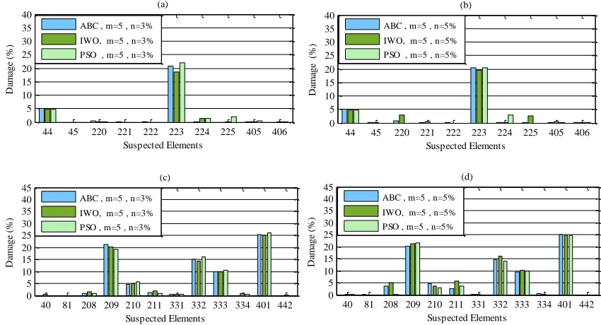
Table 4. Suspected elements for the 90-span Brown truss (Results of the first step).

Scenario Real Damaged Element Suspected Elements

Damage Pattern  44 44,45,220,221,222,223,224,225,405,406

223 44,45,220,221,222,223,224,225,405,406

Damage Pattern  209 40,208,209,210,211,401

210 40,208,209,210,211,401

332 81,331,332,333,334,442

333 81,331,332,333,334,442

401 40,208,209,210,211,401

Fig. 9. Average wavelet coefficients for up and down path for model 2: (a) scenario 1 with 3% noise,

(b) scenario 1 with 5% noise, (c) scenario 2 with 3%, (d) scenario 2 with 5% noise.

Similarly, in the second step of the approach, damage severities are computed by employing model updating by means of the

damaged elements will be distinguished from undamaged ones by reporting damage

severities for nominated elements.

44 45 220 221 222 223 224 225 405 406 0 5 10 15 20 25 30 35 (a) Suspected Elements D am age (%)

m=1 , n=3%

m=1 , n=5%

m=3 , n=3%

m=3 , n=5%

40 81 208 209 210 211 331 332 333 334 401 442 0 5 10 15 20 25 30 35 (b) Suspected Elements D am age (%)

m=1 , n=3%

m=1 , n=5% m=3 , n=3%

m=3 , n=5%

Fig. 10. Damage severities for suspected elements generated by model updating process with

ABC algorithm for model 2: (a) scenario 1 with 3% and 5% noise, (b) scenario 2 with 3% and 5% noise.

In order for comparing the performance, accuracy and robustness of ABC with other algorithms, the second step is done for both scenarios by IWO and PSO in all of which the first five modes are utilized. In this process, modal data are contaminated with 3 % and 5% noise and the number of iterations

is assumed to be 2500. Based on the results illustrated in Figure 11, ABC algorithm is better in both accuracy and robustness than standard PSO and IWO. One even could observe in Figure 11(d) that IWO has mistakenly detected elements 208 and 211 as about 5% and 6% damaged, respectively.

44 45 220 221 222 223 224 225 405 406 0 5 10 15 20 25 30 35 40 Suspected Elements D am age (%) (a)

ABC , m=5 , n=3%

IWO, m=5 , n=3% PSO , m=5 , n=3%

44 45 220 221 222 223 224 225 405 406 0 5 10 15 20 25 30 35 40 Suspected Elements D am age (%) (b)

ABC , m=5 , n=5%

IWO, m=5 , n=5% PSO , m=5 , n=5%

40 81 208 209 210 211 331 332 333 334 401 442 0 5 10 15 20 25 30 35 40 45 Suspected Elements D am age (%) (c)

ABC , m=5 , n=3%

IWO, m=5 , n=3% PSO , m=5 , n=3%

40 81 208 209 210 211 331 332 333 334 401 442 0 5 10 15 20 25 30 35 40 45 Suspected Elements D am age (%) (d)

ABC , m=5 , n=5%

IWO, m=5 , n=5% PSO , m=5 , n=5%

Fig. 11. Damage severities resulted from ABC, IWO and PSO– model 2 (a) with 3% noise –

scenario 1 (b) with 5% noise scenario 1 (c) with 3% noise – senario2, (d) with 5% noise – scenario 2.

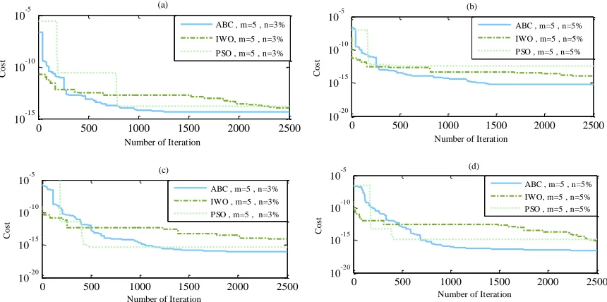
In order to consider an optimization algorithm efficient and applicable, it should

it indicates a stable, gradual converging behavior and better final cost values. For instance, as it is observable in Figure 12 that after 1250 iterations both PSO and ABC almost reached a plateau; Notwithstanding, final cost value for ABC is less than that of

PSO. In addition to that, PSO has an unstable and unpredictable behavior. Thus, according to Figure 12, it is illustrated that ABC has a superior performance in finding the best solution despite the complexity of the problem and presence of noise.

0 500 1000 1500 2000 2500

10-15 10-10 10-5

Number of Iteration

Cos

t

(a)

ABC , m=5 , n=3%

IWO, m=5 , n=3%

PSO , m=5 , n=3%

0 500 1000 1500 2000 2500

10-20 10-15 10-10 10-5

Number of Iteration

Cos

t

(c)

ABC , m=5 , n=3% IWO , m=5 , n=3% PSO , m=5 , n=3%

0 500 1000 1500 2000 2500 10-20

10-15 10-10 10-5

Number of Iteration

Cos

t

(b)

ABC , m=5 , n=5% IWO , m=5 , n=5% PSO , m=5 , n=5%

0 500 1000 1500 2000 2500

10-20 10-15 10-10 10-5

Number of Iteration

Cos

t

(d)

ABC , m=5 , n=5% IWO, m=5 , n=5% PSO , m=5 , n=5%

Fig. 12. Convergence curves for model 2 (a) with 3% noise – scenario 1 (b) with 5% noise

scenario 1 (c) with 3% noise – senario2, (d) with 5% noise – scenario 2.

5. Concluding Remarks

The present article propounds a two-step technique comprised of WT and model updating method for damage diagnosis in large trusses. More specifically, this two-step method divides the damage detection process into two separate subsequent approaches in pursuit of reducing the number of variables in the inverse problem, especially for large structures with large number of elements. In the first step, a number of locations will be nominated as damaged via continuous wavelet transform, and in the next step, the inverse problem will be solved with optimization algorithm. It is noteworthy to mention that the performance of the proposed method is heavily dependent on both the number of

congruity with the proposed method and more stable behavior.

REFERENCES

[1] Yan, Y. J., Cheng, L., Wu, Z. Y., Yam, L. H. (2007). Development in vibration-based structural damage detection technique. Mechanical Systems and Signal Processing, 21(5), 2198-2211.

[2] Fan, W., Qiao, P. (2011). Vibration-based damage identification methods: a review and comparative study. Structural Health Monitoring, 10(1), 83-111.

[3] Liew, K. M., Wang, Q. (1998). Application of wavelet theory for crack identification in structures. Journal of engineering mechanics, 124(2), 152-157.

[4] Li, B., Chen, X. (2014). Wavelet-based numerical analysis: a review and classification. Finite Elements in Analysis and Design, 81, 14-31.

[5] Altammar, H., Dhingra, A., Kaul, S. (2014). Use of Wavelets for Mixed-mode Damage Diagnostics in Warren Truss Structures. In ASME 2014 International Design Engineering Technical Conferences and Computers and Information in Engineering Conference (pp. V008T11A001-V008T11A001). American Society of Mechanical Engineers.

[6] Bagheri, A., Ghodrati Amiri, G., Khorasani, M., Bakhshi, H. (2011). Structural damage identification of plates based on modal data using 2D discrete wavelet transform. Structural Engineering and Mechanics, 40(1), 13-28.

[7] Yan, G., Duan, Z., Ou, J., De Stefano, A. (2010). Structural damage detection using

residual forces based on wavelet transform. Mechanical Systems and Signal Processing, 24(1), 224-239.

[8] Ghodrati Amiri, G., Jalalinia, M., Zare Hosseinzadeh, A., Nasrollahi, A. (2015). Multiple crack identification in Euler beams by means of B-spline wavelet. Archive of Applied Mechanics, 85(4), 503-515.

[9] Yang, C., Oyadiji, S. O. (2017). Damage detection using modal frequency curve and squared residual wavelet coefficients-based damage indicator. Mechanical Systems and Signal Processing, 83, 385-405.

[10] Abbasnia, R., Mirzaei, B., Yousefbeik, S. (2016). A two-step method composed of wavelet transform and model updating method for multiple damage diagnosis in beams. Journal of Vibroengineering, 18(3). [11] Ravanfar, S. A., Razak, H. A., Ismail, Z., Hakim, S. J. S. (2015). A Hybrid Procedure for Structural Damage Identification in Beam-Like Structures Using Wavelet Analysis. Advances in Structural Engineering, 18(11), 1901-1913. [12] Carden, E. P., Fanning, P. (2004). Vibration based condition monitoring: a review. Structural health monitoring, 3(4), 355-377.

[13] Marwala, T. (2010). Finite element model updating using computational intelligence techniques: applications to structural dynamics. Springer Science & Business Media.

[15] Kaveh, A., Maniat, M. (2014). Damage detection in skeletal structures based on charged system search optimization using incomplete modal data. International journal of civil engineering IUST, 12(2), 291-298.

[16] Tabrizian, Z., Ghodrati Amiri, G., Hossein Ali Beigy, M. (2014). Charged system search algorithm utilized for structural damage detection. Shock and Vibration, 2014.

[17] Kaveh, A., Maniat, M. (2015). Damage detection based on MCSS and PSO using modal data. Smart structures and systems, 15(5), 1253-70.

[18] Majumdar, A., Nanda, B., Maiti, D. K., Maity, D. (2014). Structural damage detection based on modal parameters using

continuous ant colony

optimization. Advances in Civil Engineering, 2014.

[19] Ding, Z. H., Huang, M., Lu, Z. R. (2016). Structural damage detection using artificial bee colony algorithm with hybrid search strategy. Swarm and Evolutionary Computation, 28, 1-13.

[20] Xu, H., Ding, Z., Lu, Z., (2015). Structural damage detection based on Chaotic Artificial Bee Colony algorithm, Structural Engineering and Mechanics 55: 1223-1239.

[21] Kaveh, A., Vaez, S. R. H., Hosseini, P., & Fallah, N. (2016). Detection of damage in truss structures using Simplified Dolphin Echolocation algorithm based on modal data. Smart Structures and Systems, 18(5), 983-1004.

[22] Ghodrati Amiri, G., Zare Hosseinzadeh, A., Jafarian Abyaneh, M. (2015). A New

Two-Stage Method for Damage Identification in Linear-Shaped Structures Via Grey System

Theory and Optimization

Algorithm. Journal of Rehabilitation in Civil Engineering, 3(2), 45-58.

[23] Zhu, J. J., Li, H., Lu, Z. R., Liu, J. K. (2015). A Two-Step Approach for Structural Damage Localization and Quantification Using Static and Dynamic Response Data. Advances in Structural Engineering, 18(9), 1415-1425.

[24] Mallat, S., Hwang, W. L. (1992). Singularity detection and processing with wavelets. IEEE transactions on information theory, 38(2), 617-643.

[25] Mallat, S. (2008). A wavelet tour of signal processing: the sparse way. Burlington, MA Academic press.

26] Misiti, M., Misiti, Y., Oppenheim, G., (1996). Wavelet toolbox. The MathWorks Inc., Natick, MA.

[27] Montanari, L., Basu, B., Spagnoli, A., Broderick, B. M. (2015). A padding method to reduce edge effects for enhanced damage identification using wavelet analysis. Mechanical Systems and Signal Processing, 52, 264-277.

[28] Montanari, L., Spagnoli, A., Basu, B., & Broderick, B. (2015). On the effect of spatial sampling in damage detection of cracked beams by continuous wavelet transform. Journal of Sound and Vibration, 345, 233-249.

[29] Messina, A. (2008). Refinements of damage detection methods based on wavelet

analysis of dynamical

[30] Zare Hosseinzadeh, A., Ghodrati Amiri, G., & Koo, K. Y. (2016). Optimization-based method for structural damage localization and quantification by means of static displacements computed by flexibility matrix. Engineering Optimization, 48(4), 543-561.

[31] Karaboga, D. (2005). An idea based on honey bee swarm for numerical optimization (Vol. 200). Technical report-tr06, Erciyes university, engineering faculty, computer engineering department. [32] Karaboga, D., & Akay, B. (2011). A

modified artificial bee colony (ABC) algorithm for constrained optimization problems. Applied Soft Computing, 11(3), 3021-3031.

[33] Akay, B., & Karaboga, D. (2012). A modified artificial bee colony algorithm

for real-parameter

optimization. Information Sciences, 192, 120-142.

[34] Solís, M., Algaba, M., & Galvín, P. (2013). Continuous wavelet analysis of mode shapes differences for damage detection. Mechanical Systems and Signal Processing, 40(2), 645-666.

[35] Rucka, M., & Wilde, K. (2006). Crack identification using wavelets on experimental static deflection profiles. Engineering structures, 28(2), 279-288.

[36] Radzieński, M., Krawczuk, M., & Palacz, M. (2011). Improvement of damage detection methods based on experimental modal parameters. Mechanical Systems and Signal Processing, 25(6), 2169-2190. [37] Kennedy, J., Eberhart, R.C., (1995). Particle

swarm optimization, Proceedings of the

IEEE international conference on neural networks, Piscataway, NJ1942-1948. [38] Mehrabian, A. R., & Lucas, C. (2006). A

novel numerical optimization algorithm

inspired from weed