https://doi.org/10.5194/gmd-12-4185-2019 © Author(s) 2019. This work is distributed under the Creative Commons Attribution 4.0 License.
Pysteps: an open-source Python library for probabilistic
precipitation nowcasting (v1.0)
Seppo Pulkkinen1,2, Daniele Nerini3,4, Andrés A. Pérez Hortal5, Carlos Velasco-Forero6, Alan Seed6, Urs Germann3, and Loris Foresti3
1Colorado State University, Fort Collins, CO, USA 2Finnish Meteorological Institute, Helsinki, Finland
3Federal Office of Meteorology and Climatology MeteoSwiss, Locarno-Monti, Switzerland 4Institute for Atmospheric and Climate Science, ETH Zurich, Zurich, Switzerland
5Department of Atmospheric and Oceanic Sciences, McGill University, Montreal, Canada 6Bureau of Meteorology, Melbourne, Australia
Correspondence:Seppo Pulkkinen ([email protected]) Received: 5 April 2019 – Discussion started: 13 May 2019
Revised: 8 August 2019 – Accepted: 25 August 2019 – Published: 7 October 2019
Abstract.Pysteps is an open-source and community-driven Python library for probabilistic precipitation nowcasting, that is, very-short-range forecasting (0–6 h). The aim of pysteps is to serve two different needs. The first is to provide a modular and well-documented framework for researchers interested in developing new methods for nowcasting and stochastic space–time simulation of precipitation. The second aim is to offer a highly configurable and easily accessible platform for practitioners ranging from weather forecasters to hydrol-ogists. In this sense, pysteps has the potential to become an important component for integrated early warning systems for severe weather.
The pysteps library supports various input/output file for-mats and implements several optical flow methods as well as advanced stochastic generators to produce ensemble now-casts. In addition, it includes tools for visualizing and post-processing the nowcasts and methods for deterministic, prob-abilistic and neighborhood forecast verification. The pys-teps library is described and its potential is demonstrated us-ing radar composite images from Finland, Switzerland, the United States and Australia. Finally, scientific experiments are carried out to help the reader to understand the pysteps framework and sensitivity to model parameters.
1 Introduction
As defined by the World Meteorological Organization (WMO), nowcasting encompasses a description of the cur-rent state of the atmosphere along with forecasts up to 6 h ahead (Wang et al., 2017). These short-term forecasts, typ-ically obtained by extrapolation of observations, statistical models or numerical weather prediction (NWP), represent an essential tool to predict severe weather, such as heavy precip-itation and intense thunderstorms.
Excessive rainfall can act as a trigger for water-related haz-ards (Alfieri et al., 2012), and this is particularly true in an in-creasingly urbanized territory or in the presence of steep to-pography. When vulnerable objects become exposed to such hazards, risk can manifest in terms of property damage and loss of lives.
1.1 From deterministic to probabilistic nowcasting Weather radars are ideally suited for providing the input data for precipitation nowcasting at high resolution, namely spa-tial scales under 2 km and time ranges between 5 min and 3 h (Berne et al., 2004). Despite recent advances in numeri-cal weather prediction (e.g., Sun et al., 2014), extrapolation-based nowcasting remains the primary approach at such space- and timescales, typically outperforming NWP fore-casts in the first 2–5 h, depending on the weather situa-tion, domain and NWP characteristics (e.g., Berenguer et al., 2012; Mandapaka et al., 2012; Simonin et al., 2017; Jacques et al., 2018). Other recent developments include machine learning methods, for which promising results have been ob-tained (e.g., Xingjian et al., 2015; Foresti et al., 2019), but these have not so far been deployed in operational nowcast-ing systems.
Precipitation exhibits variability over a wide range of space- and timescales (e.g., Lovejoy and Schertzer, 2013) which, in combination with the chaotic nature of the atmo-sphere (e.g., Lorenz, 1996), limits our ability to predict its evolution in a deterministic manner. The NWP community recognized this challenge in the early 1990s and tackled the problem by producing an ensemble of NWP forecasts by per-turbing the set of initial conditions (e.g., Toth and Kalnay, 1997). Those perturbations grow exponentially and lead to an ensemble of solutions that reflect forecast uncertainties. The information contained in the ensemble can then be used to derive probabilistic forecasts.
Just as any other forecasting technique, the skill of radar-based nowcasting was found to depend on multiple factors such as the meteorological conditions, geographical location, spatial and temporal scales (e.g., Germann and Zawadzki, 2002; Foresti and Seed, 2014; Atencia et al., 2017; Mejsnar et al., 2018). It is therefore not surprising that also the now-casting community rapidly acknowledged the importance of estimating predictive uncertainty (e.g., Seed, 2003; Germann and Zawadzki, 2004; Bowler et al., 2006). A common ap-proach is based on stochastic simulation, in which correlated noise fields are used to perturb a deterministic nowcast (e.g., Bowler et al., 2006; Berenguer et al., 2011; Liguori and Rico-Ramirez, 2014; Foresti et al., 2016). Substantial research ef-forts have been made to make the perturbation fields as real-istic as possible and consistent with the nowcast uncertainty (e.g., Seed et al., 2013; Nerini et al., 2017). For a review of the history of nowcasting starting from the 1950s, and its evolution to the probabilistic framework, we refer the reader to Pierce et al. (2012).
1.2 The pysteps open-source initiative
Similarly to other research fields, the nowcasting com-munity has invested a significant amount of time to re-implement from scratch routines and algorithms that have been around for decades, for example, optical flow and
ad-vection schemes. Part of this problem is due to the unavail-ability of software, which is often proprietary or too poorly documented to be understood, trusted and used.
Recognizing that nowcasting methods and related appli-cations can be further developed and distributed by pro-moting universal access to existing knowledge, a Python-based software package, called pysteps, is being devel-oped as a community-driven effort. Such effort fits well into the weather radar community with emergence of open data and an increasing number of open-source software projects (Heistermann et al., 2015), for instance, in radar data processing (Heistermann et al., 2013; Helmus and Collis, 2016). More recently, community-based initiatives dedicated to nowcasting have emerged, for example, Com-SWIRLS by the Regional Specialized Meteorological Centre (RSMC) for Nowcasting operated by the Hong Kong Observatory (HKO), IMPROVER by the UK MetOffice or rainymotion at the Uni-versity of Potsdam (see Table 1).
In this article, we present pysteps, an open-source and community-driven Python library for probabilistic precipita-tion nowcasting. The objective of pysteps is two-fold. First, it aims at providing a well-documented and modular frame-work for development of new nowcasting methods. In this sense, pysteps promotes the adoption of open-science prac-tices, as the lack of common standards, transparency, code availability and well-documented workflows in computa-tional disciplines can lead to non-reproducible results, hence questioning their scientific value (Hutton et al., 2016). Sec-ond, pysteps aims at providing an easily accessible software package for practitioners ranging from weather forecasters to hydrologists.
1.3 Outline of the paper
The paper is structured as follows. The theoretical framework for precipitation nowcasting and using stochastic perturba-tions to characterize the uncertainty is formulated in Sect. 2. The general architecture of the pysteps library is presented in Sect. 3. A comprehensive verification of pysteps nowcasts is given in Sect. 4. Various experiments to understand the sen-sitivity of pysteps to the model parameters and define the de-fault configuration are done in Sect. 5. The limits of pysteps are tested in Sect. 6 using a tropical cyclone and severe con-vection case in Australia. Section 7 concludes the paper and lists potential future applications of pysteps. Finally, code listings demonstrating the use of pysteps are given in Ap-pendix A.
2 Formulation of precipitation nowcasting
Table 1.Non-exhaustive list (in alphabetical order) of precipitation nowcasting packages that are in principle available to the public. Open-source libraries have their Open-source code available to the general public. Free-license libraries can be obtained upon request.
Library Language Website Availability Reference
Com-SWIRLS Python, C++ https://com-swirls.org Open source∗ Wong et al. (2016) (last access: 23 September 2019)
IMPROVER Python, Shell https://improver.readthedocs.io Open source Flowerdew (2018) (last access: 23 September 2019)
INCA C, Fortran, Shell https://www.zamg.ac.at Free license Haiden et al. (2011) (last access: 23 September 2019)
pysteps Python https://pysteps.github.io Open source This study (last access: 23 September 2019)
rainymotion Python https://github.com/hydrogo/rainymotion Open source Ayzel et al. (2019) (last access: 23 September 2019)
STEPS C, C++ https://www.bom.gov.au Free license Bowler et al. (2006), (last access: 23 September 2019) Seed et al. (2013)
∗Only for national meteorological and hydrological services within WMO.
2.1 Lagrangian persistence and optical flow
In its simplest form, extrapolation-based precipitation now-casting assumes that over the time frame of a few hours the evolution of precipitation can be captured by moving the radar echoes along a stationary motion field without changes in intensity. In the literature, this is known as Lagrangian per-sistence (Zawadzki et al., 1994).
Denoting a precipitation parcel byRand its displacement vector byα(τ ), the conservation equation for an incompress-ible flow is written as
R(x0;t+τ )=R(x0−α(τ );t ), (1)
or equivalently in differential form as dR
dt = ∂R
∂t +u ∂R
∂x +v ∂R ∂y, u=
dx
dt, v=
dy
dt, (2)
where dR/dt=0, anduandvare thexandycomponents of the motion field. In the so-called optical flow methods,uand
vare estimated for a given location by solving Eq. (2) numer-ically based on a sequence of precipitation intensity fields. Typically, a constraint on the spatial continuity of nearby u
andv is imposed to guarantee a unique solution. Once the motion field is known, the radar echoes are extrapolated by means of an advection scheme.
Three methods are currently implemented in pysteps for motion field estimation: a local Lucas–Kanade method (Lu-cas and Kanade, 1981; Bouguet, 2001), a global variational echo-tracking approach (Laroche and Zawadzki, 1994; Ger-mann and Zawadzki, 2002) and a spectral approach (DARTS, Ruzanski et al., 2011). The currently implemented advection method is the backward-in-time semi-Lagrangian scheme de-scribed in Germann and Zawadzki (2002), which is robust against numerical diffusion.
2.2 Sources of uncertainty
The predictability of the atmosphere is intrinsically limited by the fact that its state cannot be observed with absolute pre-cision nor expressed without approximations in its governing laws (Lorenz, 1996). In the case of radar-based precipitation nowcasting, predictive uncertainty originates from errors in the estimation of the current state of the rainfall and motion fields (initial state errors), and limitations of Lagrangian per-sistence as a model to predict the evolution of the rainfall and motion fields (model errors).
The main contribution to model errors in the Lagrangian approach stems from the evolution of precipitation in terms of initiation, growth, decay and termination processes that violate the steady-state assumption. Other sources of model uncertainty include the assumption of stationarity of the mo-tion field, inaccuracies due to the practical implementamo-tion of the method, as the discretization in time, space and re-flectivity, and numerical diffusion of the advection scheme (Germann et al., 2006b).
Currently, pysteps focuses on the representation of the model errors, whereas incorporation of the initial state errors in the nowcasting is left for future work.
2.3 Data transformation
Currently, pysteps assumes a log-normal distribution of rain rates by applying the logarithmic transformation
R→
10log10R, ifR≥0.1 mm h−1
−15, otherwise , (3)
that corresponds to logarithmic radar rain rates (units of dBR). The value of−15 dBR is equivalent to assigning a rain rate of approximately 0.03 mm h−1to the zeros. Hereafter,R
refers to the transformed rain rates, unless otherwise stated. Using the logarithmic transformation is motivated by the fact that rain rates are approximately log-normally dis-tributed (Crane, 1990). This has two main advantages. First, it simplifies the estimation of distribution parameters, partic-ularly with limited sample size and in the presence of mea-surement noise (Harris et al., 1997). Second, the decomposi-tion of log-transformed rainfall fields defines a multiplicative cascade, where multiplication is replaced with summation in the transformed space (Seed, 2003).
2.4 A cascade of spatial scales
It has been shown that the lifetime of precipitation relates to its spatial scale (e.g., Venugopal et al., 1999; Seed, 2003; Germann et al., 2006b), often denominated as dynamic scal-ing. Recognizing this fundamental property, Seed (2003) in-troduced the Spectral Prognosis (S-PROG) model, which laid the foundation for the development of Short-Term Ensemble Prediction System (STEPS) (Bowler et al., 2006; Seed et al., 2013). The key idea is to decompose the precipitation field into a multiplicative cascade, where the cascade levels repre-sent different spatial scales, and treat them separately in the nowcasting model.
In STEPS, the scale decomposition is done by applying a fast Fourier transform (FFT) to the input precipitation field. This is motivated by the fact that for a grid of size L×L
pixels, the radial Fourier wavenumbers |k| =qk2
x+ky2 are related to spatial scales via
radial wavenumber
(pixels)
z}|{ |k| →
wavelength
(pixels)
z}|{
L
|k| →
wavelength(km)
z }| {
L1x
|k| →
scale(km)
z }| {
L1x
2|k| , (4) where1xdenotes the grid resolution (km). Thus, the spatial scale is half the wavelength. Alternative approaches to per-form a scale decomposition include the discrete-cosine trans-form (Germann and Zawadzki, 2002; Surcel et al., 2014) or wavelets (Turner et al., 2004; Scovell, 2018).
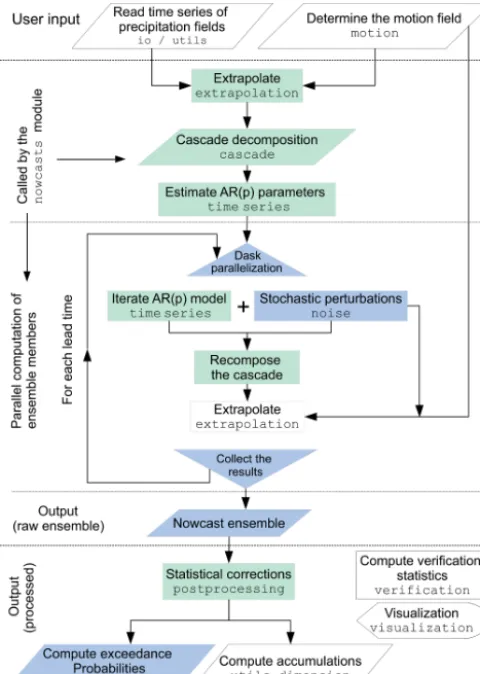
In the current implementation of pysteps, we adopt the ap-proach of Pulkkinen et al. (2018), where Gaussian weight functions are used for separating the Fourier spectrum into a set of radial bands. An example of the weight functions for the domain covered by the Finnish Meteorological Institute (FMI) radars is shown in Fig. 1. After the FFT and Gaus-sian filtering, each frequency band is transformed back to the
Figure 1.Normalized weight functions with corresponding Fourier wavenumbers and spatial scales for the FMI domain. The domain is a 760×1226 grid at 1 km resolution.
spatial domain, which results in a cascade withnlevels each representing a different scale (see an example in Fig. 2). 2.5 Temporal evolution
In nowcasting, the typical approach to model the temporal evolution of precipitation fields employs an auto-regressive (AR) process that combines the deterministic component from Lagrangian persistence with a stochastic innovation term, also referred to as a noise or perturbation term. For in-stance, S-PROG and STEPS use a second-order AR(2) pro-cess with two parameters. Separate AR(2) propro-cesses are ap-plied to each cascade level to account for the dynamic scal-ing of precipitation. The combination of the auto-regressive model in time and the cascade model in space allows one to control the temporal evolution and correlation structure of precipitation.
Currently, a more general AR(p) model has been imple-mented in pysteps. For each cascade level j, the recursion formula is given by
Rj(x, y, t )= p X
k=1
φj,kRj(x, y, t−k1t )+φj,0εj(x, y, t ). (5)
The first term corresponds to the deterministic predictable component at cascade levelj (i.e., Lagrangian persistence). The second term is a stochastic term that represents the un-predictable component at the same cascade levelj, that is, mainly initiation, growth and decay of precipitation. The symbol1t denotes the time difference between consecutive precipitation fieldsRj that are normalized to zero mean and unit variance.
Figure 2. The radar observations and seven first levels of the cascade decomposition of an FMI rain rate composite at 16:00 UTC on 28 September 2016. Values below−10 dBR were set to−15 dBR before applying the decomposition in order to reduce the discontinuity at the boundaries of precipitation areas. The observed field and the cascade levels have been normalized to zero mean and unit variance. See Listing A1 in Appendix A for obtaining the decomposition.
1,2, . . ., p using the Yule–Walker equations (Hamilton, 1994). Forp=2, the correlation coefficients can be adjusted to ensure that the resulting AR(p) process is stationary and non-periodic (Box et al., 2013). Finally, the parametersφj,0 are chosen as
φj,0= v u u t1−
p X
k=1
ρj,kφj,k. (6)
Given that the variance of the noise fields εj is one, this choice guarantees that the AR(p) process is normalized to unit variance (Hamilton, 1994).
The theoretical auto-correlation function (ACF) of the AR(2) process can be computed recursively from the model parameters and auto-correlation coefficients (Chat-field, 2003) according to
ρj(t )=φj,1ρj(t−1t )+φj,2ρj(t−21t ). (7) The empirical ACF can be derived by computing the correla-tion coefficients between the extrapolacorrela-tion nowcasts and the observations.
For an exponentially decaying ACF, the precipitation life-time is defined as the life-time when the ACF, theoretical or em-pirical, falls below the value 1/e≈0.37, whereeis the Euler number. Alternatively, one can estimate the lifetime by
inte-grating the ACF according to
T =
∞ Z
0
ρ(τ )dτ. (8)
It is not common to employ an AR(p) process withp >
2 for several reasons. First, it is not trivial to guarantee the stationarity and non-periodicity of the process. Second, when estimated in Lagrangian frame, the higher-order auto-correlation coefficients are affected by the uncertainty of the motion field. This occurs especially at small spatial scales as it is difficult to properly track convective cells over sev-eral time steps. Third, a low-order AR process is gensev-erally sufficient to model the loss of predictability in the nowcast-ing range; departures are usually observed only after≈2 h (Atencia and Zawadzki, 2014).
2.6 Stochastic perturbations of precipitation intensities The perturbation fieldεin Eq. (5) is typically generated as a correlated Gaussian random field using FFT filtering (e.g., Pegram and Clothier, 2001; Bowler et al., 2006). The process consists of three steps:
2. apply the FFT and a Fourier filter to the above to gener-ate a random field having the desired correlation struc-ture and
3. apply the inverse FFT to transform the noise field back to the spatial domain.
This technique is also known as power–law filtering of white noise or fractional integration (Schertzer and Lovejoy, 1987). At present, three methods for filtering white noise fields have been implemented in pysteps. In the absence of a model that predicts the evolution of the spatial correlation structure, one assumes that the correlation structure remains constant through the nowcast. An example is provided in Fig. 3.
In the parametric method introduced by Pegram and Cloth-ier (2001), the filtered noise fieldεis obtained from the white noise fieldεwas
ε(x, y)=F−1{f (|k|)F{εw}(kx, ky)}, (9) where F denotes the Fourier transform and the function
f defines the slope of the radially averaged power spec-trum (RAPS).
Our implementation follows the approach by Seed (2003), which uses a piecewise linear function with two spectral slopes (β1,β2) and one breaking point. The main limitation of such model relates to the assumption of an isotropic power– law scaling relationship, meaning that anisotropic structures such as rainfall bands cannot be represented.
In the non-parametric method (Seed et al., 2013), the Fourier filter is obtained directly from the power spectrum of the observed precipitation fieldRsuch that
ε(x, y)=F−1{|F{R}(kx, ky)|F{εw}(kx, ky)}. (10) Differently to the parametric method, the non-parametric approach allows generating perturbation fields with anisotropic structures. On the other hand, the approach requires a larger sample size and is sensitive to the quality of the input data, e.g., the presence of residual clutter in the radar image. In addition, both techniques assume spatial stationarity of the covariance structure of the field.
The third method is an extension of the non-parametric approach, where the noise field is generated locally to ac-count for spatial inhomogeneities in the covariance structure of the rainfall field. The technique is based on the short-space Fourier transform (SSFT) and it is described in Nerini et al. (2017). Essentially, the non-parametric approach in Eq. (10) is localized in(x, y)by
ε(x, y)=F−1{|F{Rwh(n1, n2)}(kx, ky)|F{εw}(kx, ky)}, (11)
where wh(n1, n2)=wh(n1)wh(n2) is the outer product of two Hanning windows of sizesn1andn2centered in(x, y). 2.7 Stochastic perturbations of the motion field
A second source of uncertainty in Lagrangian persistence nowcasting stems from temporal evolution of the motion
field (Germann et al., 2006b). This can be accounted for by adding stochastic perturbations. In the current implemen-tation of pysteps, this is done by applying the method of Bowler et al. (2006).
For simplicity, the perturbation field is assumed to be spa-tially constant for each ensemble member, but the magnitude of the perturbations increases with respect to lead time. For a given initial advection fieldw0and lead timet, the perturbed velocities are given by
wp(x, y)=w0(x, y)+αpar(t )εpar(x, y)wˆpar +αperp(t )εperp(x, y)wˆperp,
(12)
wherewˆpar andwˆperp denote the components parallel and perpendicular to the initial advection fieldw0, respectively. The random variables (εparandεperp) are sampled from the Laplace distribution with zero mean and unit variance. Scal-ing of the perturbations is done accordScal-ing to
αpar(t )=apartbpar+cpar (13)
αperp(t )=aperptbperp+cperp, (14)
where the parameters are climatologically fitted by using a large sample of advection fields. Example values of these pa-rameters can be found in Table 5.
2.8 Post-processing of nowcasts
To ensure that the forecast fields have the same statistical properties with the observed ones, post-processing is typi-cally done at the very end of the chain. This is necessary be-cause intermediate steps may introduce discrepancies. One major source of such discrepancies is related to the difficulty to model the intermittency of precipitation. Typically, the ba-sic statistical properties such as wet-area ratio, mean, vari-ance and the marginal distribution of precipitation intensities are assumed to remain invariant through the nowcast.
In the present implementation of pysteps, the post-processing involves two different types of methods: (1) masking and (2) matching the statistics of the forecast fields with the most recently observed ones. Methods of type (1) are used to avoid generation of stochastic cells into ar-eas that are too distant from existing precipitation. Methods of type (2) can be applied unconditionally or only to pixels within the mask.
Figure 3.Comparison of three+30 min stochastic nowcasts produced with the FFT noise generators available in pysteps as described in Sect. 2.6.(a)The radar-based rainfall analysis from the Australian radar network valid at 06:05 UTC on 1 January 2019 on a 512×512 pixel grid (event no. 2 in Table 10).(b)–(d)One member of a+30 min nowcast produced using(b)the parametric noise generator,(c)the non-parametric generator or(d)the short-space Fourier transform (SSFT) generator with a 128×128 pixel sliding window. All realizations share the same random seed.
Two methods have been implemented for matching the statistics of forecast fields with the observed ones. In the first method, which is used together with the S-PROG mask, the conditional mean of the masked forecast field is adjusted to match the conditional mean of the observed field (excluding intensities below the threshold). Alternatively, the cumula-tive distribution function (CDF) of the forecast field can be mapped to the observed one (Foresti et al., 2016). This is de-fined as
R0(x, y)=Fobs−1(F (R(x, y))), (15)
whereFobsandF denote the CDFs of the observed and the input forecast fieldR, respectively.
3 The pysteps library
3.1 Key features and development model
The implementation language of pysteps is Python (http: //python.org, last access: 23 September 2019). As a high-level language with an extensive built-in standard library and a large number of external libraries available, it is ide-ally suited for open-source software development. Python distributions, such as Anaconda, providing the necessary software to run pysteps are available for all major plat-forms. Python also provides interfaces for compiled lan-guages such as C/C++ and Fortran, allowing to improve performance in time-critical modules. In addition, Python-based tools, like the IPython shell (Pérez and Granger, 2007) or the Jupyter notebooks (https://jupyter.org, last access: 23 September 2019), allow an interactive use of pysteps for re-search and demonstration purposes.
The pysteps library is extensively documented. The doc-umentation describes in detail the different modules and the application programming interfaces (APIs). The modules are documented by using the docstring concept of Python. This is implemented using Read the docs (https://readthedocs.org/,
last access: 23 September 2019) and Sphinx (http://www. sphinx-doc.org/en/master, last access: 23 September 2019) to automatically compile and update an online version of the documentation, available at https://pysteps.readthedocs. io (last access: 23 September 2019). In addition, tutorials for performing various tasks with pysteps are included as exam-ple scripts.
Pysteps development is done by using git, a distributed version control system. The source code of pysteps is hosted in GitHub (https://pysteps.github.io, last access: 23 Septem-ber 2019). In addition to code hosting, the features of GitHub include development in multiple branches, issue tracking and wiki pages. Developers outside the core team may fork the main repository and integrate the proposed changes via pull requests, which allow community-driven development. Con-tinuous integration and testing is done by using the Travis CI framework (https://travis-ci.com/pySTEPS/pysteps, last ac-cess: 23 September 2019).
Pysteps is published under the three-clause BSD license. It allows copying, redistribution and modification of the soft-ware as long as the modification are tracked and the source code is made available under the same license. The permis-sive license model makes the software easily accessible to potential users, even allowing use for commercial purposes. 3.2 External dependencies
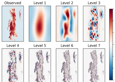
Table 2.External libraries used by pysteps.
Library Website Reference Description
h5py http://www.h5py.org
Input/output (last access: 23 September 2019)
NetCDF4 http://unidata.github.io/netcdf4-python (last access: 23 September 2019) PIL https://github.com/python-pillow/Pillow
(last access: 23 September 2019)
OpenCV http://opencv.org Bradski (2000) Image processing
(last access: 23 September 2019)
NumPy http://www.numpy.org Van Der Walt et al. (2011)
Mathematical routines (last access: 23 September 2019)
SciPy http://www.scipy.org Jones et al. (2001)
(last access: 23 September 2019)
FFTW/pyFFTW http://www.fftw.org Frigo and Johnson (2005) Fast Fourier transform (last access: 23 September 2019)
https://github.com/pyFFTW (last access: 23 September 2019)
dask http://dask.org Dask Development Team (2016) Parallelization (last access: 23 September 2019)
cartopy https://github.com/SciTools/cartopy Met Office (2010–2015)
Visualization (last access: 23 September 2019)
Matplotlib http://matplotlib.org Hunter (2007) (last access: 23 September 2019)
mpl_toolkits.basemap http://matplotlib.org/basemap (last access: 23 September 2019)
Support for NetCDF (the default file format), HDF5 and various image file formats is implemented via the NetCDF4, h5py and PIL libraries. A complete list of supported in-put/output file formats is given in the official pysteps doc-umentation. Plotting precipitation data with basemaps has been implemented via mpl_toolkits.basemap and cartopy packages. The Lucas–Kanade optical flow algorithm used in pysteps is implemented in the OpenCV library and accessed via a Python interface. Parallelized computation of nowcast ensembles is done by using Dask, which provides a platform-independent back end for low-level methods.
3.3 Key design principles
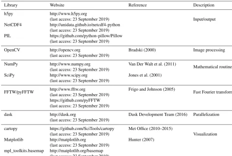
The aim of pysteps is to be a modular software library where all the main components are interchangeable. This makes the pysteps an ideal research platform for developing and testing new methods as well as a valuable tool for operational mete-orology, easily allowing the comparison of different nowcast algorithms or running multi-model ensemble nowcasts. Pys-teps is currently divided into 11 modules that perform dif-ferent tasks. The modules and their descriptions are listed in Table 3.
The modularity is implemented via interface-based design. To this end, each module implements one subtask and an
in-terface method for retrieving the desired method for this task. All mutually interchangeable methods implement the same interface. Another key principle is that whenever possible, the data are stored inn-dimensional arrays, which allow an efficient and compact representation.
The above design principles are demonstrated in the fol-lowing example. A precipitation nowcast by using STEPS can be generated by
>>> nowcast_method = nowcasts.get_method("steps") >>> nowcast = nowcast_method(R, V, num_timesteps)
where the required inputs are
R: array of shape (t, m, n) containing a time series oft
observed precipitation intensity fields with shape (m, n),
3.4 Data structures
In addition to being modular, pysteps implements object-oriented features. However, instead of using customized classes, we use dictionaries and functions that operate on the dictionaries similarly to class member functions. This design decision is motivated by the principle of using the core Python data types rather than implementing customized classes. The flat design of pysteps should facilitate user inter-action and embedding of individual modules and functions in other software. In this way, pysteps is similar to wradlib (Heistermann et al., 2013).
To demonstrate the above design, the following example shows how to construct a Gaussian bandpass filter for eight cascade levels using thefilter_gaussianfunction im-plemented in the cascade.bandpass_filters mod-ule:
>>> filter = filter_gaussian(R.shape, 8)
The output is a dictionary with three elements: (1) one-dimensional weights corresponding to the radial wavenum-bers, (2) a two-dimensional weight field for the FFT of the input image and (3) a list of central frequencies for each weight function (see Fig. 1). The resulting filter object can then be passed todecomposition_fftas follows:
>>> decomp = decomposition_fft(R, filter)
The decomposition is applied to a two-dimensional precip-itation fieldR, and the output is again a dictionary with three-elements: (1) a three-dimensional array containing the eight cascade levels having the same dimension as R, (2) mean precipitation values of each cascade level and (3) standard deviations for each level. More detailed examples of pysteps usage are provided in Appendix A.
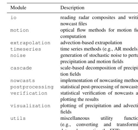
3.5 Workflow
Figure 4 illustrates the workflow for generating precipitation nowcasts using pysteps. The first step is reading the input data using the iomodule. Methods for reading radar com-posites from Australian Bureau of Meteorology (BoM), FMI, KNMI and MeteoSwiss have been implemented. In addi-tion, the importers module supports reading the European-wide OPERA radar composites in the ODIM HDF5 format. Conversion from reflectivity (dBZ) to precipitation intensity (mm h−1) and other preprocessing can be done by using the utilsmodule. Due to the modular design of pysteps, read-ing custom data formats and conversions (e.g., by usread-ing dif-ferentZ−R relationships and polarimetric parameters) can also be implemented.
Reading the input data is followed by determination of the motion field using the methods implemented in the motion module. The precipitation intensity and mo-tion fields are supplied as inputs to a user-chosen now-casting method implemented in the nowcasts module. For the Lagrangian persistence method implemented in
Table 3.Overview of pysteps modules.
Module Description
io reading radar composites and writing
nowcast files
motion optical flow methods for motion field computation
extrapolation advection-based extrapolation
timeseries time series methods (e.g., AR models)
noise generation of stochastic noise to perturb precipitation and motion fields
cascade scale-based decomposition of precipita-tion fields
nowcasts implementation of nowcasting methods
postprocessing statistical post-processing of nowcasts
verification statistical verification of nowcasts and plotting the results
visualization plotting of precipitation and advection fields
utils miscellaneous utility functions
(e.g., converting and transforming
data and computing the FFT)
nowcasts.extrapolation, the remaining step of gen-erating the nowcast is extrapolation.
When the cascade decomposition and the autoregressive model are used for scale filtering (the S-PROG model), the additional steps include those marked with green color in Fig. 4. When generating ensembles (the STEPS model), stochastic perturbations are added to the AR(p) models and to the advection field using the methods implemented in thenoisemodule. These steps are marked with blue color in Fig. 4.
The ensemble generation is parallelized by using the dask library. For each time step, this is done by splitting the com-putation to the available processor cores so that each core is responsible for computation of one ensemble member.
Figure 4. Workflow for computing precipitation nowcasts using pysteps. For each chart element, the top row describes the task and the bottom row is the name of the module used for this purpose. White colors represent the operations that are done with all now-casting methods. Green colors represent the additional operations included when the cascade decomposition and the autoregressive AR(p) model are applied (i.e., the S-PROG model). Finally, blue colors represent the operations that are done when stochastic per-turbations are added and the ensemble computation is parallelized (i.e., the full STEPS model).
4 Evaluation of nowcast quality
Verification is an essential step of forecasting, not only to monitor forecast performance over time but also to provide feedback on how to improve the model itself (diagnostic ver-ification). For an ensemble forecast, it is necessary to check whether it is unbiased and has the correct dispersion, and that the forecast probabilities are reliable and sharp (e.g., Jolliffe and Stephenson, 2003). In this section, we evaluate these attributes of pysteps ensemble nowcasts using radar composites from Switzerland and Finland, while data from the United States and Australia will also be used in Sects. 5 and 6.
Table 4.Overview of the radar quantitative precipitation estimation (QPE) composites that have been used to evaluate pysteps. The grid size is given as the number of pixels in thexandydimensions.
Dataset Country Resolution Grid size
FMI Finland 1 km, 5 min 760×1226 MeteoSwiss Switzerland 1 km, 5 min 710×640 WDSS∗ United States 4 km, 5 min 1361×1056 BoM Australia 0.5 km, 5 min 512×512
∗Upscaled from original data at 1 km resolution (5445×4226).
4.1 Description of the data
As of 2019, the radar network operated by the FMI con-sists of 10 polarimetric C-band Doppler radars. After clut-ter filclut-tering, the measured radar reflectivities are inclut-terpolated into a grid with spatial and temporal resolutions of 1 km and 5 min, respectively. The correction for the vertical pro-file of reflectivity (VPR) is applied in order to reduce range-dependent biases (Koistinen and Pohjola, 2014). Finally, re-flectivities are converted to rainfall intensities using theZ−R
relation,Z=223R1.53, adapted to the Finnish climate con-ditions (Leinonen et al., 2012). A total of 10 precipitation events from Finland containing both stratiform and convec-tive precipitation were chosen for this study (Table 7).
The latest fourth-generation MeteoSwiss network consists of five polarimetric C-band Doppler radars (Germann et al., 2015). The quantitative precipitation estimation (QPE) prod-uct used in this study includes automatic hardware calibra-tion, clutter filtering, correction for beam shielding, correc-tion for VPR effects,Z−Rrelation (Z=316R1.5) and bias adjustment (Germann et al., 2006a). The radar composite is calculated on a 1 km grid every 5 min. Overall, 10 events con-sisting of predominantly convective precipitation were cho-sen from the Swiss data (Table 8).
The US dataset comprises the radar mosaics provided by Warning Decision Support System-Integrated Information (WDSS-II Lakshmanan et al., 2006, 2007), covering the con-tinental United States at a spatial resolution of approximately 1 km. For the WDSS data, the resolution of the precipita-tion fields is upscaled from 1 to 4 km by averaging 4×4 grid points to reduce the computational requirements. The chosen precipitation events are described in Table 9.
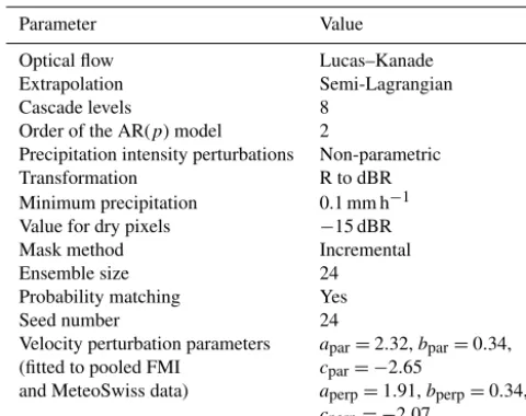
Table 5.The default configuration used in the experiments.
Parameter Value
Optical flow Lucas–Kanade
Extrapolation Semi-Lagrangian
Cascade levels 8
Order of the AR(p) model 2
Precipitation intensity perturbations Non-parametric
Transformation R to dBR
Minimum precipitation 0.1 mm h−1
Value for dry pixels −15 dBR
Mask method Incremental
Ensemble size 24
Probability matching Yes
Seed number 24
Velocity perturbation parameters apar=2.32,bpar=0.34,
(fitted to pooled FMI cpar= −2.65
and MeteoSwiss data) aperp=1.91,bperp=0.34,
cperp= −2.07
locations. The QPE grids are calculated with a spatial resolu-tion of 0.5 km every 5 min. The BoM radar dataset comprises two precipitation events: a tropical cyclone in northern Aus-tralia and a severe convective event in Sydney (Table 10).
Table 4 summarizes the different data sources and resolu-tions.
4.2 Verification metrics
Pysteps includes a number of verification metrics to help users to analyze the general characteristics of the nowcasts in terms of consistency and quality (or goodness). Probabilis-tic forecasts have been verified using the relative operating characteristic (ROC) curve, reliability diagrams and rank his-tograms, as implemented in theverificationmodule of pysteps.
The ROC curve (Jolliffe and Stephenson, 2003) measures the ability of a probabilistic forecast to discriminate between precipitation and no precipitation exceeding a given intensity threshold. For a set of probability thresholds, the ROC curve is constructed by plotting the probability of detection (POD) against the false alarm rate (POFD), not to be confused with the false alarm ratio (FAR). For a perfect forecast, the curve passes through the upper left corner (i.e., 100 % hit rate and 0 % false alarm rate). The area under the ROC curve can be used as a measure of potential skill. For more details on the contingency tables and the formulas of the categorical scores, the reader is referred to Jolliffe and Stephenson (2003).
The reliability diagram (Bröcker and Smith, 2007) mea-sures the bias (reliability) and resolution of a probabilistic forecast. For a given intensity threshold, the diagram shows the forecast probability against the observed frequencies, where the probability range[0,1]is divided intonbins. For a perfectly reliable forecast, the curve lies on the diagonal. The reliability diagram is often accompanied by a histogram
showing the sample size in each bin (sharpness diagram). A sharp forecast has few samples in the middle of the histogram and many on the sides (probability of either 1 or 0).
The rank histogram (Hamill, 2001) measures how well the ensemble spread corresponds to the observed uncertainty. For each nowcast grid pixel, the ensemble members are ranked in increasing order. A pooled histogram is computed by assigning each verifying observation a bin which it falls into among the ensemble members. The first and last bins are assigned for observations below or above all members, respectively. For a forecast ensemble whose distribution is consistent with the observations, the histogram is flat and no observations fall into the first or last bin. To handle ties (e.g., when both the observed precipitation and several en-semble members are equal to 0), we implemented the method of Hamill and Colucci (1997). The method randomly chooses a bin between(M+1)and(M+Mtied)+1, whereMis the number of members smaller than the observation andMtied is the number of ties (ensemble members equal to the obser-vation).
An additional metric that can be derived from rank his-tograms is the outlier percentage (OP). The OP measures the proportion of observations falling outside the ensemble, de-fined by
OP=h1+hn+1 Pn+1
i=1hi
, (16)
wherehi denotes theith bin of the rank histogram.
Pysteps also includes standard neighborhood verification methods, such as the fractions skill score (FSS). FSS pro-vides an intuitive assessment of the dependency of skill on spatial scale from high-resolution precipitation forecasts (Mittermaier and Roberts, 2010). The FSS is computed by comparing the forecast and observed fractional coverage of precipitation exceeding certain thresholds in spatial windows (neighborhoods) of increasing size. Using FSS it is possible to determine how the forecast skill varies with neighborhood size and then determine the smallest scale that provides a suf-ficiently skillful forecast.
4.3 Verification results
The quality of ensemble nowcasts produced by pysteps was verified by using the MeteoSwiss data and the default config-uration listed in Table 5. Using the reliability diagram, ROC curve and rank histogram as verification metrics, the results of the experiments are shown in Figs. 5–7. The results ob-tained by using the FMI data were very similar and thus not shown here.
in-Figure 5.Reliability diagrams(a)and ROC curves(b)computed from STEPS nowcasts during the MeteoSwiss events listed in Table 8 with different lead times and threshold 0.1 mm h−1. The default settings listed in Table 5 were used for computing the nowcasts. The optimal probability thresholds that maximize POD-POFD are marked in the ROC curves with black crosses.
Figure 6.Same as Fig. 5 but for an intensity threshold of 5 mm h−1.
dicates that the pysteps nowcasts are slightly overconfident (Tippett et al., 2014).
When a higher 5 mm h−1 intensity threshold is used, Fig. 6a shows a significant deviation of the reliability dia-gram from the diagonal only after 45 min, which is accom-panied by loss of sharpness. However, the ROC area remains above 0.8, indicating potentially useful skill. This suggests that more reliable nowcasts could be obtained by implement-ing additional calibration procedures in a future version of pysteps. Another observation that suggests lack of calibration is that the optimal nowcasts for precipitation/no precipitation are obtained by choosing a very low probability threshold (for a well-calibrated nowcast, this would be 0.5).
The rank histograms (Fig. 7) also show some ensemble underdispersion with larger values on the first and last bins. In general, we found that there are more misses than false alarms (i.e., cases when all members are lower than the ob-servations). This occurs, for instance, in cases of convective initiation. Despite the ability of pysteps to generate some new light random rain, it is not designed to represent the uncer-tainty related to an explosive initiation of a thunderstorm.
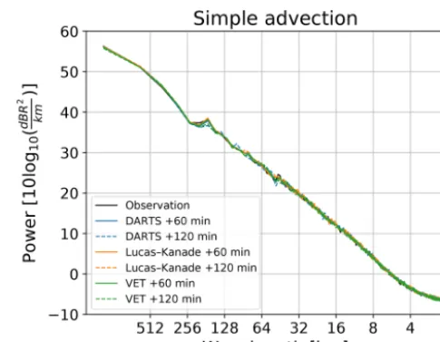
4.4 Numerical diffusion analysis
Conventional semi-Lagrangian schemes are implemented in a recursive way so that the precipitation intensities are interpolated at each time step, which usually leads to substantial numerical diffusion (i.e., loss of power at high spatial frequencies). In the pysteps method (the extrapolation.semilagrangian module), this is done by iteratively tracing the locations of precipitation parcels and interpolating the intensities only as the final step of the advection (Germann and Zawadzki, 2002).
Figure 7.Rank histograms computed from STEPS nowcasts during the MeteoSwiss events listed in Table 8 with different lead times. The default settings listed in Table 5 were used for computing the nowcasts.
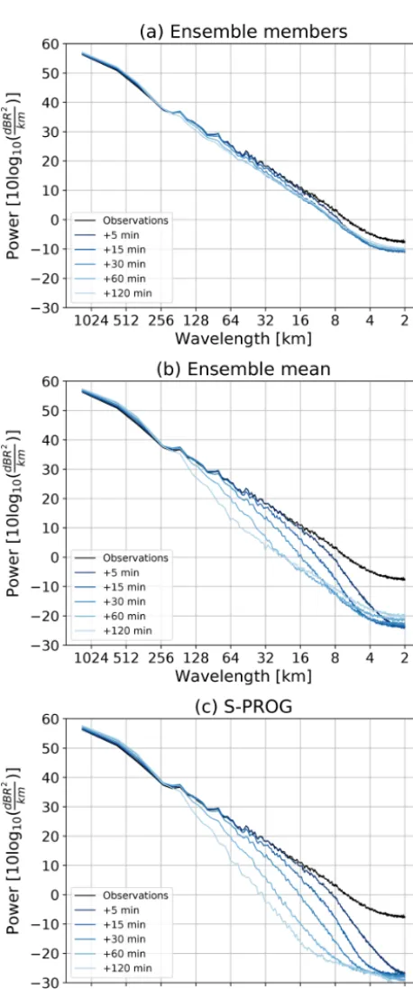
4.5 Spatial structure analysis
The aim of probabilistic nowcasting is to generate a reliable ensemble of equiprobable realizations of precipitation fields characterized by power spectra similar to those in Fig. 8. Fig-ure 9a shows the average spectra of a stochastic 48-member nowcast for FMI precipitation event no. 3. Despite a small loss of power for scales (<100 km), all spectra are close to the observations. In other words, the spatial structure of en-semble members remains realistic at all forecast lead times.
Figure 9b shows the results of the same analysis but for the ensemble mean forecast (the average of ensemble members). The process of ensemble averaging should produce precipi-tation fields that become smoother with lead time, which is the aftermath of the loss of predictability at small scales (Sur-cel et al., 2014). As expected, Fig. 9b shows a gradual loss of power at small scales. The departure of the forecast spec-tra from the observed ones occurs at increasing wavelengths, i.e.,≈16 km at 5 min and≈128 km at 60 min. However, af-ter 30 min, there is a certain increase of power at wavelengths smaller than 16–32 km. This behavior is attributed to the lim-ited ensemble size, which is not large enough to filter out pre-cipitation features at small scales. Thus, one may argue that if the ensemble is too small to model the loss of predictabil-ity at such scales, it may also be too small to reliably model the forecast uncertainty.
An alternative way to deterministically represent the fore-cast uncertainty is to filter out the unpredictable features us-ing the S-PROG model (Fig. 9c). Also, in this case, the depar-tures of forecast spectra from the observed one occur grad-ually as in the ensemble mean. The first two lead times are remarkably similar, while for lead times beyond 30 min the S-PROG filtering is stronger (at small spatial wavelengths). Again, this level of filtering could be reached with an ensem-ble of infinite size.
Figure 8.Numerical diffusion analysis of the semi-Lagrangian ad-vection scheme using radially averaged Fourier spectra for different optical flow methods and different forecast lead times. The now-casts are for FMI event no. 3 (16:00 UTC on 28 September 2016).
The previous result suggests that we could exploit the dis-crepancies between the S-PROG and ensemble mean spec-tra to obtain an estimate of the required ensemble size (as a function of spatial scale and lead time). If the two spectra are similar, it is an indication that the ensemble is large enough. 4.6 Temporal structure analysis
To demonstrate the effectiveness of the hierarchy of AR(2) models in modeling the temporal evolution of precipitation, we derived the theoretical ACF from the estimated AR pa-rameters (see Eq. 7). The obtained ACF is compared to the empirical ACF between the nowcasts and the corresponding observations. The correlation coefficients are computed sep-arately for each cascade level obtained using the bandpass filters shown in Fig. 1.
Figure 10 shows the average theoretical and empirical ACFs for all the FMI cases. It clearly indicates that the AR(2) process gives accurate estimates of the temporal auto-correlations up to 3 h. For smaller scales (0–35 km) having short lifetimes, the estimates coincide nearly exactly with the observed ones, but for larger scales the auto-correlations are slightly overestimated. This is due to the relatively short memory of the AR(2) process compared to the precipitation lifetimes at these scales (over 2 h).
5 Sensitivity analysis
pys-Figure 9.Spatial structure analysis of(a)stochastic ensemble mem-bers,(b)ensemble mean and(c)S-PROG filtering. To be compara-ble, the incremental mask and probability matching were used for both the ensemble mean and S-PROG nowcasts. All nowcasts used the Lucas–Kanade optical flow on the same event of Fig. 8. The en-semble is composed of 48 members. All models used a cascade of eight levels without motion perturbations.
Figure 10. Temporal auto-correlation estimates obtained from AR(2) models (dashed lines) and the correlation between an extrap-olation nowcast and the corresponding observations. The analysis is based on the FMI events (Table 7). The line numbers correspond to the frequency bands shown in Fig. 1 from left to right.
teps configuration used in Sect. 4 is based on the results pre-sented here.
5.1 Optical flow and scale filtering
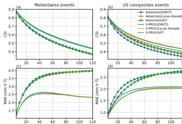
Determination of the advection field by optical flow is a key component of any extrapolation-based nowcasting system. Pysteps allows to easily analyze the impact of the optical flow method and also scale filtering on the forecast skill. More-over, the three methods currently available in themotion module constitute an ideal testbed as they cover three very distinct approaches; see the references in Sect. 2.1 for de-tails. The experiments were done by using the MeteoSwiss and US precipitation events described in Tables 8 and 9.
simi-Figure 11.Comparison of forecast skill using different optical flow and extrapolation methods. Panels(a)and(c)show the averaged CSI and MAE for the MeteoSwiss events listed in Table 8, while(b)and(d)show the same results but for the US events listed in Table 9. The CSI is computed using a 0.1 mm h−1threshold.
lar behavior is observed for the US events (Fig. 11b and 11d) but with a∼20 % the reduction in MAE after 2 h.
On the other hand, no significant differences can be ob-served between different optical flow methods (less than 2 %), with DARTS performing slightly worse than the other methods. This is possibly explained by the fact that, with the default configuration, DARTS produces only a large-scale approximation of the advection field.
Figure 12 shows advection fields obtained using different optical flow methods for a selected case (US, 11 April 2013 at 08:00 UTC). Lucas–Kanade and VET produce smooth fields that are remarkably similar, particularly close to the precipitation areas (Fig. 12a and b). Within precipitation ar-eas, DARTS produces similar motion fields to the other two methods, but outside precipitation the fields are considerably different.
We also measured the computation times of different op-tical flow methods in the MeteoSwiss and FMI domains, and the results are shown in Table 6. The experiments were done using an Intel Xeon E5645 CPU with 12 cores running at 2.4 GHz with parallelization enabled in the optical flow methods. The results reflect the fact that the Fourier space and local methods (DARTS and Lucas–Kanade) have sig-nificantly lower computational requirements than variational methods (VET), which are however still within the needs of a real-time operational system. Thus, our conclusion from the results shown in Fig. 11 and Table 6 is that the choice of the optical flow method plays a less significant role, while
Table 6.Average computation times of different optical flow meth-ods in the MeteoSwiss and FMI domains (seconds). Domain sizes are given in parentheses.
12 cores
Method MeteoSwiss FMI
(710×640) (760×1226)
DARTS 4.02 4.07
Lucas–Kanade 2.02 4.29
VET 13.73 28.98
1 core
Method MeteoSwiss FMI
(710×640) (760×1226)
DARTS 4.27 4.78
Lucas–Kanade 2.07 4.46
VET 41.65 85.14
nowcast errors are more clearly determined by the dynamic scaling properties of precipitation as highlighted by the large impact of scale filtering on the forecast skill.
5.2 Ensemble size
Figure 12. Comparison of advection fields obtained by differ-ent optical flow methods for a selected precipitation evdiffer-ent: US, 11 April 2013 at 08:00 UTC.
the optimal number, the skill of the nowcasts with different intensity thresholds and ensemble sizes was evaluated by us-ing two metrics. These are the area under the ROC curve and the outlier percentage (OP). The results are shown in Figs. 13 and 14.
Figure 13 shows that the choice of the ensemble size plays a significant role, which is particularly true when nowcasts of higher precipitation intensities are desired. Figure 13a shows that for n=6, the ROC area falls below 0.85 after 2 h, while it is close to 0.9 whennis increased to 48. How-ever, there is only marginal improvement whennis increased from 24 to 48, which suggests that 24 members are suffi-cient when nowcasts of precipitation/no precipitation are de-sired with low-intensity thresholds (e.g., 0.1 mm h−1). On the other hand, Fig. 13b shows that when the threshold is
in-Figure 13.ROC areas for(a)0.1 mm h−1and(b)5 mm h−1 thresh-olds with different ensemble sizes as a function of lead time during the MeteoSwiss events listed in Table 8.
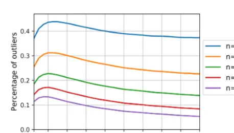
Figure 14.Outlier percentages (OPs) with different ensemble sizes as a function of lead time during the MeteoSwiss events listed in Table 8.
creased to 5 mm h−1, a significant improvement can be ex-pected when increasingnfrom 48 to 96 or even over 100.
Figure 15.Averaged computation times of pysteps nowcast ensem-bles with different ensemble sizes and number of parallel threads for the(a)MeteoSwiss and(b)FMI domain. The grid sizes for the domains are 710×640 and 760×1226 pixels, respectively. The 1 h nowcasts with 12 time steps of 5 min were computed for both do-mains. The computation times include only the ensemble computa-tion, excluding the optical flow, the initialization of the model and writing the results to disk.
of OP on the lead time. The highest OP can be observed at 20 min, and after 3 h it is up to 50 % smaller.
We also analyzed the computation times needed to gener-ate nowcast ensembles. In a real-time setting, it is essential to know how many ensemble members can be produced be-fore the arrival of the next input radar rainfall image (usually every 5 min). To this end, 1 h nowcasts were computed with different ensemble sizes and number of parallel threads us-ing the FMI and MeteoSwiss data listed in Tables 7 and 8, respectively.
The results of the above experiments are shown in Fig. 15. Figure 15a shows that for the input grid of 710×640 pixels used in the MeteoSwiss domain, it is possible to generate 1 h nowcast ensembles of up to 48 members in less than 2 min using a server with 12 processor cores.
The results for the larger FMI domain with grid size of 760×1226 pixels are shown in Fig. 15b. Compared to the MeteoSwiss domain, the height of the grid is doubled, which also doubles the computation time (the computational
com-plexity increases quadratically with respect to grid size). Nevertheless, using 12 processor cores, the computation time of a 48-member ensemble still remains below 2 min.
In addition, Fig. 15a and b show the effectiveness of the parallelization scheme implemented in pysteps. That is, when plotted in logarithmic scale, the computation time de-creases approximately linearly with respect to the number of threads (i.e., the computation time is halved when the num-ber of threads is multiplied by 2).
5.3 Localization
This experiment investigates the impact of localization on the nowcast quality. In this context, localization means restrict-ing the nowcastrestrict-ing model into small subdomains instead of applying it the whole domain assuming spatial homogeneity of the precipitation field, as in the earlier STEPS implemen-tations (e.g., Bowler et al., 2006). To this end, the short-space approach presented in Nerini et al. (2017) for stochastic noise generation is generalized to the whole nowcasting system (see modulenowcasts.sseps). Adapting the approach described in Sideris et al. (2018), the parameter estimation and the nowcasting model are implemented in a moving win-dow of predetermined size. The localization is applied to the cascade decomposition, the autoregressive process (5), the non-parametric Fourier filter (10) and the probability match-ing (15).
The impact of localization is assessed in terms of rank his-tograms and reliability diagrams (threshold of 1.0 mm h−1) for a 30 min lead time (Fig. 16). The localization shows pos-itive effects in the ensemble spread, which improves both in terms of reliability and conditional bias, although we also ob-serve a slight decrease of sharpness. This is reflected in the rank histograms, which tend to get flatter as the localization window gets smaller. This seems to be mainly driven by a reduction in the proportion of observations lying above the ensemble, which reduces from approximately 13 % to 8 %. 5.4 Cascade decomposition
lev-Figure 16.Effect of localization in terms of(a)rank histograms and(b)reliability diagrams computed for the 30 min lead time and 1 mm h−1during the MeteoSwiss events (Table 8). The localization window was reduced from the full domain (710 km) to three differ-ent local scales (360, 180 and 90 km).
els, respectively. The objective is to analyze the realism of the temporal evolution, not whether the AR is an appropri-ate model of the forecast error as in Sect. 4.6. In practice, this implies comparing the theoretical ACFs of forecast and observed fields as follows: (1) generate nowcasts with either an eight-level or one-level cascade, (2) transform the fore-cast fields into the Lagrangian frame (by using the same mo-tion field estimated at start time), (3) decompose the forecast fields into a six-level cascade, (4) estimate the AR(2) param-eters at each scale, (5) derive the full temporal ACF (see also Fig. 10) and (6) integrate the ACF to estimate the precipita-tion lifetime. The procedure is repeated for each forecast lead time up to 2 h and also for the corresponding observations.
Figure 17.Verification of dynamic scaling properties of stochas-tic nowcasts generated with one and eight cascade levels. All Me-teoSwiss events were analyzed, but nowcasts were run only ev-ery 4 h.
Figure 17 shows the average lifetime for all the Me-teoSwiss events plotted against spatial wavelength (in log– log scale). As expected, the model with eight cascade levels reproduces well the dynamic scaling properties, especially at small wavelengths. However, there is some degree of over-estimation of the lifetime at large wavelengths compared to the observations. One possibility would be to adjust the AR parameters to obtain faster decorrelation, and thus a shorter lifetime, at such scales.
The model without cascade decomposition compen-sates for the overestimation of persistence at large lengths but strongly overestimates the one of small wave-lengths. Hence, the evolution of convective cells in the stochastic nowcast is too slow compared with reality. This could be checked visually by looking at the ani-mations of stochastic realizations with and without de-composition (*_stoch_*.gif in https://github.com/pySTEPS/ pysteps-publication/tree/master/animations, last access: 23 September 2019).
Another approach to understand the impact of the cascade decomposition is to analyze the filtering properties of the en-semble mean forecast (e.g., Surcel et al., 2014). Figure 18 illustrates the evolution of the ensemble mean forecast spec-tra with eight and one cascade levels, respectively. When using the cascade decomposition the process of ensemble averaging leads to a loss of power at small spatial wave-lengths, in agreement with the expected loss of predictability (see Sect. 4.5). Instead, the model with one cascade level is not able to filter out the unpredictable features. As a conse-quence, it may not be able to adequately characterize the loss of predictability (and uncertainty) at different spatial scales.
Figure 18.Spatial structure analysis of the ensemble mean forecast using(a)eight cascade levels and(b)one cascade level. Both experiments have an ensemble size of 24 members. MeteoSwiss event no. 3 was used.
Figure 19. Ensemble and probabilistic verification of the cascade experiments for all the MeteoSwiss cases with and without cascade decomposition, and with and without masking.(a)Rank histograms at 60 min,(b)spread–error relationship,(c, d)reliability diagrams at 60 min for probability of rain exceeding 0.1 and 1 mm h−1, respectively.
estimations on using the incremental precipitation mask is also included.
The rank histograms behave differently depending on the chosen forecast settings (Fig. 19a). The two models without decomposition denote a clear overdispersion with a charac-teristic dome-shape in the bin range 13–22, especially for the setting with one level and no mask. Instead, the models with eight levels display a flat histogram, except for the very last bin, which contains the frequency of observations exceeding all the ensemble members (misses). As shown in Fig. 14, this
underdispersion can be reduced by increasing the ensemble size. The last bin is also quite sensitive to using the mask, which prevents the ensemble to capture the uncertainty asso-ciated to precipitation initiation far from the main precipita-tion body.
Figure 20.Comparison of a member of 5 min rainfall ensemble for(b)+30 min,(c)+60 min and(d)+120 min nowcasts initialized with (a)radar-based rainfall analysis from the Australian radar network valid at 06:05 UTC on 1 January 2019 on a 512×512 pixel grid (256×
256 km) (event no. 2 in Table 10).
Figure 21.Comparison of a member of 5 min rainfall ensemble for(b)+30 min,(c)+60 min and(d)+120 min nowcasts initialized with (a) radar-based rainfall analysis from the Australian radar network valid at 07:15 UTC on 8 February 2019 on a 512×512 pixel grid (256×256 km) (event no. 1 in Table 10).
be noticed that the one-level models do not show the same overdispersion that was observed on the rank histograms.
Finally, the reliability diagrams of Fig. 19c–d demonstrate a very good reliability for all forecast settings, although the forecast probabilities of the models with one level are slightly lower than the observed frequencies. In addition, the eight-level model has better sharpness, i.e., a larger proportion of high forecast probabilities (>0.9).
6 Nowcasting the extremes: two severe-weather case studies from Australia
An example of applying the pysteps library in order to fore-cast rainfall fields for tropical cyclone Penny and severe con-vection in Sydney (Australia) is shown in Figs. 20 and 21, respectively. The ability of pysteps to estimate diverse advec-tion patterns from observed data is quite clear in these exam-ples, with the tropical cyclone case showing a clear clock-wise rotational pattern, while the severe convection shows an almost even easterly flow pattern across the whole domain. Tropical cyclone nowcasts preserve the original cyclonic pat-tern up to 60 min ahead but some distortions are induced for longer lead times due to convergence and divergence. The severe convection case has a simpler advection pattern that
helps to preserve the general structure of the observed rain-fall fields beyond 60 min. Additional data sources such as satellite or NWP forecasts may help to estimate future advec-tion velocities and reduce potential anomalies for longer lead times. It is important to note, however, that post-processing of nowcasts (see Sect. 2.8) ensures that the forecast rainfall fields have the same statistical properties with the observed ones in both case studies.
6.1 Neighborhood verification
Figures 22 and 23 show examples of FSS results calculated by pysteps for different forecast times for both Australian case studies.
Figure 22.Comparison of fractions skill score (FSS) values for(a)+10 min,(b)+30 min and(c)+60 min nowcasts rainfall ensembles for tropical cyclone Penny (event no. 1 in Table 10). FSS values were calculated comparing the ensemble mean for each lead time with observations.
Figure 23.Same as Fig. 22 but for the severe convection case study (event no. 2 in Table 10).
the relatively low number of high-intensity samples in these events.
On the other hand, the severe convection case displays a stronger decay of skill when spatial scale is reduced, prob-ably due to the presence of sharp spatial gradients and iso-lated convective cells. This said, it is interesting to note how for the higher intensities and large spatial scales the FSS val-ues do not decay as heavily as seen in the other case study. This difference could be a consequence of having more high-intensity values in the severe convection event.
6.2 Lifetime of rainfall fields per spatial scale
To compare the behavior of the AR(2) model for these two case studies, temporal auto-correlation functions for each spatial scale were calculated using Eq. (7) and then inte-grated to estimate the precipitation lifetimes for each scale and runtime. Figure 24 summarizes the precipitation lifetime results for each case study. Overall, a more diverse set of spatial and temporal patterns observed during the severe con-vection event makes interquartile ranges of precipitation life-times larger for this case study for all scales. In comparison,
similar organized patterns were present during most of the duration of the tropical cyclone event and therefore precipi-tation lifetime values have a narrower range. Smaller scales seem to have similar average lifetime values for both cases with no strong temporal variations within the events. For the larger scales, however, precipitation lifetime values for trop-ical cyclone event are greater than severe convection ones, again as a consequence of large-scale organized patterns ob-served in this event.
Table 7.Precipitation events in Finland (FMI). The duration of each event is 12 h.
No. Date Start time Description (UTC)
1 8 Jun 2016 13:00 A low-pressure system over northern Finland causes frontal rain associated with a warm front and frontal rain and convective cells associated with a cold front. The system moves eastward with precipitation areas rotating around its center.
2 15 Jul 2016 12:00 Frontal precipitation approaches measurement area from the south.
3 28 Sep 2016 09:00 Frontal precipitation intermixed with convection, some scattered convective cells.
4 22 Feb 2017 22:00 Widespread heavy frontal precipitation associated with a low-pressure system traversing over southern Finland.
5 8 Jun 2017 04:00 Narrow and slowly moving precipitation band.
6 14 Jul 2017 01:00 Precipitation starts out as a narrow precipitation band with some scattered convective cells and later evolves into predominantly convective precipitation.
7 4 Aug 2017 11:00 Frontal rain associated with a warm front and some convective activity. 8 12 Sep 2017 03:00 Frontal precipitation moves northward and slightly rotates.
9 12 Aug 2018 05:00 Frontal precipitation intermixed with convection. Some convective activity, which rotates. Convective activity increases noticeably in a few hours.
10 29 Sep 2018 16:00 Frontal precipitation moves eastward and is followed by convective activity. New convective cells are continuously generated at the northern coast of Estonia after the frontal precipitation has passed.
Table 8.Precipitation events in Switzerland (MeteoSwiss). The duration of each event is 12 h.
No. Date Start time Description (UTC)
1 16 Apr 2016 18:00 Prefrontal precipitation induced by a low-pressure system over the North Sea. Lines of convection develop over western Switzerland.
2 11 Jul 2016 13:00 An approaching cold front causes widespread convective activity in a southwesterly flow. 3 31 Jan 2017 10:00 A strong northwesterly flow causes orographic blocking on the northern slopes of the Alps
resulting in widespread precipitation.
4 14 Jun 2017 13:00 Fairly uniform pressure distribution across central Europe; scattered convection develops during the afternoon.
5 24 Jun 2017 22:00 Prefrontal activity with intense thunderstorms south of the Alps. Measured peak intensity reached 33.5 mm in 10 min and presence of large-size hailstones (3–5 cm) was observed. 6 27 Jun 2017 20:00 A frontal passage during the night induces organized convection over the domain and important
prefrontal convective activity on the southern side of the Alps.
7 19 Jul 2017 13:00 In a southwesterly flow, development of large convective cells over central Switzerland. 8 21 Jul 2017 13:00 Flat pressure distribution across central Europe, southwesterly flow associated to a low over the
British Islands. Clusters of intense thunderstorms develop over western Switzerland. 9 29 Jul 2017 13:00 Southwesterly flow connected to large depression over British Islands. Large clusters of
convection develop south of the Alps.
10 31 Aug 2017 14:00 Strong southwesterly flow over the Alps associated to a cold front. Important lines of stationary convection affect the southern Alps, while more stratiform precipitation occurs in the west and north of Switzerland.
7 Conclusions
Pysteps is an open-source library for radar-based probabilis-tic precipitation nowcasting written in Python. It represents a community-based initiative that aims at connecting now-casting scientists by sharing code, methods, ideas and results and also providing an easy-to-use tool for operational appli-cations.
Pysteps implements the main components of an ensem-ble precipitation nowcasting system. These are input/output, optical flow and extrapolation routines, time series methods for modeling the temporal evolution of precipitation fields, stochastic noise generation in space and time, visualization and forecast verification.
Table 9.Precipitation events from the US. The duration of each event is 12 h.
No. Date Start time Description (UTC)
1 16 Apr 2011 08:00 Large extratropical cyclone. The low-pressure center was located over the Great Lakes with a strong cold front extending south.
2 15 Nov 2011 23:00 Frontal precipitation associated with a stationary front in the southeastern US.
3 4 Apr 2013 18:00 Two widespread precipitation systems produced by two cyclonic systems over the US, located in the northwest and southeast of the US.
4 11 Apr 2013 00:00 Midlatitude cyclone over the eastern US with the eastern line of precipitation caused by a cold front extending in the south–north direction from eastern Texas to central Missouri and in the west–east direction from Missouri to the south of the state of New York.
5 18 May 2013 06:00 Mesoscale convective systems (MCSs) located in northern and southeastern US.
6 27 May 2017 00:00 MCSs developed over central and northwestern US, along with a cyclonic precipitation system located in southeastern Canada.
Table 10.Precipitation events from Australia (BoM). The duration of each event is 12 h.
No. Date Start time Description (UTC)
1 1 Jan 2019 00:00 Tropical cyclone Penny moving from the Gulf of Carpentaria and making landfall on the western Cape York Peninsula coastline just south of Weipa C-band Doppler radar. 2 8 Feb 2019 05:00 Severe convection activity observed by the S-band polarimetric radar of Terry Hills near
Sydney. Convective cells are continuously generated inland New South Wales and intensifying as they move east. This event produced thunderstorms, heavy rainfall and flash flooding in the city of Parramatta and western Sydney suburbs.
Figure 24.Distribution of precipitation lifetime values for each spa-tial scale during tropical cyclone (event no. 1 in Table 10) and severe convection (event no. 2 in Table 10) case studies.
The library has a modular design so that developers can eas-ily interchange components and embed them into other soft-ware packages.
In this paper, we briefly explained the framework of prob-abilistic precipitation nowcasting and how such nowcasts can be produced using pysteps. The potential of pysteps was demonstrated using radar composite images from Fin-land (FMI), SwitzerFin-land (MeteoSwiss), the United States and Australia (BoM). Finally, we performed experiments where the quality of pysteps nowcasts and computational perfor-mance were evaluated with different configurations. This brought us to the following conclusions:
1. Probabilistic precipitation nowcasts computed with pys-teps have good reliability that, however, decreases for increasing rainfall intensity thresholds and lead time. Using the MeteoSwiss data, it was shown that for the 0.1 mm h−1 threshold, reliable nowcasts with poten-tially useful skill can be obtained up to 3 h. When the threshold was increased to 5 mm h−1, useful nowcasts could still be obtained up to 45 min (Figs. 5 and 6). 2. Rank histograms show that the ensemble spread has