Nonparametric Estimation of Probability Density Functions of
Random Persistence Diagrams
Vasileios Maroulas [email protected]
Department of Mathematics University of Tennessee Knoxville, TN 37996, USA
Joshua L Mike [email protected]
Computational Mathematics, Science, and Engineering Department Michigan State University
East Lansing, MI 48823, USA
Christopher Oballe [email protected]
Department of Mathematics University of Tennessee Knoxville, TN 37996, USA
Editor:Boaz Nadler
Abstract
Topological data analysis refers to a broad set of techniques that are used to make inferences about the shape of data. A popular topological summary is the persistence diagram. Through the language of random sets, we describe a notion of global probability density function for persistence diagrams that fully characterizes their behavior and in part provides a noise likelihood model. Our approach encapsulates the number of topological features and considers the appearance or disappearance of those near the diagonal in a stable fashion. In particular, the structure of our kernel individually tracks long persistence features, while considering those near the diagonal as a collective unit. The choice to describe short persistence features as a group reduces computation time while simultaneously retaining accuracy. Indeed, we prove that the associated kernel density estimate converges to the true distribution as the number of persistence diagrams increases and the bandwidth shrinks accordingly. We also establish the convergence of the mean absolute deviation estimate, defined according to the bottleneck metric. Lastly, examples of kernel density estimation are presented for typical underlying datasets as well as for virtual electroencephalographic data related to cognition.
Keywords: Topological Data Analysis; Persistence Homology; Finite Set Statistics; Global Dis-tribution of Persistence Diagrams; Kernel Density Estimation; EEG Signals
1. Introduction
Topological data analysis (TDA) encapsulates a range of data analysis methods that investigate the topological structure of a dataset (Edelsbrunner and Harer, 2010). One such method, persistent homology, describes the geometric structure of a given dataset and summarizes this information as a persistence diagram. TDA, and in particular persistence diagrams, have been employed in several studies with topics ranging from classification and clustering (Venkataraman et al., 2016; Adcock et al., 2016; Pereira and de Mello, 2015; Marchese and Maroulas, 2018) to the analysis of dynamical
c
systems (Perea and Harer, 2015; Sgouralis et al., 2017; Guillemard and Iske, 2011; Seversky et al., 2016) and complex systems such as sensor networks (De Silva and Ghrist, 2007; Xia et al., 2015; Bendich et al., 2016). In this work, we establish the probability density function (pdf) for a random persistence diagram.
Persistence diagrams offer a topological summary for a collection of d-dimensional data, say {xi} ⊂ Rd, which focuses on the global geometric structure of the data. A persistence diagram is a multiset of homological features {(bi, di, ki)}, each representing a ki-dimensional hole which
appears at scalebi ∈R+ and is filled at scale di ∈(bi,∞). In general, the dataset arises from any metric space, though restricting to {xi} ⊂Rd guarantees ki ∈ {0, ...,d−1}. For example, if the data form a time series trajectoryxi =f(ti), the associated persistence diagram describes
multista-bility through a corresponding number of persistent 0-dimensional features or periodicity through a single persistent 1-dimensional feature. In a typical persistence diagram, few features exhibit long persistence (range of scales di−bi), and such features describe important topological
characteris-tics of the underlying dataset. Moreover, persistent features are stable under perturbation of the underlying dataset (Cohen-Steiner et al., 2010).
Persistence diagrams have recently seen intense active research, including significant successful efforts toward facilitating previously challenging computations with them; these efforts impact evaluation of Wasserstein distance in (Kerber et al., 2016) and the creation of persistence diagrams with packages such as Dionysus (Fasy et al., 2015) and Ripser (Bauer, 2015) which take advantage of certain properties of simplicial complexes (Chen and Kerber, 2011). Recently, various approaches have defined specific summary statistics such as center and variance (Bobrowski et al., 2014; Mileyko et al., 2011; Turner et al., 2014; Marchese and Maroulas, 2018), birth and death estimates (Emmett et al., 2014), and confidence sets (Fasy et al., 2014). While the aforementioned studies focus on valuable specific summaries, here we view a distribution of persistence diagrams in a global sense via a nonparametric method to estimate its density function.
non-parametric means. Kernel density estimation is a well known nonnon-parametric technique for random vectors in Rd (Scott, 2015) which relies on convolution with a smooth kernel.
There has been extensive work to devise various maps from persistence diagrams into Hilbert spaces, especially Reproducing Kernel Hilbert Spaces (RKHS). For example, (Adams et al., 2017) discretizes persistence diagrams via bins, yielding vectors in a high dimensional Euclidean space; the authors in (Chazal and Divol, 2018) introduce a novel bandwidth selection procedure for this particular vectorization based on cross-validation. The persistence landscapes of (Bubenik, 2015) reinterpret the space of persistence diagrams within a function-based vector space. The works (Reininghaus et al., 2014) and (Kusano et al., 2016) define kernels between persistence diagrams in a RKHS. By mapping into a Hilbert space, these studies allow the application of machine learning methods such as principal component analysis, random forest, support vector machine, and more. The universality of such a kernel is investigated in (Kwitt et al., 2015); this property induces a metric on distributions of persistence diagrams (by comparing means in the RKHS), as (Kwitt et al., 2015) demonstrates with a two-sample hypothesis test. In a similar vein, (Adler et al., 2017) uses Gibbs distributions in order to replicate similar persistence diagrams, e.g. for use in MCMC type sampling.
By mapping into a Hilbert space, the preceding approaches kernelize persistence diagrams for express application in typical machine learning methodology. In a similar vein, the studies (Bo-browski et al., 2014) and (Fasy et al., 2014) work with kernel density estimation on the underlying data to estimate a target diagram as the number of underlying datapoints goes to infinity. In both cases, the target diagram is directly associated to the probability density function (pdf) of the underlying data via the superlevel sets of the pdf. The first work constructs an estimator for the target diagram, while the second defines a confidence set. In either case, kernel density estimation is used to approximate the pdf of the underlying datapoints, assuming the data are independent and identically distributed (i.i.d.). In complementary fashion, our work considers a new kernel density defined on a completely different space: the space of persistence diagrams.
Since persistence diagrams lack a vector space structure, we must smooth without convolution. Instead, we treat persistence diagrams as random multisets and provide a noise model for persistence diagrams which ascribes a great level of uncertainty near the diagonal. The theory of random sets is an interpretation of point processes which provides the tools necessary to describe the global pdf of the noise model as a kernel density centered at a particular persistence diagram. Instead of a transformed collection or a center diagram, the output of our method is an estimate of a probability density function (pdf) of a random persistence diagram. Access to a persistence diagram pdf facilitates definition and application of new statistical techniques in this context such as hypothesis testing, utilization of Bayesian priors, or likelihood based methods, e.g. see (Maroulas et al., 2019). The proposed kernel density is centered at a persistence diagram and describes each feature as having either short or long persistence; by treating each long-persistence point individually and short persistence points collectively, the kernel density strikes a careful balance between accuracy and computation time. Our method also enables expedient sampling of new persistence diagrams from the kernel density estimate. In contrast to previous methodologies, our kernel density estimate has the potential to describe high probability features in a random persistence diagram, even if these features have brief persistence. Such features are typically indicative of the geometric structure, e.g., curvature, of the dataset rather than its topology.
The homological features (bi, di, ki) in a persistence diagram come without an ordering and
dataset. Thus, any notion of density must be (i) invariant to the ordering of features and (ii) account for variability in their cardinality. Indeed, the approach used to analyze a collection of persistence diagrams in (Bendich et al., 2016) is a good step toward understanding a random per-sistence diagram, but requires a choice of order and considers only a fixed number of features and is therefore unsuitable for creating probability densities. In this work, we offer a kernel density with the desirable properties (i) and (ii), which also calls attention to the persistence of each feature. A typical persistence diagram has many features with brief persistence and few with moderate or longer persistence; consequently, our kernel density groups features with short persistence together in order to combat the curse of dimensionality. Indeed, the kernel density still considers features of short persistence, but simplifies their treatment in order to facilitate computation. The kernel density is defined on a pertinent space of finite random sets which is equipped to describe pdfs for random persistence diagrams generated from associated data with bounded cardinality of topolog-ical features. In this sense, our kernel density provides estimation of the distribution of persistence diagrams which in turn describes the geometry of the random underlying dataset. The requirement of bounded feature cardinality is trivially satisfied for datasets with bounded cardinality, which is reasonable for application and theory. Indeed, the creation of a persistence diagram from an infi-nite collection of data is often nonsensical (e.g., for anything with unbounded noise), and a scaling limit should be considered instead; For example, this problem can be approached via the studies (Bobrowski et al., 2014) and (Fasy et al., 2014).
The overallcontribution of this article is listed below.
1. A probabilistic framework for defining distributions of random persistence diagrams.
2. A novel kernel density estimator centered at persistence diagrams, which in part provides a noise likelihood model, and its convergence to the true distribution as the number of persis-tence diagrams goes to infinity.
3. A new dispersion statistic for persistence diagrams, the mean absolute bottleneck deviation (MAD) and the convergence of the sample MAD computed with our kernel density estimator.
4. Applications of the kernel density estimator to analyze data data arising from a neuroscience problem related to cognition.
problem (Example 4). Finally, we end with conclusions and discussion in Section 6. Further examples of KDE convergence and the proofs of auxiliary propositions and lemmas are given in the supplementary materials.
2. Topological Data Analysis Background
The topological background discussed here builds toward the definition of persistence diagrams, the pertinent objects in this work. We begin by briefly discussing simplicial complexes and homology, an algebraic descriptor for coarse shape in topological spaces. In turn, persistent homology, and its summary, persistence diagrams, are techniques for bringing the power and convenience of homology to describe subspace filtrations of topological spaces. The reader should refer to (Edelsbrunner and Harer, 2010), for example, for a rigorous treatment of persistent homology. We first consider topological spaces of discernible dimension, called manifolds.
Definition 1 A topological space X is called ak-dimensional manifold if every point x∈X has a neighborhood which is homeomorphic to an open neighborhood in k-dimensional Euclidean space.
We generalize the fixed-dimension notion of a manifold in order to define simplicial homology for simplicial complexes. We then discuss the ˇCech construction which is used to associate simplicial complexes to datasets.
Definition 2 Ak-simplex is a collection ofk+1linearly independent vertices along with all convex combinations of these vertices: (v0, ..., vk) =
n Pk
i=0αivi:Pki=0αi = 1 and αi ≥0∀i
o
. Topologi-cally, a k-simplex is treated as a k-dimensional manifold (with boundary). An oriented simplex is typically described by a list of its vertices, such as (v0, v1, v2). The faces of a simplex consist of all
the simplices built from a subset of its vertex set; for example, the edge (v1, v2) and vertex (v2) are
both faces of the triangle (v0, v1, v2).
Definition 3 A simplicial complex K is a collection of simplices wherein (i) ifσ ∈ K, then all its faces are also inK, and (ii) the intersection of any pair of simplices in K is another simplex inK.
A simplicial complex is realized by the union of all its simplices; some examples are shown in Fig. 1. Conditions (i) and (ii) in Def. 3 establish a unique topology on the realization of a simplicial complex which restricts to the subspace topology on each open simplex. For finite simplicial complexes realized inRd, this topology is also consistent with the Euclidean subspace topology.
Given a simplicial complex, we are interested in describing its global topology and local geome-try through homological features. For our purposes, it suffices to definek−dimensional homological features of simplicial complexes as k−dimensional holes, so that, for example, 0−dimensional ho-mological features are connected components, 1−dimensional homological features are loops, and 2−dimensional homological features are voids.
We wish to extend the notion of homology for a discrete set of data x = {xi}Ni=1 within a metric space (X, dX). Treating the set itself as a simplicial complex, its homology yields only the
cardinality of the data points. So, we use the metric to obtain more information. Here we denote byB(x0, r0) a metric ball centered atx0 of radiusr0. Fix a radiusr >0 and consider the collection of neighborhoodsU ={Ui}={B(xi, r)}along with its unionUr =∪iB(xi, r). The filtration of sets
Figure 1: The neighborhood space and ˇCech complex of matching radius plotted at three different radii. Yellow indicates a triangle while orange indicates a tetrahedron. This family of simplicial complexes is the filtration used to compute and define persistent homology.
scales. To make homology computations more tractable forUr, we instead consider the associated
nerve complexes.
Definition 4 The nerve N(U) of a collection of open sets U is the simplicial complex where a
k-simplex (vi0, ..., vik) is in N(U) if and only if ∩k
j=0Uij 6= ∅. The nerve of the neighborhoods
U ={B(xi, r)}is called the ˇCech complex on the data{xi}at radiusr and is denoted by ˇCech(x, r).
Examples of the ˇCech complex for the same data at different radii are depicted in Fig. 1, where they are superimposed with the associated neighborhood space. Any nerve complex trivially satisfies the requirements for a simplicial complex (Edelsbrunner and Harer, 2010). Moreover, the nerve theorem states that the nerve and union of a collection of convex sets have similar topology (they are homotopy equivalent) (Hatcher, 2002); specifically, the ˇCech complex and neighborhood space U have identical homology for any given radius.
A priori, it is unclear which choice of scale (radius), best describes the data; and oftentimes different scales reveal different information. Thus, to investigate the topology of our data, we consider the appearance and disappearance of homological features at growing scale. This multiscale viewpoint, called persistent homology, is introduced in (Edelsbrunner et al., 2002) and yields a topological summary of the data called a persistence diagram. This is possible because we have a growing filtration of complexes, so each complex is included in the next (see Fig. 1). These inclusion maps induce maps at the level of homology groups. These induced maps are referred to here as the persistence maps, and take features to features or to zero (Cohen-Steiner et al., 2007). Thus, each feature is tracked by how far the persistence maps preserve it. In turn, tracking features is boiled down to a very specific algorithm for obtaining the birth and death radii for each homological feature (e.g., see (Edelsbrunner and Harer, 2010)). Features which persist over a large range of scale are typically considered more important, and their presence is stable under small perturbations of the underlying data (Cohen-Steiner et al., 2010).
Persistent homology yields a multiset of homological features, each born at a scale bi, lasting
until its death scale di, with degree of homology ki; in short, it yields a persistence diagram
D = {ξi}Mi=1 = {(bi, di, ki)}Mi=1. We interpret the birth-death values as coordinate points with degree of homology as labels. For clarity and simplicity, we ignore any features with death value
di=∞, since these features are generally a characteristic of the ambient space. In particular, one
Specifically, for data inRd, we consider each feature as an element of
W0:d−1 =W × {0, ...,d−1}, (2.1)
where W =
(b, d)∈R2 :d > b≥0 is the infinite wedge. As a topological space, the d-fold multiwedge W0:d−1 is treated as d-disconnected copies of W, where W has the Euclidean metric and topology.
It is desirable to define a metric between persistence diagrams with which to measure topologi-cal similarity. In TDA, Hausdorff distance is typitopologi-cally used to compare underlying datasets, while the bottleneck distance (Def. 5) is used to compare their associated persistence diagrams (Fasy et al., 2014; Munch, 2017). A distance that accounts for cardinality differences between persis-tence diagrams was introduced in (Marchese and Maroulas, 2018) and its stability with respect to perturbations in the underlying point cloud was proved in (Maroulas et al., 2018).
Definition 5 The bottleneck distance between two persistence diagrams D1 andD2 is given by
W∞(D1, D2) = min
γ maxx∈D1kx−γ(x)k∞. (2.2)
where γ ranges over all possible bijections between D1 and D2 which match in degree of homology.
The diagonal{b=d} is included in both persistence diagrams with infinite multiplicity so that any feature may be matched to the diagonal.
Remark 6 Due to the unstable presence of features near the diagonal, typical metrics on persis-tence diagrams such as the bottleneck distance treat the diagonal as part of every persispersis-tence diagram (Mileyko et al., 2011) in order to achieve stability with respect to Hausdorff perturbations of the un-derlying dataset (Cohen-Steiner et al., 2007). Morally, one considers the diagonal as representing vacuous features which are born and die simultaneously. For convenient computation, the definition of bottleneck distance can be applied to each degree of homology separately.
3. Random Persistence Diagrams
In this section we establish background to make the notion of probability density for a random per-sistence diagram explicit and well-defined. A perper-sistence diagram changes its feature cardinality under small perturbation of the underlying dataset, and these features have no intrinsic order. Con-sequently, we cannot treat persistence diagrams as elements of a vector space. Instead, we consider a random persistence diagramDas a random multiset of featuresD={ξi} ⊂ W0:d−1 in the multi-wedge defined in Eq. (2.1). For underlying datasets sampled fromRdwith bounded cardinality, the affiliated ˇCech persistence diagrams also have bounded feature cardinality and degree of homology. Thus, we assume that the cardinality of a random persistence diagram is bounded above by some value|D| ≤M ∈N, and so consider the spaceC≤M(W0:d−1) ={Dmultiset in W0:d−1 :|D| ≤M}. We view C≤M(W0:d−1) through a list of functions hN which each map the appropriate
dimen-sion of Euclidean space into its corresponding cardinality component,CN(W0:d−1). This viewpoint facilitates the definition of probability densities.
Definition 7 For each N ∈ {0, ..., M}, consider the space of N topological features, denoted
CN(W0:d−1) ={D multiset inW0:d−1 :|D|=N}, and the associated maphN :W0:Nd−1→ CN(W0:d−1)
defined by
The maphN creates equivalence classes onW0:Nd−1 according to the action of the permutations ΠN;
specifically,[Z] = [(ξ1, ..., ξN)]hN =
ξπ(1), ..., ξπ(N)
:π ∈ΠN for eachZ = (ξ1, ..., ξN)∈ W0:Nd−1.
These equivalence classes yield the space
WN
0:d−1/ΠN =
n
[ξ]hN :ξ∈ WN
0:d−1
o
, (3.2)
equipped with the quotient topology. The topology onC≤M(W0:d−1)is defined so that eachhN lifts to
a homeomorphism betweenWN
0:d−1/ΠN andCN(W0:d−1), and we writeW0:dN −1/ΠN ∼=CN(W0:d−1). With a topology in hand, one can define probability measures on the associated Borelσ-algebra. Thus, we define a random persistence diagram D to be a random element distributed according to some probability measure on C≤M(W0:d−1) for a fixed maximal cardinalityM ∈N. We denote associated probabilities by P[·] and expected values byE[·]. Since W0:Nd−1/ΠN ∼=CN(W0:d−1), we work toward defining probability densities on the collection of Euclidean spaces ∪M
N=0W0:Nd−1. Definition 8 For a given random persistence diagram D and any Borel subset A of W0:d−1, the
belief function βD is defined as
βD(A) =P[D⊂A]. (3.3)
Since A is a Borel subset of W0:d−1, the collection OA = {D∈ C≤M(W0:d−1) :D⊂A} is the quotient of ∪M
N=0AN ⊂ ∪MN=0W0:dN −1 under hN; moreover, AN is clearly Borel in the Euclidean
topology of∪M
N=0W0:Nd−1. Therefore, sincehN induces a homeomorphism (see definition 7),OAis a
Borel subset ofC≤M(W0:d−1). The belief function of a random persistence diagram is similar to the joint cumulative distribution function for a random vector, in particular by yielding a probability density function through Radon-Nikod´ym type derivatives.
Definition 9 Fix φdefined on Borel subsets of C≤M(W0:d−1) into R. For an element ξ∈ W0:d−1
or a multiset Z ⊂ W0:d−1 withZ ={ξ1, ..., ξN}, the set derivative (evaluated at the empty set ∅) is
respectively given by
δφ
δξ(∅) = limn→∞
φ(B(ξ,1/n))
λ(B(ξ,1/n)),
δφ δZ(∅) =
δNφ δξ1...δξN
=
δ δξ1
· · · δ
δξNφ
(∅),
(3.4)
where B(ξ,1/n) are Euclidean balls and λindicates Lebesgue measure on W0:d−1.
Remark 10 Def. 9 for set derivatives at the empty set closely mirrors the Radon-Nikod´ym deriva-tive with respect to Lebesgue measure. The definition of a set derivaderiva-tive evaluated on a nonempty set is more involved, and is found in (Matheron, 1975). Here we are primarily concerned with evaluation at ∅, since this suffices for the definition of a probability density function. Also, note that set derivatives satisfy the product rule.
Remark 11 Restricting to a particular cardinality N, consider φN = φ◦hN, a function on
Eu-clidean space which is invariant under the action of ΠN. The viewpoint of φN elucidates the
As with typical derivatives, there is a complementary set integration operation for set deriva-tives. Set derivatives (at∅) are essentially Radon-Nikod´ym derivatives with order tied to cardinality, and so the corresponding set integral acts like Lebesgue integration summed over each cardinality.
Definition 12 Consider a Borel subset Aof W0:d−1 and a Borel subsetO of C≤M(W0:d−1). For a
set functionf :C≤M(W0:d−1)→R, its set integrals overAandO are respectively defined according
to the following sums of Lebesgue integrals:
Z
A
f(Z)δZ=
M
X
N=0 1
N!
Z
AN
f(hN(ξ1, ..., ξN))dξ1...dξN, (3.5a)
Z
O
f(Z)δZ=
M
X
N=0 1
N!
Z
h−N1(O)
f(hN(ξ1, ..., ξN))dξ1...dξN, (3.5b)
where Z ={ξ1, ..., ξN} ⊂ W0:d−1 is a persistence diagram.
Dividing byN! in Eqs. (3.5a) and (3.5b) accounts for integrating overWN
0:d−1instead ofW0:Nd−1/ΠN ∼=
CN(W0:d−1). It has been shown that set derivatives and integrals are inverse operations (Matheron, 1975); specifically, the set derivative of a belief function yields a probability density for a random diagram Dsuch that
βD(A) =
Z
A δβD
δZ (∅)δZ. (3.6)
Indeed, AN = h−1N ({D⊂A}) so that Eq. (3.5a) also holds as an integral over the set OA =
{D∈ C≤M :D⊂A}in the sense of Eq. (3.5b).
Definition 13 For a random persistence diagram D, a global probability density function (global pdf ) fD :∪N∈NW0:Nd−1→R must satisfy
X
π∈ΠN
fD(ξπ(1), ..., ξπ(N)) =
δNβD δξ1·...·δξN
(∅). (3.7)
and is described by its layered restrictions fN =fD
WN
0:d−1
:WN
0:d−1→R for each N.
Remark 14 It is necessary to make a distinction between local and global densities because the global pdf is not defined on a single Euclidean space, and is instead expressed as a collection of densities over a range of dimensions. Specifically, while each local density fN (for input cardinality N) is defined onWN
0:d−1, the global pdffD is defined on∪MN=1W0:Nd−1 and restricts to a local density
on each input dimension. Each local densityfN(Z) =fDWN
0:d−1(Z)decomposes into the product of
the conditional densityfD(Z
|Z|=N) and the cardinality probabilityP[|Z|=N](this follows from
Proposition 16). Thus, each local density does not integrate to one, but instead to the associated probability P[|Z|= N]. Also, the global pdf is not a set function and does not require division by
N!, leading to the following relation: R
ANfD(ξ1, ..., ξN)dξ1...dξN = N1!
R
AN δ NβD
δNZ (∅)dξ1...dξN.
Remark 15 While the global pdf and its local constituents need not be symmetric with respect to
ΠN, there is a unique choice of global pdf (up to sets of Lebesgue measure 0) which satisfies Eq.
The following proposition is critical to determine the global pdf for (i) the union of independent singleton diagrams (i.e.,Dj
≤1), (ii) a randomly chosen cardinality,N, followed byN i.i.d. draws
from a fixed distribution, and (iii) a random persistence diagram kernel density function. The proof of this proposition follows similar arguments to (Mahler, 1995) (Theorem 17, pp. 155–156).
Proposition 16 Let D be a random persistence diagram with cardinality bounded by M and let
βD(S) =P(D⊂S) be the belief function forD. ThenβD expands asβD(S) =a0+PMm=1amqm(S),
where am=P(|D|=m) andqm(S) =P[D⊂S|D|=m].
Remark 17 The decomposition in Proposition 16 is often applied as a first step toward finding the local density constituents of the global pdf. In particular,fN =fDWN
0:d−1 = 0 for N > M.
Lastly, we encounter a computationally convenient summary for a random persistence diagram called the probability hypothesis density (PHD). The integral of the PHD over a subsetU inW0:d−1 gives the expected number of points in the regionU; moreover, any other function onW0:d−1 with this property is a.e. equal to the PHD (Goodman et al., 2013).
Definition 18 (Matheron, 1975) The probability hypothesis density (PHD) for a random persis-tence diagramD is defined as the set functionFD(a) =δβDδZ ({a})and is expressed as a set integral
as
FD(a) =
Z
{Z:{a}⊂Z}
δβ
δZ(∅)δZ. (3.8)
In particular, E(|D∩U|) =RUFD(u)du for any region U.
Remark 19 Def. 18 is equivalent to an intensity function of a point process. In general, the intensity function induced by a given global pdf may be undefinied, but under mild conditions Eq.
(3.8) is finite (we discuss this further in Section 4.2). Since D is a random persistence diagram, the PHD is always defined as a distribution and can always be integrated to obtain the identity
E(|D∩U|) =RUFD(u)dufor any region U.
Proposition 16 leads to the following lemma which is crucial for determining the kernel density. We refer to a random persistence diagram D with |D| ≤ 1 as a singleton diagram, and such singletons are indexed by superscripts.
Lemma 20 Consider a multiset of independent singleton random persistence diagrams
Dj Mj=1. If each singleton Dj is described by the value q(j) =P[Dj 6=∅] and the subsequent conditional pdf,
p(j)(ξ), given Dj
= 1, then the global pdf for D=∪Mj=1Dj is given by
fD(ξ1, ..., ξN) =
X
γ∈I(N,M) Q(γ)
N
Y
k=1
p(γ(k))(ξk), (3.9)
for each N ∈ {0, ..., M} where
Q(γ) =Q∗(γ)
N
Y
k=1
I(N, M) consists of all (strictly) increasing injectionsγ :{1, ..., N} → {1, ..., M}, which enumerate (unordered) correspondences between the input features (ξ1, . . . , ξN) and a subset of the M random
singletons, and
Q∗(γ) =
QM
j=1(1−q(j))
QN
k=1(1−q(γ(k)))
. (3.11)
Proof Since the singleton eventsDjare independent, the belief function forD=∪jDj decomposes
into βD(S) =QM
j=1βDj(S). Next, we employ the product rule for the set derivative (see Def. 9)
to obtain the global pdf for Din terms of the singleton belief functions and their first derivatives. Higher derivatives ofβDj are zero sinceDj are singletons (see Remark 17). Thus, the product rule
yields first derivatives on all (ordered) subsets of the singleton belief functions:
δNβD δξ1...δξN
(∅) = X 1≤j16=,...,6=jN≤M
βD1(∅)· · ·βDM(∅) βDj1(∅)· · ·βDjN(∅)
δβDj1 δξ1
(∅)· · · δβDjN δξN
(∅)
.
By Proposition 16, we have thatβDj(∅) = (1−q(j)) and δβDji
δξi (∅) =qjip
(ji)(ξ
i) and so
δNβD δξ1...δξN
(∅) = X 1≤j16=,...,6=jN≤M
" QM
j=1(1−q(j))
QN
j=1(1−q(jk))
N
Y
k=1
q(jk)
# N Y
k=1
p(jk)(ξk),
which nearly resembles Eq. (3.9). To bridge the gap, we describe the choice of indices ji by an injective function from {1, ..., N} into{1, ..., M}. In turn, each such injective function is uniquely determined by the composition of an increasing injection γ ∈I(N, M) which decides the range of the function and permutations on the domain, ΠN. These permutations take into account the order
of the range. The value ofQis independent of order, and thus is determined byγ as in Eq. (3.10). We reorder the product in order to shift these permutations onto the input variables, obtaining
δNβD δξ1...δξN
(∅) = X
π∈ΠN
X
γ∈I(N,M) Q(γ)
N
Y
k=1
p(γ(k))(ξπ(k)). (3.12)
Finally, the global pdf in Eq. (3.9) follows directly from applying Eq. (3.7) to Eq.(3.12).
Remark 21 The global pdf in Eq. (3.9), and in particular the sum overγ∈I(N, M), accounts for each possible combination of singleton presence. Moreover, summing over permutations as in Eq.
(3.12) and dividing byN! yields a symmetric pdf with terms for every possible assignment between singletons and inputs. The weights Q(γ)indicate the probability of each assignment occurring, and is the product of the appropriate probability for each singleton to be either present, q(j), or absent,
1−q(j), for eachj.
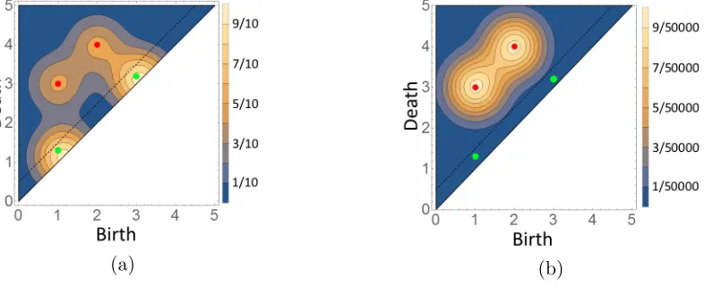
Example 1 Consider two 1-dimensional singleton diagrams, D1 and D2, with probabilities of being nonempty q(1) = 0.6 and q(2) = 0.8, respectively. The corresponding local densities when nonempty are given by p(1)(x) = √1
2πe
−(x+1)2/2
and p(2)(x) = √1 2πe
−(x−1)2/2
. Lemma 20 yields
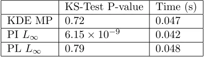
Figure 2: Left: Plot of the local density f1(x) in Eq. (3.13a). Right: Contour plot of the local density f2(x, y) in Eq. (3.13b). These pdfs cover the different possible input dimensions and are symmetric under permutations of the input.
f0 = P[|D| = 0] = (1−q(1))(1−q(2)) = 0.08, f1 = fD
R, and f2 = fD
R2. We sum over
permutations and divide by N! (N = 1,2 is the input cardinality) to obtain a symmetric global pdf.
f1(x) = (1−q(2))q(1)p(1)(x) + (1−q(1))q(2)p(2)(x) = √0.12
2πe
−(x+1)2/2
+ √0.32 2πe
−(x−1)2/2
, (3.13a)
f2(x, y) =
q(1)q(2)
2
h
p(1)(x)p(2)(y) +p(1)(y)p(2)(x)i = 0.24
2π
e−((x−1)2+(y+1)2)/2+e−((x+1)2+(y−1)2)/2
.
(3.13b)
Accounting for each cardinality and following Eq. (3.13a) and Eq. (3.13b), the total probability adds up to
P[|D|= 0] +P[|D|= 1] +P[|D|= 2] =f0+
Z
R
f1(x)dx+
Z
R2
f2(x, y)dxdy
= (0.08) + (0.12 + 0.32) + (0.24 + 0.24) = 1,
as desired. The local densities in Eq. (3.13a) and Eq. (3.13b) are plotted in Fig. 2. Though f1(x) is the sum of two Gaussians, in Fig. 2 (Left) we see that the Gaussian centered atx= 1 dominates, while the Gaussian centered at x=−1 is only indicated by a heavy left tail. This behavior occurs because q(2) = 0.8 is very close to 1.
4. Kernel Density Estimation
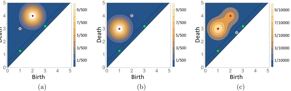
Generically, persistence diagrams have the majority of their points concentrated close to the diagonal. Consequently, the bandwidth σ is responsible for splitting a persistence diagram into upper and lower portions; see Eq. (4.1) and Fig. 3 (Left). The upper portion models the most topologically prominent points, which encompass topological information about the data, and its distribution reflects uncertainty in the precise location for prominent topological features in a persistence diagram. The lower portion models the majority of points in a persistence diagram. These points arise as a result of local noise in the underlying data, and in this fashion its distribution prescribes a noise likelihood model. Moreover, one can evaluate diagrams of any cardinality in the kernel (in this sense, the kernel is a global density). On the other hand, if one fixes the cardinality, one obtains the local kernel.
The construction of the kernel density proceeds by treating the upper and lower parts as inde-pendent, which necessitates the establishment of two density functions, one for each portion. The density for the upper part follows the recipe of Lemma 3.2 with a modified Gaussian chosen for
pj(ξ) in Eq. (3.9). To construct the kernel for the lower portion, we use (i) the number of points in D` to create a pertinent counting measure, and (ii) a modified Gaussian mixture with mean the projection of each point in D` to the diagonal. When evaluating a persistence diagram in the composite kernel, some of the points are evaluated in the density for the lower while others are evaluated in the density for the upper part. For a particular allocation of points to the upper and lower portions and by independence, the total evaluation follows from multiplying the results of these two evaluations together. However, since it is unknown a priori which input points should be used in each kernel, one must account for every possible partitioning of input points.
Section 4.1 gives a precise construction of of our kernel density estimator. In Section 4.2, we prove that our kernel density estimator converges to the true distribution as the number of persis-tence diagrams used to create it goes to infinity. Finally, Section 4.3 proposes a new statistic for persistence diagrams, the mean absolute bottleneck deviation (MAD), and establishes convergence of the sample MAD computed with our kernel density estimator.
4.1. Construction
We first define a random persistence diagram as a union of simpler constituents, and then determine its global pdf by combination in a fashion similar to Lemma 20. Indeed, we define the desired kernel density as the global pdf for this composite random diagram. To start, we fix a degree of homology
k and consider a center diagram D ⊂ Wk =W × {k} (see Eq. (2.1)). Since k is fixed, we treat
D ={ξi}Mi=1={(bi, di)}Mi=1 withinW =(b, d)∈R2 :d > b≥0 .
upper and lower portions according to a bandwidth σ as
Du ={(b
i, di, k)∈D :di−bi ≥σ} andD`={(bi, di, k)∈D:di−bi < σ}. (4.1)
Now define random diagramsDu centered atDuandD` centered atD`such thatD=Du∪D`. Ultimately, the global pdf ofD centered atD is our kernel density.
Definition 22 Each feature ξj = (bj, dj) ∈ Du yields an independent random singleton diagram Dj defined by its chance to be nonempty q(j) (via Eq. (4.3)) along with its potential position (b, d)
sampled according to a modified Gaussian distribution, denoted by N∗((bj, dj), σI). The global pdf for Du is then determined by Lemma 20, where each p(j) is given by the pdf associated with
N∗((bj, dj), σI), which is given by
p(j)(b, d) = R ϕj(b, d)
Wϕj(u, v)du dv
1W(b, d), (4.2)
where ϕj is the pdf of the (unmodified) normal N((bj, dj), σI), and 1W(·) is the indicator function
for the wedge.
The global pdf for each Dj is readily obtained by a pair of restrictions. First, we restrict the usual Gaussian distribution to the halfspace T =(b, d)∈R2:b < d . Features sampled below the diagonal are considered to disappear from the diagram and thus we define the chance to be nonempty by
q(j) =P(Dj 6=∅) =
Z
{v>u}
ϕj(u, v)du dv. (4.3)
Afterward, the Gaussian restricted to T is further restricted to W and renormalized to obtain a probability measure as in Eq. (4.2). This double restriction to both T and W is necessary for proper restriction of the Gaussian pdf and definition of q(j) = P(Dj 6= ∅). Indeed, restriction to W alone causes points with small birth time to have an artificially high chance to disappear; while restriction toT alone yields nonsensical features with negative radius (withb <0). In kernel density estimation, the effects of this distinction become negligible as the bandwidth goes to zero. In practice, this distinction is important for features with small birth time relative to the bandwidth.
Remark 23 In the ˇCech construction of a persistence diagram, a feature lies on the line b = 0
if and only if it has degree of homology k = 0. Consequently, for a feature (0, dj) with k = 0, we
instead take
p(j)(d) =R φj(d) R+φj(u)du
1R+(d) and q(j)=
Z
R+
φj(u)du
where φj is the 1-dimensional Gaussian centered at dj with standard deviation σ.
Definition 24 The lower random diagram D` is defined by choosing a cardinality N according to a pmf ν followed byN i.i.d. draws according to a fixed densityp`. First, take N`=
D`
and define
ν(·) with mean N` and so that ν(n) = 0 for n > mN` for some m > 0 independent of N`. The subsequent densityp`(b, d) is given by projecting the lower featuresD` of the center diagramD onto the diagonalb=d, then creating a restricted Gaussian kernel density estimation for these features; specifically,
p`(b, d) = 1
N`
X
(bi,di)∈D`
1
πσ2e −
b−bi+2di2+
d−bi+2di2
/2σ2
. (4.4)
Projecting the lower features D` of the center diagram D onto the diagonal simplifies later analysis and evaluation of p`; without projecting, a unique normalization factor, similar to q(j) in Def. 22, would be required for each Gaussian summand in Eq. (4.4). By Proposition 16 and Eq. (3.7), global pdfs of random persistence diagrams are described by a random vector pdf for each cardinality layer, resulting in the following global pdf forD`:
fD`(ξ1, ..., ξN) =ν(N)
N
Y
j=1
p`(ξj). (4.5)
Eq. (4.5) provides a noise model for the short-lived features near the diagonal. Combining the expressions forD` and Du, we arrive at the following proposition.
Proposition 25 Fix a center persistence diagram D and bandwidth σ >0. Split D into D` and
Du according to Eq. (4.1). Define D` with global pdf from Eq. (4.5), and Du with global pdf from
Eq. (3.9). Treating the random persistence diagramsDu andD` as independent, define their union
D. The following kernel density satisfies Def. 13 as the global pdf of D:
Kσ(Z,D) =
Nu
X
j=0
ν(N −j) X
γ∈I(j,Nu) Q(γ)
j
Y
k=1
p(γ(k))(ξk)
N
Y
k=j+1
p`(ξk), (4.6)
where Z = (ξ1, ..., ξN) is the input, ξi = (bi, di) for i = 1, ..., N are the features, and Nu = |Du|
depends on both D and σ. Here Q(γ) is given by Eq. (3.10), each p(j) refers to the modified
Gaussian pdf as shown in Eq. (4.2)for its matching featureξj in Du, andp` is given by Eq. (4.4).
Proof SinceDu and D`are independent random persistence diagrams, the belief function decom-poses intoβD(S) =βDu(S)βD`(S). Moreover, since derivatives above orderNu vanish forβDu (see
Remark 17), the product rule and binomial-type counting yield
δNβD δξ1...δξN
(∅) =
Nu
X
j=0
X
1≤i16=...6=ij≤N
δjβDu δξi1...δξij
(∅) δ
N−jβ D` δξ1...δξi1ˆ ...δξijˆ ...δξN
(∅)
= X
π∈ΠN Nu
X
j=0 1
j!(N −j)!
δjβDu δξπ(1)...δξπ(j)
(∅) δ
N−jβ D` δξπ(j+1)...δξπ(N)
(∅)
(4.7)
where δξˆi indicates that the given index is skipped in the set derivative (having been allocated to
permutation π ∈ ΠN; however, the ordering within each derivative is unrelated the choice of ij,
leading toj!-fold and (N −j)!-fold redundancy within each term. Taking Eq. (4.5) together with Eq. (3.7) yields
δβD` δξπ(j+1)...δξπ(N)
(∅) = (N −j)!ν(N −j)
N−j
Y
j=1
p`(ξj).
Also, Eq. (3.9) and Eq. (3.7) yield
δβDu
δξπ(1)...δξπ(j)(∅) =
X
π∗∈Π
j
X
γ∈I(j,Nu) Q(γ)
j
Y
k=1
p(γ(k))(ξπ∗(k)).
We substitute these relations into the final expression of Eq. (4.7). The first of these substitutions is straightforward, while the second has j!-fold redundant permutations overtop the existing per-mutations in ΠN. These substitutions yield that δ
NβD
δξ1...δξN(∅) =
P
π∈ΠNKσ(Z,D) as described in
Eq. (4.6) and shows that the kernel Kσ(Z,D) satisfies the definition of a global pdf for D (Def. 13). Finally, the sum over permutations is removed according to Eq. (3.7) to obtain the expression forfD(Z) =Kσ(Z,D).
Remark 26 A specific example of the component distributions provided for the kernel in Propo-sition 25 is presented in Fig. 3. Since the kernel density Kσ of Eq. (4.6) is a probability density
according to Def. 13, it is a function on ∪M
N=0W0:Nd−1, and so the sum of several such kernels is
defined by adding each local pdf layer separately.
Remark 27 In the definition of our kernel, a single parameter σ has been chosen for both the split of center diagrams, as well as the standard deviation used in the Gaussians which build our kernel. Without loss of generality, this choice simplifies the presentation of the kernel density and the proof of kernel density estimate (KDE) convergence (Theorem 31). In general, the bandwidth parameter σ2 which refers to the standard deviation used to define the Gaussians (as σ appears in
Defs. 22 and 24) need not be equal to the splitting parameter σ1 which determines which points
are in Du or D` (as σ appears in Eq. (4.1)). Still, it is certainly desirable that σ1 = Cσ2 when
taking a limit of KDEs as the number of persistence diagrams grows to infinity (Theorem 31). For a fixed kernel bandwidthσ2, increasingC (and thus σ1) moves more features into the lower portion
of the diagram. This choice may be useful in practice when underlying data are known to be noisy and more noise-related features are expected near the diagonal. By the same token, for σ1 >> σ2,
projecting the lower features onto the diagonal may lead to significant error in the approximation. On the other hand, taking σ1 << σ2 eliminates the computational benefit of splitting the diagram
and is probably not useful in practice. For most cases, taking σ1 = σ2, is a reasonable balance
between KDE accuracy and evaluation computation.
Since the kernel density is a probability density function for a random persistence diagram, it has an associated probability hypothesis density (See Def. 18).
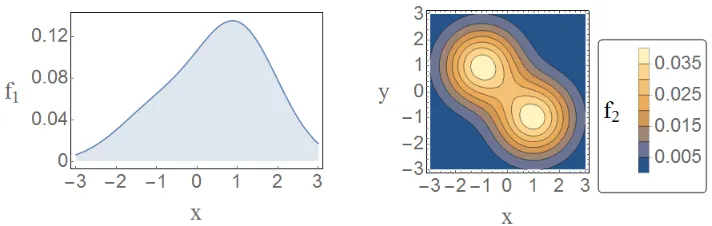
Figure 3: Left: A persistence diagram split according to Eq. (4.1). The dashed black line,d=b+σ, separates the diagram into the red upper points of Du and the yellow lower points of D`. Right:
The red and black gradients represent the upper singleton densitiesp(1)andp(2)given by Eq. (4.2). The green gradient represents the lower density p` defined in Eq 4.4. While each of these densities is defined on the wedge W ⊂ R2, the global kernel in Eq. (4.6) is defined on S
NWN for each
input-cardinality N.
Eq. (3.9). Treating the random persistence diagrams Du and D` as independent, the probability hypothesis density (PHD) associated with the kernel density centered at D with bandwidth σ of Theorem 25 is given by
Kσ,P HD(ξ,D) =N`p`(ξ) + Nu
X
j=1
q(j)p(j)(ξ), (4.8)
where the featureξ is the input and Nu =|Du|andN`=
D`
depend on both D and σ. Here each
p(j) refers to the modified Gaussian pdf as shown in Eq. (4.2)for its matching singleton feature ξj
in Du, q(j) given by (4.3) is the probability each singleton is present, and the lower density p` is
given by Eq. (4.4).
Proof The PHD is uniquely defined by its integral over a region U, which yields the expected number of points in the region. Consequently, the independent upper and lower random draws which build the kernel contribute additively to the PHD. Within the sum, each singleton density
p(j) is weighted by the chance for Dj to be present, q(j) and the lower density p` is weighted ac-cording to the mean draw cardinality, which was chosen to be D`
.
Remark 29 (Computational cost) The kernel density presented in Eq. (4.6) of Proposition 25 has approxmiately N!2Nu terms, necessitating shrewd computational strategies for real world usage. In practice, one may choose to consider only terms that correspond to high probability matchings. Such an implementation may be carried out with a linear assignment algorithm, like Munkres, resulting in a computational complexity of O(NuN3). Another approximation for the full kernel density is to consider input features as independent draws from the PHD given in (4.8) of Corollary 28. Evaluation of a diagram in Eq. (4.8) has time complexity O(N(Nu+N`)). Finally,
Notice that in Corollary 28, the input for the PHD is a single feature ξ as opposed to a list of features Z = {ξ1, ..., ξN} for the global kernel in Proposition 25. Furthermore, Proposition 25
extends to the analogue result for a center persistence diagram with features of varied degree of homology.
Corollary 30 Consider a persistence diagramD =Sd−1
k=0Dk× {k}split according to the degrees of
homology with associated random persistence diagrams Dk defined according to Eq. (4.6) for each
center diagram Dk. Treating each Dk as independent, the full global pdf for D=SDk centered at
D with bandwidth σ is given by
Kσ(Z,D) = Λ(N)
d−1
Y
k=0
Kσ(Zk,Dk), (4.9)
where Z = Sd−1
k=0Zk × {k} ⊂ W0:d−1 with each Zk ⊂ W of cardinality |Zk| = Nk within the
multi-index N = (N0, ..., Nd−1) and
Λ(N) = N! |N|! :=
Q
Nk!
(P
Nk)!.
Proof The result follows immediately from taking set derivatives of the full belief function
βD(S) = QkβDk(S). In particular, the set derivatives δβDk
δZ (∅) are zero unless Z ⊂ Wk. Thus,
the product rule leaves only the single term δβDδZ (∅) = Qd−1
k=0
δβDk
δZk (∅). In turn, each kernel global
pdfKσ(Zk,Dk) is related to the associated belief function derivative by a sum over permutations
ΠNk (see Eq. (3.7)). Compositions of these permutations are Nk!-fold redundant against the|N|!
permutations in Π|N|, yielding the coefficient Λ(N).
4.2. Convergence of the Kernel Density Estimator
In this section, to prove the convergence (to the target distribution) of the kernel density estimate defined via the kernel established in Proposition 25, we consider persistence diagrams{Di}ni=1which are i.i.d. sampled from a target distribution with global pdf f. Toward this end, we require the following assumptions on f:
(A1)f(Z) = 0 for |Z|> M ∈N (bounded cardinality).
(A2) The local densityfN :WkN →Ris bounded for eachN ∈ {1, ..., M}.
(A3) There existsCN >0 so thatf(ξ1, ..., ξN)≤CNk(ξ1, ..., ξN)k−2N for each N ∈ {1, ..., M}.
bounding death values by the diameter of the underlying dataset, one expects that the decay will be at worst a polynomial times Gaussian decay, which is sufficient for (A3).
The following theorem shows that the kernel density estimate converges to the true global pdf of a random persistence diagram as the number of persistence diagrams increases. The pdf tracks not only the birth and death of features, but also their prevalence. In particular, the persistence diagram pdf tied to a random dataset can determine which geometric features are stable regardless of their persistence.
Theorem 31 Consider a random persistence diagram global pdf f satisfying assumptions (A1)
-(A3). Define the kernelKσ(Z,D)according to Theorem 25 and consider the kernel density estimate
ˆ
f(Z) = n1Pn
i=1Kσ(Z,Di), with centers Di sampled i.i.d. according to global pdf f and bandwidth σ =O(n−α) chosen with 0< α < α2M. Then, asn→ ∞, fˆ→f uniformly on compact subsets of W.
Remark 32 The value of α2M is inherited from bandwidth selection for 2M-dimensional kernel
density estimates (Scott, 2015). While the scaling of the bandwidth in the limit is determined by the maximum cardinality M (and thus, the largest dimension of the local pdfs), choosing a bandwidth for a specific sample is an important step in applying kernel density estimation. If the bandwidth is too narrow, the estimate is overfitted and potentially biased; if the bandwidth is too large, the estimate will be oversmoothed, resulting in accuracy loss. Several methods for bandwidth selection in multivariate kernel estimation are discussed in (Silverman, 1986). As a general rule of thumb, (Silverman, 1986) recommends choosing the bandwidth as σopt=A(K)n−1/(d+4), where
n is the sample size (i.e., the number of persistence diagrams), d is the dimension, and A(K) is a constant depending on the kernel, K. In particular, one may choose α u 1/(2M + 4) as an
unbiased estimator for all local pdfs with cardinalities m ≤ M (Scott, 2015). Silverman’s rule of thumb works best for distributions which are nearly Gaussian; for more general distributions, the bandwidth may be chosen empirically.
Eq.(4.8) of Corollary 28 could be used as an approximation to the full kernel. The following argument verifies its convergence.
Corollary 33 Let Fg denote the P HD (Def. 18) of a random persistence diagram with global pdf g. Define fˆas in Thm 31. For a random persistence diagram whose global pdf f satisfies assumptions (A1)-(A3)of Thm 31, one hasFfˆ→Ff as n→ ∞ almost everywhere.
Proof LetC⊂W be compact. Define the counting function κC(Z) =|Z∩C|. Notice by Def. 18
that|R
CFfˆ(u)du−
R
CFf(u)du| ≤
R
WκC(Z)|fˆ(Z)−f(Z)|δZ ≤M(2M+1−1)
R
C|fˆ(Z)−f(Z)|δZ,
where the last inequality follows because we assume that random persistence diagrams are bounded byM andκC vanishes outside ofC. By Thm 31 and boundedness ofC, we can choosensufficiently
large to ensureRC|fˆ(Z)−f(Z)|δZ is arbitrarily small. Hence,RCFfˆ(u)du→
R
CFf(u)duasn→ ∞
on arbitrary compact subsets C. The result follows immediately by standard results in measure theory.
Throughout the proof we useξi to denote input features andZ ={ξ1, ..., ξN}orZ = (ξ1, ..., ξN)
to denote an input persistence diagram as a set or vector of features. Several preliminary lemmas are presented before the main body of the proof. We begin with a critical lemma which controls the number of features sampled in the band diagonal ∆βα={(b, d)∈W :α < d−b < β}.
Lemma 34 Consider a random persistence diagram D distributed according to f satisfying as-sumptions (A1)-(A3). Then there exists C >0 so thatEf(|∆σ0 ∩D|)≤Cσ.
Proof Consider a regionA⊂W and a counting functionκA(Z) =|Z∩A|such thatκA({ξ1, ..., ξN}) =
PN
i=11A(ξi). It is clear that this set function is well defined and measurable if A is measurable.
Using set integration (Def. 12),
E(|∆σ0 ∩D|) =
Z
W κ∆σ
0(Z)f(Z)δZ = M
X
N=0
N N!
Z
W
1∆σ 0(ξ1)
Z
f(ξ1, ...ξN)dξ2...dξN
dξ1 (4.10)
The expressions in Eq. (4.10) can be phrased in terms of the probability hypothesis density from Eq. (3.8), and for any choice ofL >0 are bounded by
Z
∆σ 0
FD(ξ)dξ≤
Z L
0
Z y
y−σ
FD(x, y)dx dy+
Z ∞
L
Z y
y−σ
C3y−2dx dy ≤LC2σ+ 3C3σ/L= (LC2+C3/L)σ
where assumptions (A2) and (A3) respectively yield the bounds C2 and C3y−2 on the probability hypothesis density,FD.
Lemma 34 yields control over the counting measure νi defined in Def. 24 and the coefficients Q∗i(·) of Eq. (3.11) which respectively determine the distribution of lower and upper cardinalities for a persistence diagram sampled according to the kernel densityKσ(Z,Di).
Corollary 35 Consider a random persistence diagramD distributed according to f satisfying as-sumptions (A1)-(A3). Take ν to be the lower cardinality probability mass function for the kernel density Kσ(Z, D) shown in Eq. (4.6). Then, there exists C >0 so that Efν(j0) ≤ Cσ whenever
j06= 0.
Proof Since D is random with respect tof,ν is random with respect tof as well. Recall thatν
is defined so thatEν(a) =D`
fora distributed according toν and thusEf[Eν(a)]≤Cσ for some
C >0 by Lemma 34. Subsequently, the value Efν(j0) is controlled by this double expectation so long as j0 6= 0. Indeed,
E(a) = ∞
X
j=0
jν(j) = ∞
X
j=1
jν(j)≥ ∞
X
j=1
ν(j)≥ν(j0)
for any j0>0 andνi(j0) = 0 for j0 <0 since it represents a cardinality distribution.
Lemma 36 Consider a random persistence diagram D distributed according to f satisfying as-sumptions (A1)-(A3). Take Q of Eq. (3.10) and Q∗ of Eq. (3.11) to be the upper singleton
probabilities for the kernel density Kσ(Z, D) shown in Eq. (4.6). Then, there exists C >0 so that
Ef[Q(γ)]≤Ef[Q∗(γ)]≤Cσ for any γ ∈I(j, N) with j < N.
Proof Since every q(k) ∈(0,1), we have that Q(γ) ≤ Q∗(γ); and furthermore, since γ ∈ I(j, N) are not onto when j < N, each product Q∗ is bounded by one of the terms of the (1−qi(k)) type. By construction, these terms depend monotonically upon a feature’s persistence, and the maximum (over all indices j < N and functionsγ) is tied to the least persistent feature of Diu.
For a feature (b, d) of persistence p = d−b, we define q(p) := R−∞p/(√ 2σ)
1 √
2πe
−x2/2
dx in
con-cordance with Eq. (4.3); or in terms of the error function Φ, q(p) = 12 1 + Φ 2pσ. Define the minimal persistence as pmin(Z) = sup{p:|∆p0∩Z|=∅} which satisfies pmin(Z) ≥p if and only if |∆p0∩Z|=∅. In turn, we may boundQ∗(γ)≤(1−q(p
min(D)) independently ofγ. By Lemma 34, there is C >0 such that Pf[|∆σ0 ∩D| 6=∅]≤Ef[|∆σ0 ∩D|]≤Cσ, which controls the distribution of the minimal persistence.
In particular, q0(p) = 2σ1√
πe
−p2/4σ2
by the fundamental theorem of calculus. The control of Lemma 34 and the fact that pmin(Z) ≥ 0 also allows us to use integration via the probability of sublevel sets. Take g(p) = 1−q(p) so that limp→∞g(p) = 0. Specifically, since Q∗(γ) ≤ (1−q(pmin(D)), and using the fundamental theorem of calculus then Fubini’s theorem, we have:
Ef[Q∗(γ)]≤
Z
W0:d−1
g(pmin(Z))f(Z)δZ=
Z
W0:d−1
Z pmin(Z)
∞
g0(p)dp
!
f(Z)δZ
=
Z 0
∞
Z
{Z:pmin(Z)<p}
f(Z)δZ
!
g0(p)dp=
Z ∞
0
Pf[pmin< p]
q0(p)dp.
(4.11)
We now further bound the expectation in Eq. (4.11). Replacing terms with their definitions and using the bound control from Lemma 34 we obtain:
Ef[Q∗(γ)]≤
Z ∞
0
Pf(∆p0∩D6=∅) 1 2σ√πe
−p2/4σ2 dp
≤ C 2σ√π
Z ∞
0
pe−(p/2σ)2dp= C 2σ√π
h
−2σ2e−p2/4σ2i
∞
p=0=
C
√
πσ.
Proof of Theorem 31. For convenience, we denote the upper cardinalities byNi =|Diu|and total
cardinalities byMi=|Di|for the sample persistence diagrams. Denote the set of strictly increasing
functions from {1, ..., j} into {1, ..., Ni} by I(j, Ni). Here we use ‘id’ to denote the identity map,
whereI(Ni, Ni) ={id}. The proof is organized by splitting the kernel densities into several pieces
First, we separate the kernel Kσ(Z,Di), defined in Eq. (4.6), into three portions, Ai,Bi, and Ci, according to the upper cardinalityj:
Kσ(Z,Di) = Ni
X
j=0
νi(N −j)
X
γ∈I(j,Ni) Qi(γ)
j
Y
k=1
p(iγ(k))(ξk) N
Y
k=j+1
p`i(ξk)
=νi(N−Ni)Qi(id) Ni
Y
k=1
p(ik)(ξk) N
Y
k=Ni+1
p`i(ξk)
+
Ni−1
X
j=0,j6=N
νi(N −j)
X
γ∈I(j,Ni) Qi(γ)
j
Y
k=1
p(iγ(k))(ξk) N
Y
k=j+1
p`i(ξk)
+1{n∈N:n<Ni}(N)νi(0) X
γ∈I(N,Ni) Qi(γ)
N
Y
k=1
p(iγ(k))(ξk)
=Ai+Bi+Ci,
(4.12)
where Ai follows fromj =Ni, Ci follows from j =N (Ci = 0 if Ni ≤N), and Bi consists of all remaining terms.
The terms Bi in Eq. (4.12) are controlled by the lower product
h QN
k=j+1p`i(ξk)
i
. Since (1−
qi(j))≤1 andνi(N −j)≤1 for any choice of γ and j, we have that Bi is bounded above by Ni−1
X
j=0,j6=N
X
γ∈I(j,Ni)
j
Y
k=1
qi(γ(k))pi(γ(k))(ξk) N
Y
k=j+1
p`i(ξk)
. (4.13)
The bounding sum of Eq. (4.13) consists of restricted 2N-dimensional Gaussians, with the weights
qi(j) dominating the restriction rescaling in Eq. (4.2). Fixπ ∈ ΠN and j ∈ {0, ..., M −1} \ {N}.
Without loss of generality, we treat the case when the permutation π is the identity. Since our ultimate goal is to control the kernel density estimate ˆf, consider the portion ofPn
i=1 1
nBi for which
the cardinalities Mi = |Di| are fixed at level Mi =m ∈ {0, ..., M}. Now, m =|Di| ≥ Ni > j, so
there is some extension for everyγ within the sum,γ∗∈Πm. Recall that this collection is random
because eachDiis randomly distributed according tof, therefore we consider the expectation with
respect to this randomness:
Ef
X
{i:Mi=m}
1 |{i:Mi =m}|
Mi
Y
k=1
q(γ
∗(k))
i p
(γ∗(k))
i (ξk)
→f(ξ1, ..., ξm),
for any point (ξ1, ..., ξm) as a 2m-dimensional Gaussian kernel density estimate with a proper choice
ofσ =O(n−α) appropriate for 2M (and hence 2m) dimensions (Scott, 2015). Integrating both sides against the extra coordinates, Assumptions (A2) and (A3) along with the dominated convergence theorem yield
Ef
X
{i:Mi=m}
1 |{i:Mi=m}|
j
Y
k=1
qi(γ(k))pi(γ(k))(ξk)
→ Z
Wm−j
which is again bounded via (A2) and (A3). Of course,|{i:Mi =m}| ≤n, so taking Eq. (4.14) into account for everymbounds the averaging sum of the upper product: 1nPn
i=1
Qj
k=1q (γ(k))
i p
(γ(k))
i (ξk).
Relying on Eq. (4.13), we must also consider the lower productQN
k=j+1p`i(ξk). Since the points ξi are fixed, we focus on their minimal persistencepmin = mini(di−bi). Thus,
p`i(ξi)≤ 1 2πσ2e
−(b−d)2/4σ2
≤ 1 2πσ2e
−p2 min/4σ2,
and subsequently,
N
Y
k=j+1
p`i(ξk)
≤
1 (2πσ2)Ne
−N p2
min/4σ2 →0, (4.15)
asσ →0, uniformly on any compact subset ofW (or W0:d−1). Altogether, Eqs. (4.14) and (4.15) guarantee that the term Pn
i=1 n1Bi→0 as n→ ∞ in the kernel density estimation.
Next we focus on the terms Ai in Eq. (4.12). We split the sum 1nPn
i=1Ai according to the cardinality of Di. Specifically, separate Ai into the cases where Mi =6 Ni or Mi = Ni. First
consider the associated set of indices {i:Mi6=Ni} and define the mismatch number MM(n) to
be its cardinality. Critical to our argument, the mismatch number is random with respect to f
because it is defined according to the features inDi. We obtain the following mismatched term:
1
n
X
{i:Ni6=Mi}
Ai≤
M M(n)
n
1
M M(n)
X
{i:Ni6=Mi}
Qi(id) Ni
Y
k=1
p(ik)(ξk) N
Y
k=Ni+1
p`i(ξk)
(4.16)
The bounding sum in Eq. (4.16) is split into pieces where Mi =m for eachm between 0 and M. Using the same strategy yielding Eq. (4.14), with M M(n) in place of n, the sum of the upper product converges to layered integrals off for each level mand each Ni< mby extending γ = id.
Using the same approach leading to Eq. (4.15), the lower product vanishes in the limit ifNi6=N, or is an empty product ifNi=N; in either case, this factor is bounded. Now, according to Lemma
34, Pf(Mi 6=Ni) =Pf(Di∩∆σ0 6=∅) ≤C5σ; consequently, Ef[M M(n)/n]→0 and the mismatch terms on left hand side of Eq. (4.16) follow.
Now consider the indices for which Ni = Mi. In this case, since Di` are empty, νi = δ0, and the only values which contribute to the sum are for Ni =N. The remaining portion of the kernel
density estimate is given by
1
nE
f X
{i:Ni=Mi}
Ai =
1 nE f X
{i:Ni=Mi}
Qi(id)
N
Y
k=1
p(ik)(ξk)
! = 1 nE f X
{i:Ni=Mi}
N
Y
k=1
q(ik)p(ik)(ξk)
!
.
(4.17)
As shown, the terms in Eq. (4.17) are restricted 2N dimensional Gaussians. It is known (Scott,
2015) that restricted Gaussian kernel density estimates like
h QN
k=1q (k)
i p
(k)
i (ξk)
i
converge (uniformly on compactly contained sets) to the true value of the chosen draws Di for a suitable choice of α
in σ = O(n−α) as restricted by N ≤ M. After correcting for the samples with Ni < Mi = N,
that the target distribution associated with hQN
k=1q (k)
i p
(k)
i (ξk)
i
is the rescaled f(1N)f(ξ1, ..., ξN),
wheref(N) :=Pf(|D|=N). This rescaling for the conditional pdff(D| |D|=N) is necessary to reweight according to Proposition 16.
Application of classical kernel density estimate results require division by the cardinality of the draw, when in context n is generally larger than this cardinality. Thus, we must again consider the cases whereinNi 6=Mi. Consequently, we find that the expectation for the ratio between the true draw cardinality and nis given by Pf(|D|=N) +O(σ) according to Lemma 34. Indeed, this ratio converges tof(N) :=Pf(|D|=N). After this final correction, we have shown that n1Pni=1Ai
approach the true pdff(ξ1, ..., ξN).
Lastly, we need only to control the terms Ci from Eq. (4.12). We begin by bounding the probability mass functionsνi by 1 and considering only terms for which the characteristic function
is nonzero: 1 n n X i=1
Ci =
1
n
X
{i:N <N}
νi(0)
X
γ∈I(N,Ni) Qi(γ)
N
Y
k=1
p(iγ(k))(ξk)≤
1
n
X
{i:N <Ni}
X
γ∈I(N,Ni) Qi(γ)
N
Y
k=1
p(iγ(k))(ξk).
(4.18) Next, we split the term Q(γ) according to Eq. (3.10) and apply Lemma 36 to the upper bound in Eq. (4.18) to obtain the larger upper bound
1
n
X
{i:N <Ni}
X
γ∈I(N,Ni) Q∗(γ)
N
Y
k=1
qi(γ(k))pi(γ(k))(ξk)≤C
1
n
X
{i:N <Ni}
X
γ∈I(N,Ni)
N
Y
k=1
qi(γ(k))pi(γ(k))(ξk)
σ.
(4.19)
The expectation of the bracketed terms in Eq. (4.19) converges in a fashion identical to the terms 1nPn
i=1Ai. Since these terms are multiplied by σ, altogether
1
n
Pn i=1Ci
vanishes in the limit asn→ ∞. Putting together the limits of each portion built fromKσ(Z,Di) =Ai+Bi+Ci,
the theorem follows.
4.3. A Measure of Dispersion
Theorem 31 has established the convergence of a kernel density estimator. Along with density function estimation, one would like to verify the convergence of properties such as spread. In the absence of vector space structure on the space of persistence diagrams, we turn to the bottleneck metric (Def. 5) to define a notion of spread. Specifically, we measure dispersion with respect to a distribution of persistence diagrams through its mean absolute deviation in this metric.
Definition 37 The mean absolute bottleneck deviation (MAD) from origin diagramD with respect to a global pdf f is given by
MADf(D) =
Z
W0:d−1
W∞(D, Z)f(Z)δZ (4.20)
Proposition 38 ConsiderD distributed according to the kernel density Kσ(·,D) with center dia-gram D and bandwidth σ. Fix δ ≥1. Then,
P[W∞(D,D)< δσ]≥
Z
B(0,δ) 1 2πe
−(x2+y2)/2 dx dy
!M
(4.21)
where M is the maximal cardinality of D (a multiple of |D|). Here B(x, r) refers to a ball with respect to the infinity metric (as is used in bottleneck distance).
Next, we relax assumption (A2) by considering the entire multi-wedge W0:d−1 and tighten the decay control from assumption (A3). Formally,
(A2)∗ The local density fN :W0:Nd−1 →Ris bounded for eachN ∈ {1, ..., M}.
(A3)∗ There exists C >0 so that f(ξ1, ..., ξN)≤Ck(ξ1, ..., ξN)k−2N−2 forN ∈ {1, ..., M}.
These assumptions (and (A1)) are required for the subsequent lemma, which ensures that the mean absolute bottleneck deviation (MAD) is finite.
Lemma 39 Consider a random persistence diagramD distributed according to a global pdf f sat-isfying assumptions (A1), (A2)∗, and (A3)∗. Then D has finite MAD for any choice of origin diagram D.
Similar to assumption (A3) (given prior to Theorem 31), (A3)∗ holds for a random persistence diagram associated with underlying data sampled from a compact set perturbed by Gaussian noise. One may also replace Lemma 39 and its assumptions by directly assuming that the maximal persistence moment is bounded; with this, the results of Lemma 39 follow immediately from Eq. (A.3) in the supplementary. This direct assumption is weaker (implied by (A1), (A2)∗, and (A3)∗), but may be difficult to show directly in practice.
Theorem 40 Consider a distribution of persistence diagrams with bounded global pdf,f, satisfying assumptions (A1), (A2)∗, and (A3)∗. Let fˆ(Z) = 1nPn
i=1Kσ(Z,Di) be a kernel density estimate
with centers Di sampled i.i.d. according to global pdf f and bandwidth σ = O(n−α) chosen with
0< α < α2M. Then, the mean absolute bottleneck deviation estimate converges; in other words,
Z
W0:d−1
W∞(D0, Z) ˆf(Z)δZ →
Z
W0:d−1
W∞(D0, Z)f(Z)δZ (4.22)
as n→ ∞ for any origin diagram D0.
Proof The MAD off with originD0is finite by Lemma 39. To show convergence of the estimate, we begin by adding and subtracting the integral of the sample estimator for the MAD. Then, we split the sum inton+ 1 terms via the triangle inequality to obtain
Z
W0:d−1
W∞(D0, Z)f(Z)δZ−
Z
W0:d−1
W∞(D0, Z) ˆf(Z)δZ
≤ Z
W0:d−1
W∞(D0, Z)f(Z)δZ− 1 n n X i=1 Z
W0:d−1
W∞(D0,Di)Kσ(Z,Di)δZ
+1 n n X i=1 Z
W0:d−1
W∞(D0, Z)Kσ(Z,Di)δZ−
Z
W0:d−1
W∞(D0,Di)Kσ(Z,Di)δZ

![Figure 4: Cardinality probabilities P[|D| = N] for random diagram D distributed according toglobal pdf Kσ(·, D) in Ex](https://thumb-us.123doks.com/thumbv2/123dok_us/9775975.1962847/28.612.245.365.94.171/figure-cardinality-probabilities-random-diagram-distributed-according-toglobal.webp)