The
xyz
algorithm for fast interaction search in
high-dimensional data
Gian-Andrea Thanei [email protected]
Seminar f¨ur Statistik ETH Z¨urich
8092 Z¨urich, Switzerland
Nicolai Meinshausen [email protected]
Seminar f¨ur Statistik ETH Z¨urich
8092 Z¨urich, Switzerland
Rajen D. Shah∗ [email protected]
Statistical Laboratory University of Cambridge Cambridge, CB3 0WB, UK
Editor:Jennifer Dy
Abstract
When performing regression on a data set with p variables, it is often of interest to go beyond using main linear effects and include interactions as products between individual variables. For small-scale problems, these interactions can be computed explicitly but this leads to a computational complexity of at least O(p2) if done naively. This cost can be prohibitive ifpis very large.
We introduce a new randomised algorithm that is able to discover interactions with high probability and under mild conditions has a runtime that is subquadratic in p. We show that strong interactions can be discovered in almost linear time, whilst finding weaker interactions requires O(pα) operations for 1 < α < 2 depending on their strength. The underlying idea is to transform interaction search into a closest pair problem which can be solved efficiently in subquadratic time. The algorithm is calledxyz and is implemented in the languageR. We demonstrate its efficiency for application to genome-wide association studies, where more than 1011 interactions can be screened in under 280 seconds with a
single-core 1.2 GHz CPU.
Keywords: interactions, high-dimensional data, regression, computational tradeoffs, close pairs
1. Introduction
Given a response vector Y ∈Rn and matrix of associated predictors X = (X1, . . . ,Xp) ∈
Rn×p, finding interactions is often of great interest as they may reveal important
relation-ships and improve predictive power. When the number of variablespis large, fitting a model involving interactions can involve serious computational challenges. The simplest form of
∗. Supported by the Isaac Newton Trust Early Career Support Scheme, the Alan Turing Institute under the EPSRC grant EP/N510129/1 and EPSRC Programme Grant EP/N031938/1
c
interaction search consists of screening for pairs (j, k) with high inner product between the outcome of interest Y and the point-wise product Xj◦Xk:
Keep all pairs (j, k) for whichYT(Xj ◦Xk)/n > κ. (1)
This search is of complexity O(np2) in a naive implementation and quickly becomes infea-sible for largep. Of course one would typically be interested in maximising (absolute values of) correlations rather than dot products in (1), an optimisation problem that would be at least as computationally intensive.
Even more challenging is the task of fitting a linear regression model involving pairwise interactions:
Yi =µ+
p X
j=1
Xijβj+
p X
k=1
k−1
X
j=1
XijXikθjk+εi. (2)
Hereµ∈Ris the intercept andβj and θjk contain coefficients for main effects and
interac-tions respectively, andεi is random noise.
In this paper, we make several contributions to the problem of searching for interactions in high-dimensional settings.
(a) We first establish a form of equivalence between (1) and closest-pair problems (Shamos and Hoey, 1975; Agarwal et al., 1991). Assume for now that all predictors and outcomes are binary, so Xij, Yi ∈ {−1,1} (we will later relax this assumption) and define Z ∈
{−1,1}n×p asZ
ij =YiXij. Then it is straightforward to show that (1) is equivalent to
Keep all pairs (j, k) for which kXj −Zkk2 < κ0 (3) for some κ0. This connects the search for interactions to literature in computational geometry on problems of finding closest pairs of points.
(b) We introduce the xyz algorithm to solve (3) based on randomly projecting each of the columns in X and Z to a one-dimensional space. By exploiting the ability to sort the resulting 2p points with O(plog(p)) computational cost, we achieve a run time that is always subquadratic inpand can even reach a linear complexityO(np) whenκis much larger than the quantity|YT(Xj◦Xk)|/nof the bulk of the pairs (j, k). We show that
our approach can be viewed as an example of locality sensitive hashing (Leskovec et al., 2014) optimised for our specific problem.
(c) We show how any method for solving (1) can be used to fit regression models with interactions (15) by building it into an algorithm for the Lasso (Tibshirani, 1996). The use of xyz thus leads to a procedure for applying the Lasso to all main effects and interactions with computational cost that scales subquadratically inp.
1.1 Related work
A common approach to avoid the quadratic cost in p of searching over all pairs of vari-ables (1) is to restrict the search space: one can first seek a small number of important main effects, and then only consider interactions involving these discovered main effects. More specifically, one could fit a main effects Lasso (Tibshirani, 1996) to the data first, add interactions between selected main effects to the matrix of predictors, and then run the Lasso once more on the augmented design matrix in order to produce the final model (see Wu et al. (2010) for example). Tree-based methods such as CART (Breiman et al., 1984) work in a similar fashion by aiming to identify an important main effect and then only considering interactions involving this discovered effect.
However it is quite possible for the signal to be such that main effects corresponding to important interactions are hard to detect. As a concrete example of this phenomenon, consider the setting whereXis generated randomly with all entries independent and having the uniform distribution on{−1,1}. Suppose the response is given byYi =Xi1Xi2, so there
is no noise. Since the distributionYi|Xij is the same for allk, main effects regressions would
find it challenging to select variables 1 and 2. Note that by reparametrising the model by adding one to each entry ofX for example, we obtainYi = (Xi1−1)(Xi2−1) = 1−Xi1−
Xi2 +Xi1Xi2. The model now respects the so-called strong hierarchical principle (Bien et al., 2013) that interactions are only present when their main effects are. The hierarchical principle is useful to impose on any fitted model. However, imposing the principle on the model does not imply that the interactions will easily be found by searching for main effects first. The difficulty of the example problem is due to interaction effects masking main effects: this is a property of the signalE(Yi) and of course no reparametrisation can
make the main effects any easier to find. Approaches that increase the set of interactions to be considered iteratively can help to tackle this sort of issue in practice (Bickel et al., 2010; Hao and Zhang, 2014; Friedman, 1991; Shah, 2016) as can those that randomise the search procedure (Breiman, 2001). However they cannot eliminate the problem of missing interactions, nor do these approaches offer guarantees of how likely it is that they discover an interaction.
As alluded to earlier, the pure interaction search problem (3) is related to close pairs of points problems, and more specifically the close bichromatic pairs problem in computa-tional geometry (Agarwal et al., 1991). Most research in this area has focused on algorithms that lead to computationally optimal results in the number of points p whilst considering the dimension n to be constant. This has resulted in algorithms where the scaling of the computational complexity with n is at least of order 2n (Shamos and Hoey, 1975). Since for meaningful statistical results one would typically require nlog(p), these approaches would not lead to subquadratic complexity. An exception is the so-called lightbulb algo-rithm (Paturi et al., 1989) which employs a similar strategy for binary data; our work here shows that this is optimal among random projection-based methods and also that it may be modified to handle continuous data and also detect interactions in high-dimensional regression settings.
In the special case wheren=pandZij, Xij ∈ {−1,1}, (3) may be seen to be equivalent
deliver a subquadratic complexity of roughly O(p2.4) = O(np1.4) (Williams, 2012; Davie and Stothers, 2013; Le Gall, 2012). However the constants hidden in the order notation are typically very large, and practical implementations are unavailable. The Strassen algorithm (Strassen, 1969) is the only fast matrix multiplication algorithm used regularly in practice to the best of our knowledge. With a complexity of roughly O(p2.8) = O(np1.8), the improvement over a brute force close pairs search is only slight.
The strategy we use is most closely related to locality sensitive hashing (LSH) (Indyk and Motwani, 1998) which encompasses a family of hashing procedures such that similar points are mapped to the same bucket with high probability. A close pair search can then be conducted by searching among pairs mapped to the same bucket. In fact, our approach for solving (3) can be thought of as an example of LSH optimised for our particular problem setting. This connection is detailed in Appendix B.
A seemingly attractive alternative to the subsampling-based LSH-strategy we employ is the method of random projections which is motivated by the theoretical guarantees offered by the Johnson–Lindenstrauss Lemma (Achlioptas, 2003). Perhaps surprisingly, we can show that using random projections instead of our subsampling-based scheme leads to a quadratic run time for interaction search (see Theorem 1 and section 5.1).
An approach that bears some similarity with our procedure is that ofepiq (Arkin et al., 2014). This works by projecting the data and then searches through a lower dimensional representation for close pairs. This appears to improve upon a naive brute force empirically but there are no proven guarantees that the run time improves on the O(np2) complexity of a naive search.
TheRandom Intersection Trees algorithm of Shah and Meinshausen (2014) searches for potentially deeper interactions in data with both X and Y binary. In certain cases with strong interactions a complexity close to linear inp is achieved; however it is not clear how to generalise the approach to continuous data or embed it within a regression procedure.
The idea of Kong et al. (2016) is to first transform the data by forming ˜Y = Y◦Y
and ˜Xj = Xj ◦Xj for each predictor. Next ˜Xj and ˜Y are tested for independence using the distance correlation test. In certain settings, this can reveal important interactions with a computational cost linear in p. However, the powers of these tests depend on the distributions of the transformed variables ˜Xj. For example in the binary case when X ∈ {−1,1}n×p, each transformed variable will be a vector of 1’s and the independence tests
will be unhelpful. We will see that our proposed approach works particularly well in this setting.
1.2 Organisation of the paper
demonstrate how the xyz algorithm can be embedded within common algorithms for high-dimensional regression (Friedman et al., 2010) allowing high-high-dimensional regression models with interactions to be fitted with subquadratic complexity inp. Section 5 contains a variety of numerical experiments on real and simulated data that complement our theoretical results and demonstrate the effectiveness of our proposal in practice. We conclude with a brief discussion in Section 6 and all proofs are collected in the Appendix.
2. The xyz algorithm for binary data
In this section, we present a version of thexyz algorithm applicable in the special case where bothXandY are binary, soXij ∈ {−1,1}andYi∈ {−1,1}. We build up to the algorithm
in stages, giving the final version in Section 2.2. Define Z∈ {−1,1}n×p by Z
ij =YiXij and
γjk =
1
n n X
i=1
1{Yi=XijXik}. (4)
We callγjk the interaction strength of the pair (j, k). It is easy to see that the interaction
search problem (1) can be expressed in terms of either the γjk or the normalised squared
distances. Indeed
2γjk−1 =YT(Xj◦Xk)/n=ZTjXk/n= 1− kZj−Xkk22/(2n). (5) Thus those pairs (j, k) with YT(Xj ◦Xk)/n large will have γjk large, and kZj −Xkk22 small. This equivalence suggests that to solve (1), we can search for pairs (j, k) of columns
Zj,Xk that are close in `2 distance. At first sight, this new problem would also appear to involve a search across all pairs, and would thus incur an O(np2) cost. As mentioned in the introduction, close pair searches that avoid a quadratic cost in p incur typically an exponential cost in n. Since n would typically be much larger than log(p), such searches would be computationally infeasible.
We can however project each of then-dimensional columns ofXandZto a lower dimen-sional space and then perform a close pairs search. The Johnson–Lindenstrauss Lemma, which states roughly that one can project p points into a space of dimension O(log(p)) and faithfully preserve distances, may appear particularly relevant here. The issue is that the projected dimension suggested by the Johnson–Lindenstrauss Lemma is still too large to allow for an efficient close pairs search. The following observation however gives some encouragement: if we had Y = Xj ◦Xk so Xj = Zk, even a one-dimensional projection R∈Rnwill have|RT(X
j−Zk)|= 0 =kXj−Zkk2, which implies that a perfect interaction will have zero distance in the projected space. We will later see that our approach leads to a linear run time in such a case. Importantly, we are only interested in using a projection that preserves the distances between the close pairs rather than all pairs, which makes our problem very different to the setting considered in the Johnson–Lindenstrauss Lemma.
With this in mind, consider the following general strategy. First project the columns of X and Zto one-dimensional vectors x and z using a random projection R: x=XTR,
z = ZTR. Next for some threshold τ, collect all pairs (j, k) such that |xj −zk| ≤ τ in
for example Sedgewick (1998)), this close pairs search can be shown to be very efficient. Given this set of candidate interactions, we can check for each (j, k)∈E whether we have
γjk ≥γ. The process can be repeated L times with different random projections, and one
would hope that given enough repetitions, any given strong interaction would be present in one of the candidate sets E1, . . . , EL with high probability. This approach is summarised
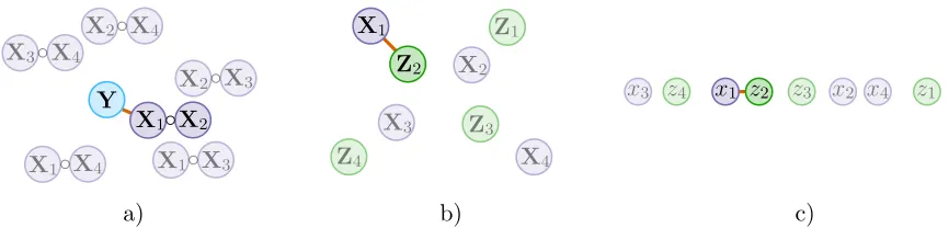
in Algorithm 1 which we term the general form of thexyz algorithm. A schematic overview is given in Figure 1.
Algorithm 1 A general form of thexyz algorithm.
Input: X∈ {−1,1}n×p,Y∈ {−1,1}n
Parameters: ξ= (G, L, τ, γ). HereGis the joint distribution for the projection vector
R, L is the number of projections, and τ and γ are the thresholds for close pairs and interactions strength respectively.
Output: I set of strong interactions.
1: FormZvia Zij =YiXij and setI :=∅.
2: forl∈ {1, . . . , L} do
3: Draw random vector R∈Rn with distribution Gand project the data using R, to
form
x=XTR andz=ZTR. 4: Collect in El all pairs (j, k) such that |xj−zk| ≤τ. 5: Add to I those (j, k)∈El for which γjk ≥γ. 6: end for
There are several parameters that must be selected, and a key choice to be made is the form of the random projectionR. For the joint distributionGofRwe consider the following general class of distributions, which includes both dense and sparse projections. We sample a random or deterministic number M of indices from the set {1, . . . , n},i1, . . . , iM, either
with or without replacement. Then, given a distribution F ∈ F where F is a class of distributions to be specified later, we form a vectorD∈RM with independent components
each distributed according toF. We then define the random projection vector Rby
Ri =
M X
m=1
Dm1{im=i}, i= 1, . . . , n. (6)
Each configuration of the xyz algorithm is characterised by fixing the following param-eters:
(i) G, a distribution for the projection vectorRwhich is determined through (6) byF ∈ F, a distribution for the subsample sizeM and whether sampling is with replacement or not;
(ii) L∈N, the number of projection steps; (iii) τ ≥0, the close pairs threshold;
We will denote the collection of all possible parameter levels by Ξ. This includes the following subclasses of interest. FixF ∈ F.
(a) Dense projections. LetR∈Rnhave independent components distributed according
to F and denote the distribution of R by G. This falls within our general framework above with M set ton and sampling without replacement. Let
Ξdense :={ξ∈Ξ with joint distribution equal to G}.
(b) Subsampling. Let Gsubsample be the set of distributions for R obtained through (6) when subsampling with replacement. Let
Ξsubsample :={ξ∈Ξ : joint distributionG∈ Gsubsample}.
(c) Minimal subsampling. Let Ξminimal be the set of all parameters in Ξsubsample such that the close pairs threshold isτ = 0 andM takes randomly values in the set{m, m+1}
for some positive integer m.
Ξminimal:={ξ∈Ξsubsample with τ = 0 and M ∈ {m, m+ 1} for somem∈N}.
Note that we have suppressed the dependence of the classes above on the fixed distribution
F ∈ F for notational simplicity. We define F to be the set of all univariate absolutely continuous and symmetric distributions with bounded density and finite third moment. The restriction to continuous distributions in F ensures that Ξminimal is invariant to the choice of F: whenτ ≡0, every F ∈ F with L∈Nand the distribution forM fixed yields the same algorithm. Moreover the set of close pairs in Cl is simply the set of pairs (j, k)
that have Ximj =Zimk for allm = 1, . . . , M, that is the set of pairs that are equal on the subsampled rows. We note that the symmetry and boundedness of the densities inF and finiteness of the third moment are mainly technical conditions necessary for the theoretical developments in the following section. We will assume without loss of generality that the second moment is equal to 1. This condition places no additional restriction on Ξ since a different second moment may be absorbed into the choice of τ.
Minimal subsampling represents a very small subset of the much larger class of ran-domised algorithms outlined above. However, Theorem 1 below shows that minimal sub-sampling is essentially always at least as good as any algorithm from the wider class, which is perhaps surprising. A beneficial consequence of this result is that we only need to search for the optimal ways of selecting M and L; the threshold τ is fixed atτ = 0 and the choice of the continuous distribution F is inconsequential for minimal subsampling. The choices we give in Section 2.2 yield a subquadratic run time that approaches linear in p when the interactions to be discovered are much stronger than the bulk of the remaining interactions.
2.1 Optimality of minimal subsampling
a) b) c)
Figure 1: Illustration of the general xyz algorithm. The strongest interaction is the pair (1,2) andp= 4. Panel a) illustrates the interaction search among Yand Xj◦Xk, panel b) shows the closest pair problem after the transformation Zij = XijYi and panel c) depicts
the closest pair problem after the data has been projected. These are the three main steps in thexyz algorithm.
a strongest interaction pair, that is γj∗k∗ = maxj,k∈{1,...,p}γjk. We will consider algorithms
ξ with γ set to γj∗k∗. Define the power ofξ∈Ξ as
Power(ξ) :=Pξ((j∗, k∗)∈I).
Forη ∈(0,1), let
Ξdense(η) ={ξ ∈Ξdense : Power(ξ)≥η},
and define Ξsubsample(η) and Ξminimal(η) analogously. Note that these classes depend on the underlyingF ∈ F, which is considered to be fixed, and moreover that we are fixingγ =γj∗k∗. We consider an asymptotic regime where we have a sequence of response–predictor matrix pairs (Y(n),X(n))∈
Rn×Rn×pn. Writeγjk(n)for the corresponding interaction strengths, and
letγ1(n) = maxj,kγjk(n). Letfγ(n) be the probability mass function corresponding to drawing
an element of γ(n) uniformly at random. Note that fγ(n) has domain{0,1/n,2/n, . . . ,1}.
We make the following assumptions about the sequence of interaction strength matrices
γ(n).
(A1) There existsc0 such that|{(j, k) :γjk(n)=γ(1n)}| ≤c0pn.
(A2) There existsγl>0, γu <1 such thatγu ≥γ1(n) ≥γl for all n.
(A3) There existsρ <1 such thatfγ(n) is non-increasing on [ργ
(n) 1 , γ
(n)
1 )∩ {0,1/n, . . . ,1}.
Assumption (A1) is rather weak: typically one would expect the maximal strength interac-tion to be essentially unique, while (A1) requires that at most of orderpninteractions have
maximal strength. (A2) requires the maximal interaction strength to be bounded away from 0 and 1, which is the region where complexity results for the search of interactions are of interest. As mentioned earlier, if the maximal interaction strength is 1, it will always be retained in the close-pair sets Cl, whilst if its strength is too close to 0, then it is near
To aid readability, in the following we suppress the dependence of quantities onnin the notation. Given X and Y, we may define T(ξ) as the expected number of computational operations performed by the algorithm corresponding to ξ. We have the following result.
Theorem 1 Given F ∈ F and η∈(0,1), there exists n0 such that for all n≥n0 we have inf
ξ∈Ξminimal(η)T(ξ) = ξ∈Ξsubsample(inf η)T(ξ), (7) inf
ξ∈Ξminimal(η)
T(ξ)
np2 → 0, (8)
and there existsc >0 such that
inf
ξ∈Ξdense(η)
T(ξ)
np2 > c. (9)
The theorem shows that the optimal run time is achieved when using minimal subsam-pling. The last point is surprising: setting R∼ N(0,I), for example, will not improve the computational complexity over the brute-force approach and dense Gaussian projections hence do not reduce the complexity of the search. This is not caused by the larger com-putational effort involved in computing the dense projections: indeed even if these could be computed for free this result would remain. Rather the cost stems from the fact that dense projections have a much lower power for detecting true close pairs in the projected one-dimensional space.
2.2 The final version of xyz
The optimality properties of minimal subsampling presented in the previous section suggest the approach set out in Algorithm 2, which we will refer to as thexyz algorithm. Here we
Algorithm 2 Final version of the xyz algorithm.
Input: X ∈ {−1,1}n×p, Y ∈ {−1,1}n, subsample size M, number of projections L,
threshold for interaction strengthγ.
Output: I set of strong interactions.
1: FormZvia Zij =YiXij.
2: forl∈ {1, . . . , L} do
3: FormR∈Rn as in (6) with distributionF =U[0,1] and setx=XTR,z=ZTR.
4: Find all pairs (j, k) such thatxj =zk and store these inEl. 5: Add to I those pairs inEl for which γjk ≥γ.
6: end for
4
6
7
2
3
5
1
9
8
3
2
4
1
5
7
6
9
8
Figure 2: Illustration of an equal pairs search among components ofx,z∈Rp whenp= 9.
The horizontal locations of blue and green circles numbered j give xj and zj respectively.
Sorting of (x,z) allows traversal of the unique locations. At each of these it is checked whether points of both colours are present, and if so, the indices are recorded. Here the set of equal pairs ({3} × {4,6})∪({5} × {2})∪({7,9} × {1,5}) would be returned.
To perform the equal pairs search in line 4, we sort the concatenation (x,z) ∈ R2p to
determine the unique elements of {x1, . . . , xp, z1, . . . , zp}. At each of these locations, we
can check if there are components from both x and z lying there, and if so record their indices. This procedure, which is illustrated in Figure 2, gives us the set of equal pairs E
in the form of a union of Cartesian products. The computational cost is O(plog(p)). This complexity is driven by the cost of sorting whilst the recording of indices is linear inp. We note, however, that looping through the set of equal pairs in order to output a list of close pairs of the form (j1, k1), . . . ,(j|E|, k|E|) would incur an additional cost of the size of E, though in typical usage we would have |E|=o(p). Readers familiar with locality sensitive hashing (LSH) can find a short interpretation of equal pairs search as an LSH-family in the appendix. In the next section, we discuss in detail the impact of minimal subsampling on the complexity of thexyz algorithm and the discovery probability it attains.
2.3 Computational and statistical properties of xyz
We have the following upper bound on the expected number of computational operations performed byxyz (Algorithm 2) when the subsample size and number of repetitions areM
and L:
C(M, L) :=np
(i)
+L{M p
(ii)
+plog(p) (iii)
+nEξ(|E1|) (iv)
}. (10)
The terms may be explained as follows: (i) construction ofZ; (ii) multiplyingM subsampled rows of X and Z by R ∈ Rn; (iii) finding the equal pairs; (iv) checking whether the
interactions exceed the interaction strength threshold γ. Note we have omitted a constant factor from the upper bound C(M, L). There is a lower bound only differing from (10) in the equal pairs search term (iii), which is p instead of plog(p). It will be shown that (iv) is the dominating term and therefore the upper and lower bound are asymptotically equivalent, implying the bounds are tight.
An interaction with strengthγ is retained inE1 with probabilityγM. Hence it is present in the final set of interactions I with probability
The following result demonstrates how the xyz algorithm can be used to find interactions whilst incurring only a subquadratic computational cost.
Theorem 2 Let FΓ be the distribution function corresponding to a random draw from the set of interaction strengths {γjk}j,k∈{1,...,p}. Given an interaction strength threshold γ, let 1−FΓ(γ) =c1/p. Defineγ0 =p−1/M and letc2 be defined by1−FΓ(γ0) =c2plog(γ)/log(γ0)−1. We assume thatγ0 < γ. Finally given a discovery thresholdη0 ∈[1/2,1)letLbe the minimal
L0 such that η(M, L0)≥η0. Ignoring constant factors we have
C(M, L)≤log{1/(1−η0)}(1 +c1+c2)[{1 + 1/log(γ0−1)}log(p) +n]p
1+log(γ)/log(γ0).
If n log(p) and γ0 is bounded away from 1 we see that the dominant term in the above is
cnp1+log(γ)/log(γ0), (12)
where c = log{1/(1−η0)}(1 +c1 +c2). Typically we would expect γ to be such that
|{γjk :γjk > γ}| ∼pas only the largest interactions would be of interest: thus we may think
ofc1 as relatively small. IfM is such thatγ0is also larger than the bulk of the interactions, we would also expect c2 to be small. Indeed, suppose that the proportion of interactions whose strengths are larger than γ0 is 1−FΓ(γ0) =c01/p. Then c2 =c01/plog(γ)/log(γ0)< c01. As a concrete example, if γ = 0.9 and M is such that γ0 = 0.55, the exponent in (12) is around 1.17, which is significantly smaller than the exponent of 2 that a brute-force approach would incur; see also the examples in Section 5. Note also that when γ = 1, the exponent is 1 for all γ0 <1: if we are only interested in interactions whose strength is as large as possible, we have a run time that is linear in p.
It is interesting to compare our results here with the run times of approaches based on fast matrix multiplication. By computingXTZwe may solve the interaction search problem
(1). Naive matrix multiplication would require O(np2) operations, but there are faster alternatives whenn=p. The fastest known algorithm (Williams, 2012) gives a theoretical run time of O(np1.37) when n=p. Forxyz to achieve such a run time whenγ
0 = 0.55 for example, the target interaction strength would have to beγ ≥0.81: a somewhat moderate interaction strength. For γ > 0.81, xyz is strictly better; we also note that fast matrix multiplication algorithms tend to be unstable or lack a known implementation and are therefore rarely used in practice. A further advantage is that the xyz algorithm has an optimal memory usage ofO(np).
We also note that whilst Theorem 2 concerns the the discovery of any single interaction with strength at leastγ, the run time required to discover a fixed number interactions with strength at least γ would only differ by a multiplicative constant. If we however want a guarantee of discovering the p strongest pairs the bound in Theorem 2 would no longer hold.
To minimise the run time in (12), we would like γ0 to be larger than most of the interactions in order thatc2 and hencecbe small, yet a smallerγ0yields a more favourable exponent. Thus a careful choice of M, on which γ0 depends, is required for xyz to enjoy good performance. In the following we show that an optimal choice of M exists, and we discuss how this M may be estimated based on the data.
that there is in fact an optimal choice ofM such that the parameter choice is not dominated by any others in this fashion. Define
M∗= arg min
M∈N
− 1
log(1−γM)
M p+plog(p) +nX
j,k
γjkM
, (13)
where it is implicitly assumed that the minimiser is unique. This will always be the case except for peculiar values ofγ.
Proposition 3 LetL∈N. If(M0, L0)∈N2 hasη(M0, L0)≥η(M∗, L), then alsoC(M0, L0)≥
C(M∗, L) with the final inequality being strict if M0 6=M∗ and M∗ is a unique minimiser. Thus there is a unique Pareto optimal M. Although the definition of M∗ involves the moments of FΓ, this can be estimated by sampling from {γjk}. We can then numerically
optimise a plugin version of the objective to arrive at an approximately optimalM.
3. Interaction search on continuous data
In the previous section we demonstrated how the xyz algorithm can be used to efficiently solve the simplest form of interaction search (1) when both X and Y are binary. In this section we show how small modifications to the basic algorithm can allow it to do the same whenY is continuous, and also whenX is continuous. We discuss the regression setting in Section 4.
3.1 Continuous Y and binary X
We begin by considering the setting where X∈ {−1,1}n×p, but where we now allow
real-valued Y ∈ Rn. Without loss of generality, we will assume kYk1 = 1. The approach we take is motivated by the observation that the inner productYT(Xj◦Xk) can be interpreted
as a weighted inner product ofXj◦Xk with the sign pattern ofY, using weightswi =|Yi|.
With this in mind, we modifyxyz in the following way. We setZto beZij = sgn(Yi)Xij.
Leti1, . . . , iM ∈ {1, . . . , n}be i.i.d. such thatP(is=i) =wi. Forming the projection vector
R using (6), we then find the probability of (j, k) being in the equal pairs set may be computed as follows.
{P(RTXj =RTZk)}1/M =P(Xisj = sgn(Yis)Xisk for all s= 1, . . . , M) =P(Xi1j = sgn(Yi1)Xi1k) as the is are i.i.d.
=
n X
i=1
P(Xi1j = sgn(Yi1)Xi1k|i1 =i)P(i1=i)
=
n X
i=1
|Yi|1{Xij=sgn(Yi)Xik} = X
i:sgn(Yi)=XijXik
YiXijXik =: ˜γjk,
wherePhere is with respect to the randomness ofR(and, equivalently, the random indices
bound of Theorem 2 continues to hold in the setting with continuousYprovided we replace the interaction strengths γjk with their continuous analogues ˜γjk.
As a simple example, consider the model
Yi=Xi1Xi2+εi,
withεi ∼ N(0, σ2) andXgenerated randomly having each entry drawn independently from
{−1,1}each with probability 1/2. Then for a non-interacting pair j 6= 1,2 or k6= 1,2, we have ˜γjk ≈0.5. For the pair (1,2) we calculate an interaction strength of
˜
γ12=P(sgn(Yi1) =Xi11Xi12) =P(sgn(Xi11Xi12+εi) =Xi11Xi12)
=P(|εi|<1) +
1
2P(|εi|>1) = 1
2(1 +P(|εi|<1)).
Note that here that probability is over the randomness in the noise εi. A quick simulation
gives the following table:
σ2 0.1 0.25 0.5 1 2 5
˜
γ12 0.99 0.98 0.92 0.84 0.76 0.67
Using Theorem 2 and the above table we can estimate the computational complexity needed to discover the pair (1,2) given a value ofσ2.
3.2 Continuous Y and continuous X
The previous section demonstrated how resampling with non-uniform weights transforms a setup with continuousYinto one with binary response. If bothXandYare continuous, we continue to use the previous strategy to deal with the continuous response. For the matrix
X with continuous predictor values we cannot use weighted resampling as the weights would depend on the interaction pair of interest. In the following we examine the effects of transformations of X to a binary data matrix ˜X. To allow for randomized mappings, we define the transformations via a functiong:R7→[0,1] as
P( ˜Xij = 1) =g(Xij) and 1−P( ˜Xij =−1) = 1−g(Xij),
where the transformation is always applied independently for each entry of the predictor matrix and for each subsample.
The following gives the probability ofYi agreeing in sign with ˜XijX˜ikwheniis sampled
with probability proportional to|Yi|.
Proposition 4 Given the transform P( ˜Xij = 1) = g(Xij) and sampling an index is
ac-cording to P(is=i) =Yi/kYk1, then the probability of a match is
P(sgn(Yis) = ˜XisjX˜isk) = 1 2 +
1 2kYk1
n X
i=1
Yi(1−2g(Xij))(1−2g(Xik)). (14)
Thus we may define a continuous analogue of the interaction strength γjk based on the
transform given by gas
γjkg = 1
2+ 1 2kYk1
n X
i=1
These quantities may be substituted into Theorem 2 to yield the following upper bound on expected run time when usingxyz on transformed data.
Corollary 5 Let FΓg be the distribution function corresponding to a random draw from the set of interaction strengths {γjkg }j,k∈{1,...,p}. Given an interaction strength threshold γ, let 1−FΓg(γ) =c1/p. Defineγ0 =p−1/M and letc2be defined by1−FΓ(γ0) =c2plog(γ)/log(γ0)−1. We assume thatγ0 < γ. Finally given a discovery thresholdη0 ∈[1/2,1)letLbe the minimal
L0 such that η(M, L0)≥η0. Ignoring constant factors we have
C(M, L)≤log{1/(1−η0)}(1 +c1+c2)[{1 + 1/log(γ−10 )}log(p) +n]p1+log(γ)/log(γ0). The expected computational costs depends critically on the distribution of the interaction strengths FΓg. To gain a better understanding of what impact different transformations have on this distribution and subsequently on run time we will study the following simple model for (Y,X)∈Rn×
Rn×p:
Yi =Xij∗Xik∗+εi, i= 1, . . . , n, (15)
where the εi are independent and have identical sub-exponential distributions symmetric
about 0 and the rows of X are i.i.d. We now introduce two practically useful choices of g
and study their properties in the context of model (15).
The unbiased transform
A natural choice for the transformg is one that satisfies the unbiasedness requirement:
E( ˜Xij) =Xij. (16)
It turns out that this requirement uniquely defines the transform, which we refer to as the unbiased transform.
Proposition 6 Let Xij ∈[−1,1]. If its transformed versionX˜ij satisfies (16), thengtakes
the form
P( ˜Xij = 1) =g(Xij) =
Xij + 1
2 . Furthermore the interaction strength in (14) is given by
P(sgn(Yis) = ˜XisjX˜isk) =γ
g jk =
1 2 +
1 2kYk1
n X
i=1
YiXijXik.
Proposition 6 shows thatγjkg is a monotone function of the inner productPn
i=1YiXijXik.
We remark that if the entries of X do not lie in [−1,1], we may divide each entry in the ith row by νi := maxj|Xij|, and multiply Yi by νi2, for each i. Proposition 6 will
then hold for the scaled versions of Y and X. In order to describe the performance of the unbiased transform when applied to data generated by the model (15), we define the following quantities:
E(|Xij∗Xik∗|) =m1, E(Xij2∗Xik2∗) =m2 and E(|εi|) =mε.
We consider an asymptotic regime wherep=pnmay diverge asntends to infinity, though
(B1) m2(ru−1)≤E(Xij∗Xik∗XijXik)≤m2(1−ru), forru∈(0,1) and∀j, k ∈ {1, . . . , p}2. (B2) The noise level satisfies the bound
1 1−ru
>1 + m
m1
.
(B3) Letp be such that be such that
log(n) log(p)
n
n→∞
→ 0.
(B1) ensures non-interactions are not too strongly correlated to the actual interaction pair (j∗, k∗). Note that (B3) allows for high-dimensional settings withpn.
Theorem 7 Assume all entries of X have mean zero and lie in [−1,1] almost surely. Further assume (B1)–(B3) hold. When M and L are as in Corollary 5 and the unbiased transform is used, we have
C(M, L) =oP
np1+δ+
log(1/2+m2/2(m1+mε)) log(1/2+m2(1−ru)/2m1)
for anyδ >0. Here P is with respect to the randomness in X and ε.
Though the run time above can often improve significantly on the worst-case quadratic run time, observe that unlike in the binary case, if there is no noise andYi =Xij∗Xik∗, we do not necessarily have a run time close to linear in p. For example, whenXij
iid
∼Uniform(−1,1), the interaction strength of the true interaction can be shown to equal to
γjg∗k∗ =
1 2 +
Pn
i=1YiXij∗Xik∗ 2kYk1
= 1 2 +
kYk2 2 2kYk1
n→∞ = 13
18.
Substituting this into the run time given by Theorem 2, this would result in an expected complexity of roughlyO(np1.47); this is still substantially smaller than a quadratic run time, but raises the question as to whether such a loss in speed is avoidable.
Additionally, ifX has several outlying entries, normalising the design matrix by scaling by the row-wise maximums can shrink γjg∗k∗ towards 1/2. To limit the impact of this normalisation, we can first cap the entries of X so their absolute value is bounded by
some c > 0. Though the resulting interaction strength will not have the form given in
Proposition 6, it may better discriminate between interactions of interest and noise. Capping with c = 1 is closely related to applying the sign transform, which we study next.
The sign transform
We now consider thesign transform given by ˜Xij = sgn(Xij); if there are zero cases we use
a coin toss to map them to{−1,1}. For the sign transform we haveg(Xij) = 2 sgn(Xij)−1
and so the interaction strength is given as:
P(sgn(Yis) = ˜XisjX˜isk) =γ
g jk =
1 2 +
1 2kYk1
n X
i=1
The sign transform recovers the close to linear run time achieved in the binary case when a interaction is perfect as now ifYi=Xij∗Xik∗, we have γg
j∗k∗ = 1. Also the sign transform is not adversely affected by the presence of outlying entries inX, and for our theory we can relax the assumption that the entries of X are in [−1,1] to here only requiring that they have a subexponential distribution. To facilitate comparison with the unbiased transform, we impose assumptions analogous to (B1)–(B3):
(C1) rs/2≤P(Xij <0|Xik, Xij∗, Xik∗)≤1−rs/2, forrs∈(0,1) and ∀j, k ∈ {1, ..., p}2. (C2) The noise level satisfies
1 1−rs
>1 + m
m1
.
(C3) Letp be such that
log(p)5
n
n→∞
→ 0.
Theorem 8 Suppose that each entry of X has a mean-zero subexponential distribution. Further assume (C1)–(C3). When M and L are as in Corollary 5 and the sign transform is used, we have
C(M, L) =oPnp1+δ+
log(1/2+m1/2(m1+mε)) log(1−rs)
for anyδ >0. Here P is with respect to the randomness in X and ε.
Both transforms yield a run time of the formoP(npα). Comparing the exponentsαwe have: unbiased transform:
αu= 1 +
log(1/2 +m2/2(m1+mε))
log(1/2 +m2(1−ru)/2m1)
sign transform:
αs= 1 +
log(1/2 +m1/2(m1+mε))
log(1/2 + (1−rs)/2) .
For bounded data X ∈[−1,1]n×p and when mε m1, we have m1/2(m1+mε) ≈1/2 so
thatαs= 1 whereasαu >1. Hence in case of a strong signal the sign transform can give a
smaller run time than the unbiased transform.
4. Application to Lasso regression
Thus far we have only considered the simple version of the interaction search problem (1) involving finding pairs of variables whose interaction has a large dot product with Y. In this section we show how any solution to this, and in particular thexyz algorithm, may be used to fit the Lasso (Tibshirani, 1996) to all main effects and pairwise interactions in an efficient fashion.
Given a response Y ∈ Rn and a matrix of predictors X ∈
Rn×p, let W ∈Rn×p(p+1)/2
be the matrix of interactions defined by
We will assume that Y and the columns of X have been centred. Note that the centring of X means the W implicitly contains main effects terms. Let ˜W be a version of W with centred columns. Consider the Lasso objective function
( ˆβ,θˆ) = argmin
β∈Rp,θ∈Rp(p+1)/2
1
2nkY−Xβ−
˜
Wθk2
2+λ(kβk1+kθk1)
. (17)
Note that since the entire design matrix in the above is column-centred, any intercept term would always be zero.
In order to avoid a cost of O(np2) it is necessary to avoid explicitly computingW. To describe our approach, we first review in Algorithm 3 the active set strategy employed by several of the fastest Lasso solvers such as glmnet (Friedman et al., 2010). We use the notation that for a matrix M and a set of column indices H,MH is the submatrix of M
formed from those columns indexed by H. Similarly for a vectorv and component indices
H,vH is the subvector of v formed from the components ofv indexed byH.
Algorithm 3 Active set strategy for Lasso computation
Input: X,Y and grid ofλvalues λ1 >· · ·> λL.
Output: Lasso solutions ˆβλl and ˆθλl at each λon the grid.
1: forl∈ {1, . . . , L} do
2: If l= 1 set A, B=∅; otherwise setA={k: ˆβλl−1,k 6= 0} and B ={k: ˆθλl−1,k 6= 0}. 3: Compute the Lasso solution ( ˆβ,θˆ) whenλ=λl under the additional constraint that
ˆ
βAc = 0 and ˆθBc = 0.
4: Let U ={k:|XTk(Y−XAβˆA−W˜ BθˆB)|/n > λl} andV ={k:|W˜ Tk(Y−XAβˆA−
˜
WBθˆB)|/n > λl}be the set of coordinates that violate the KKT conditions when ( ˆβ,θˆ)
is taken as a candidate solution.
5: If U and V are empty, we set ˆβλl = ˆβ, ˆθλl = ˆθ. Else we update A = A∪U and
B =B∪V and return to line 3.
6: end for
As the sets A and B would be small, computation of the Lasso solution in line 3 is not too expensive. Instead line 4, which performs a check of the Karush–Kuhn–Tucker (KKT) conditions involving dot products of all interaction terms and the residuals, is the computational bottleneck: a naive approach would incur a cost of O(np2) at this stage.
There is however a clear similarity between the KKT conditions check for the inter-actions and the simple interaction search problem (1). Indeed the computation of V, the set containing all interactions that violate the KKT conditions, may be expressed in the following way:
Keep all pairs (j, k) for which |(Y−XAβˆA−W˜ BθˆB)T(Xj ◦Xk)/n|> λl. (18)
Note that since Y −XAβˆA−WB˜ θˆB is necessarily centered, there is no need to center
the interactions in (18). In order to solve (18) we can use the xyz algorithm, setting γ in Algorithm 2 toλl and Y to each of±(Y−XAβˆA−W˜BθˆB) in turn.
as the elastic net (Zou and Hastie, 2005) and `1-penalised generalised linear models. Note also that it is straightforward to use a different scaling for the penalty on the interaction coefficients in (17), which may be helpful in practice.
5. Experiments
To test the algorithm and theory developed in the previous sections, we run a sequence of experiments on real and simulated data.
5.1 Comparison of minimal subsampling and dense projections
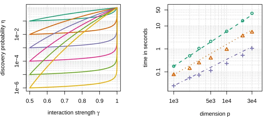
One of the surprising outcomes of our theoretical analysis is extent of the suboptimality of Gaussian random projections, which whilst they suffice for the conclusion of the Johnson– Lindenstrauss Lemma, are not well-suited for our purposes here (see Theorem 1). We can explicitly compute the probability of retaining an interaction of strength γ in E1 for both dense Gaussian projections ξGauss and minimal subsamplingξminimal given an equal
computational budget. We consider various values of p ranging from 10 up to 106 and we fix n = 1000. We set L = 1 and select other parameters of the algorithms to ensure the average size of E1 is equal to p in the setting when all interaction strengths are equal to 0.5. Specifically we make the following choices.
• ξGauss: the close pairs thresholdτ ≥0 is the 1/p–quantile of the distribution of|W|
when W ∼N(0,0.5n).
• ξminimal: the subsample size M =dlog(1/p)/log(0.5)e.
We then plot the probabilityη of discovering an interaction of strengthγ, as a function of
γ for different values of p (Figure 3). Forξminimal,η is given in equation (11). For ξGauss, η is the 1/p–quantile of the distribution of |W|when W ∼N(0, n(1−γ)).
5.2 Scaling
In this experiment we test how the xyz algorithm scales on a simple test example as we increase the dimension p. We generate dataX ∈ Rn×p with each entry sampled
indepen-dently uniformly from {−1,1}. We do this for different values of p, ranging from 1000 to 30 000: this way for the largest p considered there are more than 400 million possible interactions. Then for each X we construct response vectors Y such that only the pair (1,2) is a strong interaction with an interaction strength taking values in {0.7,0.8,0.9}. Through this construction, if nis large enough, all the pairs except (1,2) will have an in-teraction strength around 0.5, and very few will have one above 0.55. We thus set M so that γ0 = p−1/M ≈ 0.55. Since the only strong interaction is (1,2), we set γ =γ12 Each data set configuration determined by pand γ12 is simulated 300 times and we measure the time it takes xyz to find the pair (1,2). In Figure 3 we plot the average run time against the dimension pwith the different choices forγ12 highlighted in different colours.
Theorem 2 indicates that the run time should be of the order np1+log(γ)/log(γ0). We see
interaction strength γ
disco
v
er
y probability
η
0.5 0.6 0.7 0.8 0.9 1
1e−6
1e−4
1e−2
dimension p
time in seconds ● ●
● ●
● ●
●
1e3 5e3 1e4 3e4
0.1
1
10
50
Figure 3: Left panel: Discovery probability as a function of γ for different values of
p∈ {101, . . . ,106}(colours decreasing inpfrom yellowp= 106 to greenp= 10). The lower
lines correspond to the dense Gaussian projections, the upper lines to minimal subsampling. It can be seen that the discovery probability for minimal subsampling is much higher (up to factor 104) than for Gaussian projections. Right panel: Time to discover the interaction pair as a function of the data set dimensionp. Lines correspond to the theoretical prediction (with the intercept chosen based on the data points) and symbols give the actual measured run time. Colour coding: green γ = 0.7, orange γ= 0.8 and purple γ = 0.9.
5.3 Run on SNP data
In the next experiment we compare the performance of xyz to its closest competitors on a real data set. For each method we measure the time it takes to discover strong interactions. We consider the LURIC data set (Winkelmann et al., 2001), which contains data of patients that were hospitalised for coronary angiography. We use a preprocessed version of the data set that is made up ofn= 859 observations and 687 253 predictors. The data set is binary. The responseYindicates coronary disease (1 corresponding to affected and−1 healthy) and
X contains Single Nucleotide Polymorphisms (SNPs) which are variations of base-pairs on DNA. The response vectorY is strongly unbalanced: there are 681 affected cases (Yi = 1)
and 178 unaffected (Yi =−1).
To get a contrast of the performance of xyz we compare it to epiq (Arkin et al., 2014), another method for fast high-dimensional interaction search. In order for epiq to detect interactions it needs to assume the model
Yi=αj∗k∗Xij∗Xik∗+εi, (19)
whereεi ∼ N(0, σ2). It then searches for interactions by considering the test statistics
Tjk = (RT(Y◦Xj))(RTXk)
that E(Tjk) =YT(Xj ◦Xk). To maximise the inner product on the right, epiq considers
pairs where Tjk2 is large by looking at pairs where both (RT(Y◦Xj))2 and (RTXk)2 are large. While the approach ofepiq is somewhat related toxyz, there are no bounds available for the time it takes to find strong interactions.
We also compare both methods to a naive approach where we subsample a fixed number of interactions uniformly at random, and retain the strongest one. We refer to this asnaive search.
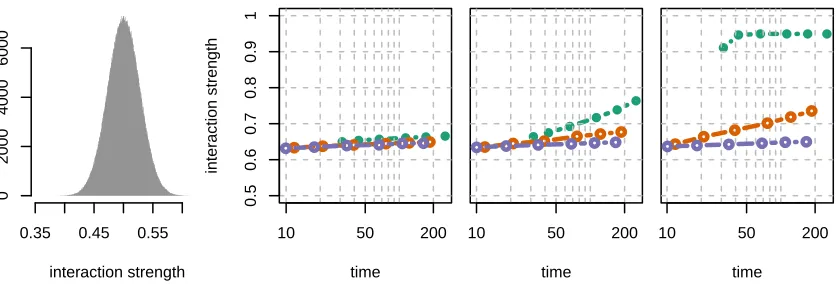
At fixed time intervals we check for the strongest interaction found so far with all three methods. We plot the interaction strength as a function of the computational time (Figure 4). All three methods eventually discover interactions of very similar strength and it would be a hasty judgement to say whether one significantly outperforms the others. xyz nevertheless discovers the strongest interactions on average for a fixed run time compared to the other two approaches. To get a clearer picture we run two additional experiments on a slight modification of the LURIC data set. We implant artificial interactions where we set the strength toγ12= 0.8 and another example withγ12= 0.9. In these two experiments xyz clearly outperforms all other methods considered (Figure 4; panels 3 and 4). Besides xyz being the fastest at interaction search, it also offers a probabilistic guarantee that there are no strong interactions left in the data. This guarantee comes out of Theorem 2. To run xyz we have to calculate the optimal subsample size (13) for use of minimal subsampling:
M∗= arg min
M∈N
− 1
log(1−γM)
M p+plog(p) +nX
j,k
γjkM
= 21.
The sum in this optimisation can be approximated by uniformly sampling over pairs. As-sume we have an interaction pair (j∗, k∗) with interaction strength γj∗k∗ = 0.85 and say the rest of the pairs (j, k) have an interaction strength of no more than γjk ≤ 0.55. The
probability that we discover this pair in one run (L = 1) of the xyz algorithm is γ21
j∗k∗. Therefore the probability of missing this pair afterL= 100 runs is given by
(1−γj21∗k∗)L≈0.03.
Note that the number of possible interactions is p(p−1)/2≈1011. The whole search took 280 seconds. Naive search offers a similar guarantee, however it is extremely weak. The probability of not discovering the pair after drawingpLsamples (withL= 100) is bounded by [1−2/{p(p−1)}]Lp ≈ 0.999. If we consider the run time guarantee from Theorem 2,
the dominating term in the complexity of xyz in terms of pis
p1+
log(0.85)
log(0.55) ≈p1.27.
interaction strength 0.35 0.45 0.55
0
2000
4000
6000
● ● ● ● ● ●
time
inter
action strength
● ● ● ● ● ● ● ● ● ● ● ●
0.5
0.6
0.7
0.8
0.9
1
10 50 200
● ● ●
● ●
●
time
● ● ●
● ● ● ● ● ● ● ● ●
10 50 200
●
● ● ● ● ●
time
● ● ● ●
● ●
● ● ● ● ● ●
10 50 200
Figure 4: Left: Histogram of interaction strength of 106 interaction pairs, sampled at random from the more than 1011 existing pairs from the LURIC data set. The right three panels show the interaction strength of the discovered pairs as a function of the computation time for xyz (green), epiq (orange) and naive search (purple). The first panel gives results on the the original LURIC data set, and the second and third (rightmost) panels show results with an implanted interaction with strengthsγ12= 0.8 andγ12= 0.95 respectively. It can be clearly seen thatxyz outperforms its competitors by a large margin.
5.4 Regression on artificial data
In this section we demonstrate the capabilities of xyz in interaction search for continuous data as explained in Section 3. We simulate two different models of the form (15):
Yi =µ+
p X
j=1
Xijβj+
p X
k=1
k−1
X
j=1
XijXikθjk+εi.
We consider three settings. For all three settings we haven= 1000. We letp∈ {250,500,750,
1000}. Each row of X is generated i.i.d. as N(0,Σ). The magnitudes of both the main and interaction effects are chosen uniformly from the interval [2,6] (20 main effects and 10 interaction effects) and we set εi ∼ N(0,1). The three settings we consider are as follows.
1. Σ=I ∈Rp×p, we generate a hierarchical model: θjk 6= 0⇒ βj 6= 0 and βk6= 0. We
first sample the main effects and then pick interaction effects uniformly from the pairs of main effects.
2. Σ=I∈Rp×p, we generate a strictly non-hierarchical model: θjk 6= 0 ⇒ βj = 0 and βk = 0. We first sample the main effects and then pick interaction effects uniformly
from all pairs excluding main effects as coordinates.
a substantial number of variables strongly correlated to Xj (There is usually around
10 variables with a correlation of above 0.9). Such a correlation structure will make it easier to detect pairs of variables whose product can serve as strong predictor ofY, even though it has not been included in the construction ofY.
We run three different procedures to estimate the main and interaction effects.
• Two-stage Lasso: We fit the Lasso to the data, and then run the Lasso once more on an augmented design matrix containing interactions between all selected main effects. Complexity analysis of the Least Angle Regression (LARS) algorithm (Efron et al., 2004) suggests the computational cost would be O(npmin(n, p)), making the procedure very efficient. However, as the results show, it struggles in situations such as that given by model 2, where a main effects regression will fail to select variables involved in strong interactions.
• Lasso with all interactions: Building the full interaction matrix and computing the standard Lasso on this augmented data matrix. Analysis of the LARS algorithm would suggest the computational complexity would be in the orderO(np2min(n, p2)). Nevertheless, for small p, this approach is feasible.
• xyz: This is Algorithm 3; we set the parameterL to be √p in order to target the strong interactions.
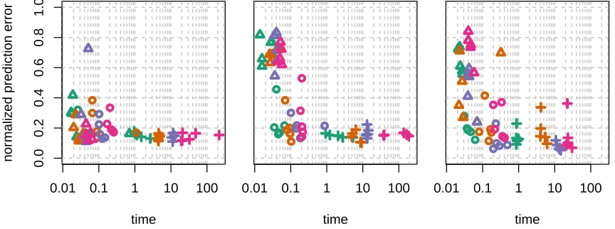
The experiment (seen in Figure 5) shows thatxyz enjoys the favourable properties of both its competitors: it is as fast as the two-stage Lasso that gives an almost linear run time inp, and it is about as accurate as the estimator calculated from screening all pairs (brute-force).
0.0
0.2
0.4
0.6
0.8
1.0
nor
maliz
ed prediction error
0.01 0.1 1 10 100
● ●●● ●
●
● ● ● ●
● ● ●
● ●
● ●
● ●●
time
0.01 0.1 1 10 100
●● ● ●
●
● ●
● ● ● ●
● ● ● ●
●
● ● ●
●
time
0.01 0.1 1 10 100
● ● ●● ●
● ●
●
● ● ● ●
●● ● ●
● ● ●
●
time
5.5 Regression on real data
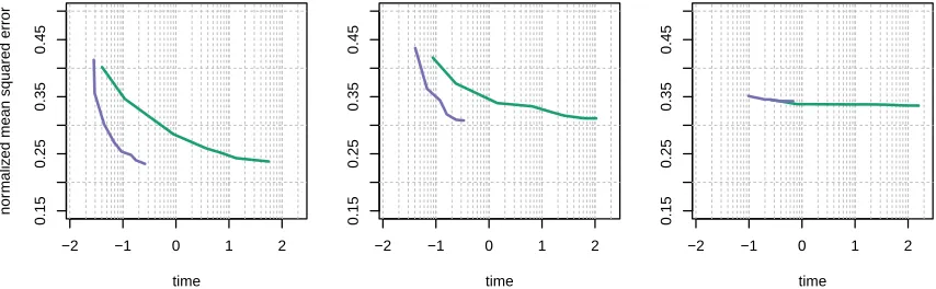
Here we runxyz regression on continuous real data sets where the ground truth is unknown. On each data set we pick at random p= 2000 variables and run xyz and the Lasso imple-mented in glmnet with all interactions included. We subsample an increasing number of variables to vary the difficulty of the regression problem. For each sample we measure the run time and the normalized out of sample squared `22 error:
kYtest−Xtestβˆ−W˜ testθˆk22
kYtestk22
.
Experiments are run on the following three different data sets:
• Riboflavin: The Riboflavin production data set (B¨uhlmann et al., 2014) contains
n= 71 samples andp= 4088 predictors (gene-expressions). The responseY and the designX are both continuous.
• Kemmeren: The Kemmeren (Kemmeren and et al., 2014) data set records knock-outs ofp= 6170 genes. The dataX is continuous. We sample Y randomly from the genes not present in the subsample taken fromX.
• Climate: The climate data set from the CNRM model from the CMIP5 model ensemble (Knutti et al., 2013) simulates the temperature of points on the northern hemisphere which is recorded inX. The response Y simulates the temperature on a random position on the southern hemisphere. The data containsn= 231 observations.
−2 −1 0 1 2
0.15
0.25
0.35
0.45
time
nor
maliz
ed mean squared error
−2 −1 0 1 2
0.15
0.25
0.35
0.45
time
−2 −1 0 1 2
0.15
0.25
0.35
0.45
time
Figure 6: From left to right column the experiments correspond to Riboflavin, Kemmeren and Climate. The y-axis depicts the normalized squared error and the x-axis records the run time in seconds on the log10scale. It can be seen thatxyz (purple) offers clear computational advantages while giving similar level of prediction error to the Lasso fitted to all interactions as implemented inglmnet(green).
6. Discussion
Table of frequently used notation
n, p number of observations and number of variables
X,Y predictor matrix and response vector
Xj jth variable / column of X
β,θ coefficients of main effects and interaction effects
γjk interaction strength of the pair (j, k) G distribution of projection
M subsample size
R projection vector
L number of projections
τ, γ close pairs threshold and interaction strength threshold Ξ set of all configurations of the xyz algorithm, the elements
of this set are denoted byξ
η probability that a given interaction is present in the output of the xyz algorithm
˜
X binarized version of X
W predictor matrix containing all possible interaction pairs
Appendix A
Here we include proofs that were omitted earlier.
Proof of Theorem 1
In the following, we fix the following notation for convenience: Ψ = Ξminimal, Ψ(η) = Ξminimal(η), Ξ = Ξsubsample, Ξ(η) = Ξsubsample(η).
Note that both Ψ(η) and Ξ(η) depend onF though this is suppressed in the notation. Also define Ξall = Ξ∪Ξdense and Ξall(η) = Ξ(η)∪Ξdense(η). We will reference the parameters levels contained inξ∈Ξall asξLandξτ. Ifξ∈Ξ then we will writeξM for the distribution
of the subsample sizeM.
If we let V denote the complexity of the search for τ-close pairs, similarly to (10) we have that
T(ξ) =c1np+L(c2EξM p+EξV +c3nEξ|E1|), (20)
wherec1, c2, c3 are constants. Supposeψ∈Ψ and ξ∈Ξ haveEξ|E1|=Eψ|E1|. Then since searching for τ-close pairs is at least as computationally difficult as finding equal pairs we know thatEξV ≥EψV.
Similarly for ξ∈Ξdense we have
For ξ∈Ξall, define
α(ξ) =Eξ|E1|/p2, β(ξ) =Pξ((j∗, k∗)∈I1)
whereI1 is the set of candidate interactionsI when L= 1. Note that
Pξ((j∗, k∗)∈I) = 1− {1−β(ξ)}ξL.
Thus anyξ∈Ξall(η) with T(ξ) minimal must haveξLas the smallest Lsuch that 1− {1− β(ξ)}ξL≥η, whence
ξL=dlog(1−η)/log{1−β(ξ)}e. (22)
Note that β(ξ) does not depend on ξL, so the above equation completely determines the
optimal choice ofLonce other parameters have been fixed. We will therefore henceforth as-sume thatLhas been chosen this way so that the discovery probability of all the algorithms is at least η.
The proofs of (8) and (9) are contained in Lemmas 12 and 13 respectively. The proof of (7) is more involved and proceeds by establishing a Neyman–Pearson type lemma (Lem-mas 10 and 11) showing that given a constraint on the ‘size’ α that is sufficiently small, minimal subsampling enjoys maximal ‘power’β. To complete the argument, we show that any sequence of algorithms with size α remaining constant as p → ∞ cannot have a sub-quadratic complexity, whilst Lemma 12 attests that in contrast minimal subsampling does have subquadratic complexity under the assumptions of the theorem. Several auxiliary technical lemmas are collected in Section 6
Our proofs Lemmas 10 and 11 make use of the following bound on a quantity related to the ratio of the size to the power of minimal subsampling.
Lemma 9 Suppose ψ∈ Ψhas distribution for M placing mass on M and M+ 1. Under the assumptions of Theorem 1,
α(ψ)
γM
1
≤ 2
1−ρ
1
M+ 1.
Proof We have
α(ψ)
γM
1
≤ 1
p2
X
j,k
(γjk/γ1)M ≤
c0
p +
nγ1−1
X
i=0
i
nγ1
M
fn(i/n).
Now the sum on the RHS is maximised over fn obeying constraints (A1) and (A2) in the
following way. Ifργ1n > γ1n−1 then fn places all available mass on γ1−1/n. Otherwise
fn should be as close to constant as possible ondργ1ne/n, . . . ,(γ1n−1)/n, and zero below
dργ1ne/n. In both cases it can be seen that
nγ1−1
X
i=0
i
nγ1
M
fn(i/n)≤
2 1−ρ
Z 1 (1+ρ)/2
xMdx≤ 2
1−ρ
1
M + 1.
Lemma 10 Let Ξ0 be the set of ξ ∈ Ξ such that ξM places mass only on a single M, so
the subsample size is not randomised. There exists an α0 independent ofnsuch that for all
α0≤α0, we have
sup
ψ∈Ψ:α(ψ)≤α0
β(ψ) = sup
ξ∈Ξ0:α(ξ)≤α0
β(ξ).
Moreover the suprema are achieved.
Proof Each ξ ∈Ξ0 is parametrised by its close pairs thresholdτ and subsample size M. Given aξ ∈Ξ0 with parameter values τ and M we compute α(ξ) as follows. Note that by replacing the thresholdτ byτ /2, we may assume thatXandZhave entries in{−1/2,1/2}. ThusXj−Zk has components in{−1,0,1}. LetJjk be the number of non-zero components
of (Ximj −Zimk)
M
m=1. Then Jjk ∼Binom(M,1−γjk). Thus
P M X m=1
Dm(Ximj−Zimk)
≤τ
=P(Jjk = 0) + M X r=1 P r X m=1 Dm ≤τ
P(Jjk =r),
noting that Dm d
= −Dm. By Lemma 14 we know there exists an a > 0 such that for all τ ≤a√M the RHS is bounded below by
γjkM +
M X
r=r0
c√1τ
r
M r
γjkM−r(1−γjk)r (23)
forM sufficiently large. Here the constants a, c1>0 andr0∈Ndepend only onF.
Consider τ > a√M. In this case, for r≤M sufficiently large we have by Lemma 14
P r X m=1 Dm ≤τ ≥P r X m=1 Dm
≤a√r
≥c1a.
However then forM sufficiently large,
P(Jjk = 0) + M X r=1 P r X m=1 Dm ≤τ
P(Jjk =r)≥c1a/2,
so α(ξ) ≥c1a/2. Note also that we must have α0 ≥α(ξ) ≥γlM, so M ≥log(α0)/log(γl).
Thus by choosing 0 < α0 < c1a/2 sufficiently small, we can rule out τ > a
√
M and so we henceforth assume thatτ ≤a√M, and thatM is sufficiently large such that (23) holds for all (j, k).
We have
α(ξ)≥ 1
p2
X
j,k
γjkM+τ
M X
r=r0
c1 √ r M r
γjkM−r(1−γjk)r
. (24)
Similarly we have
β(ξ)≤γ1M +τ
M X r=1 c2 √ r M r
Now substituting the upper bound on τ implied by (24) into (25), we get
β(ξ)≤γ1M +QM
α(ξ)− 1
p2
X
j,k
γjkM
where
QM =
c2PMr=1r−1/2
M r
γ1M−r(1−γ1)r
c1p−2Pj,kPr=r0r−1/2 Mr
γjkM−r(1−γjk)r
.
Now by Lemma 15, for M sufficiently large and some constant Qwe have
QM ≤Q
√
1−γ1
P j,k
p
1−γjk/p2
≤Q.
Thus
β(ξ)≤γ1M +Q
α(ξ)− 1
p2
X
j,k
γjkM
(26)
for all M sufficiently large. Now givenα0, letM0 be such that 1
p2
X
j,k
γM0
jk ≥α0 ≥
1
p2
X
j,k
γM0+1
jk .
Consider the minimal subsampling algorithm ψ that chooses subsample size as either M0 orM0+ 1 with probabilitiesband 1−b such that
α(ψ) = 1
p2
X
j,k
{bγM0
jk + (1−b)γ M0+1
jk }=α0. Then we have β(ψ) = bγM0
1 + (1−b)γM1 0+1. Now supposeξ ∈Ξ0 has α(ξ)≤α0. Then in particular M ≥M0+ 1. We first examine the case whereM =M0+ 1. Then
1
γM0
1
{β(ψ)−β(ξ)} ≥b+ (1−b)γ1−γ1−
Q
γM0
1
α0−
1
p2
X
j,k
γM0+1
j,k
=b+ (1−b)γ1−γ1−
aQ
γM0
1 1
p2
X
j,k
(γM0 j,k −γ
M0+1 j,k )
≥b
(1−γu)−
2Q
1−ρ
1
M0+ 1
,
using Lemma 9 in the final line. Note this is non-negative for M0 sufficiently large. When
M ≥M0+ 2 we instead have
β(ξ)
β(ψ) ≤
β(ξ)
γM0+1
1
≤γ1+ 2Q
γ1(1−ρ)
1
M0+ 1
≤γu+
2Q
γl(1−ρ)
1
M0+ 1
<1
Lemma 11 There exists an α0 independent of n such that for all α0 ≤α0, we have sup
ψ∈Ψ:α(ψ)≤α0
β(ψ) = sup
ξ∈Ξ:α(ξ)≤α0
β(ξ).
Moreover the suprema are achieved.
Proof With a slight abuse of notation, write ξ(M0, τ0) for the element of ξ ∈Ξ that fixes
M =M0 and τ =τ0. Using the notation of Lemma 10, define functionf : [0,1]→[0,1] by
f(α0) = sup
ξ∈Ξ0:α(ξ)≤α0
β(ξ).
Note that forξ ∈Ξ we have
β(ξ)≤EM∼ξMf[α{ξ(M, ξτ)}]. (27)
Now by Lemma 10 we know there exists α0 (depending onF) such that on [0, α0],f is the linear interpolation of points
1
p2
X
j,k
γj,kM, γM1
∞
M=1
.
We claim thatf is concave on [0, α0]. Indeed, it suffices to show that the slopes of the suc-cessive linear interpolants are decreasing in this region, or equivalently that their reciprocals are increasing. We have
1
p2
X
j,k
γjkM+1−γjkM
γ1M+1−γ1M =
1
p2
X
j,k
γj,k
γ1
M
γjk−1
γ1−1
(28)
which increases asM decreases, thus proving the claim.
Note also that the RHS of (28) is at most α(ψ)/{(1−γu)γM1 } when ψ has subsample size fixed atM. Thus by Lemma 9 we see the derivatives of the linear interpolants approach infinity as they get closer to the origin. This implies the existence of an 0< α1 < α0 such that −sup ∂(−f)(α1)
≥ {1−f(α1)}/(α0−α1), where ∂(−f)(α1) denotes the subdiffer-ential of the function−f atα1. We may therefore invoke Lemma 16 to conclude that forξ
withα(ξ)≤α1
EM∼ξMf[α{ξ(M, ξτ)}]≤f[EM∼ξMα{ξ(M, ξτ)}] =f(α(ξ))≤f(α1) = max
ψ∈Ψ:α(ψ)≤α1
β(ψ).
Combining with (27) gives the result.
The next lemma establishes subquadratic complexity of minimal subsampling.
Lemma 12 Under the assumptions of Theorem 1, we have infψ∈Ψ(η)T(ψ)/(np2)→0.
Proof Letψ∈Ψ be such thatψM places all mass on M. We have thatβ(ψ) =γ1M. Thus using the inequality −x≤log(1−x) for x∈(0,1), we have
Lemma 9 gives an upper bound onψLEψE1. Note that EψV =O(plog(p)). Thus ignoring
constant factors, we have
T(ψ)/(np2)≤ M+ log(p)
γM
1 np
+ 1
M + 1.
Taking M =log(1/√p)/log(γ1)
then ensures T(ψ)/(np2)→0.
Lemma 13 Let ξ∈Ξdense. There exists c >0 andn0 ∈N such that for all n≥n0, inf
ξ∈ΞdenseT(ξ)/(np
2)> c.
Proof Eachξ∈Ξdenseis parametrised by its close pairs thresholdτ. Given aξ ∈Ξdense(F) with close pairs threshold τ we compute α(ξ) as follows. Similarly to Lemma 10 we may assume without loss of generality thatXandZhave entries in{−1/2,1/2}soXj−Zkhas components in{−1,0,1}. Since Ri
d
=−Ri asF ∈ F, we have
P n X i=1
Ri(Xij−Zik)
≤τ =P
n(1−γjk) X i=1 Ri ≤τ .
We now use Lemma 14. Forn(1−γu) sufficiently large, whenτ ≤a
√
nthe RHS is bounded below by
c1τ
p
n(1−γjk)
.
Here constant a, c1>0 also depend only on F. Thus
α(ξ)≥ 1
p2
X
j,k
c1τ
p
n(1−γjk)
≥c1τ /
√
n. (29)
Similarly we have
β(ξ)≤ p c2τ
n(1−γ1)
. (30)
Note that from (29), when τ > a√n we have α(ξ) ≥ c1a. Thus from (21) we know there existsn0 such that for alln≥n0, we have
inf
ξ∈Ξdense(η):ξτ>a √
nT(ξ)/(np
2)≥ inf
ξ∈Ξdense(η):ξτ>a √
nξLα(ξ)
≥ξLc1a >0. (31)
We therefore need only consider the case where τ ≤a√nand whereα(ξ)→0. Substituting the upper bound on τ implied by (29) into (30), we get
β(ξ)≤α(ξ) c2
c1
√