ADMMBO: Bayesian Optimization with Unknown
Constraints using ADMM
Setareh Ariafar [email protected]
Electrical and Computer Engineering Department Northeastern University
Boston, MA 02115, USA
Jaume Coll-Font [email protected]
Computational radiology Laboratory Boston Children’s Hospital
Boston, MA 02115, USA
Dana Brooks [email protected]
Electrical and Computer Engineering Department Northeastern University
Boston, MA 02115, USA
Jennifer Dy [email protected]
Electrical and Computer Engineering Department Northeastern University
Boston, MA 02115, USA
Editor:Bayesian Optimization Special Issue
Abstract
There exist many problems in science and engineering that involve optimization of an un-known or partially unun-known objective function. Recently, Bayesian Optimization (BO) has emerged as a powerful tool for solving optimization problems whose objective functions are only available as a black box and are expensive to evaluate. Many practical problems, however, involve optimization of an unknown objective function subject to unknown con-straints. This is an important yet challenging problem for which, unlike optimizing an un-known function, existing methods face several limitations. In this paper, we present a novel constrained Bayesian optimization framework to optimize an unknown objective function subject to unknown constraints. We introduce an equivalent optimization by augmenting the objective function with constraints, introducing auxiliary variables for each constraint, and forcing the new variables to be equal to the main variable. Building on the Alternating Direction Method of Multipliers (ADMM) algorithm, we propose ADMM-Bayesian Opti-mization (ADMMBO) to solve the problem in an iterative fashion. Our framework leads to multiple unconstrained subproblems with unknown objective functions, which we then solve via BO. Our method resolves several challenges of state-of-the-art techniques: it can start from infeasible points, is insensitive to initialization, can efficiently handle ‘decoupled problems’ and has a concrete stopping criterion. Extensive experiments on a number of challenging BO benchmark problems show that our proposed approach outperforms the state-of-the-art methods in terms of the speed of obtaining a feasible solution and con-vergence to the global optimum as well as minimizing the number of total evaluations of unknown objective and constraints functions.
c
Keywords: Bayesian Optimization, Gaussian Processes, ADMM, Expected Improvement
1. Introduction
Bayesian optimization (BO) has been shown to be a powerful tool for solving optimization problems whose objective functions are unknown and expensive to evaluate (Brochu et al., 2010a; Martinez-Cantin et al., 2007; Hutter et al., 2011; Torn and Zilinskas, 1989). For example, in drug design (Azimi et al., 2012; Scott, 2010; Brochu et al., 2010b), where the goal is to maximize the efficacy of a drug, the evaluation of the objective function, i.e., drug efficacy, across multiple drug formulations requires producing and testing new drugs, which would be subject to resource and cost limitations. As another example, minimizing the validation error of a machine learning model, such as hyperparameter tuning of a deep neural network (LeCun et al., 2015), involves many evaluations of the objective function, i.e., the validation error, where each evaluation requires training and evaluating a new model (Bergstra et al., 2011; Hoffman et al., 2014; Snoek et al., 2012; Swersky et al., 2013).
In many real-world problems, the desired solution, in addition to optimizing the objective function, must satisfy constraints that are also unknown and expensive to evaluate (Shahri-ari et al., 2016). For example, in the drug design problem, the goal is often to maximize the drug efficacy while limiting its side effects. In the hyperparameter tuning problem in machine learning, the optimal hyperparameters not only must minimize the validation error, but also must ensure that the prediction time of the learned model is sufficiently short. The majority of existing work on BO has focused on the unknown-objective problem (Jones et al., 1998; Kushner, 1964; Lizotte, 2008; Jones, 2001; Hern´andez-Lobato et al., 2014; Cox and John, 1992; Wu et al., 2017), while only a few recent reports have addressed the problem in the unknown-objective unknown-constraint setting (Snoek, 2013; Gelbart et al., 2014; Gardner et al., 2014; Bernardo et al., 2011; Hern´andez-Lobato et al., 2015; Picheny et al., 2016; Gramacy et al., 2016; Picheny, 2014), (see Section 4 for a review).
1.1. Existing Challenges & Paper Contributions
the model and is often much cheaper than evaluating the validation error. Thus, methods that require joint evaluation of all unknown functions, including EIC, IECI, EVR, ALBO, and Slack-AL could increase the overall cost of solving decoupled problems more than might be necessary. Third, the majority of existing methods, including IECI, EVR, ALBO and Predictive Entropy Search with Constraints (PESC) (Hern´andez-Lobato et al., 2015), do not have closed form expressions for the so-called ‘acquisition function’, which is a key step in the BO algorithm. Thus, these methods need to approximate the acquisition function, typically via algorithms such as Expectation Propagation (Minka, 2001) or Monte-Carlo Sampling (Picheny et al., 2013), which often suffer from implementation difficulty and slow execution time, or may cause instabilities (Picheny et al., 2016; Gelbart, 2015). Finally, most of the BO methods fix a computational budget in terms of either wall-clock time or the number of function evaluations, and stop when the budget is exhausted. However, this budget is an additional parameter which must be hand tuned, and the performance of the BO method typically is highly dependent on it. A value that is too small may result in missing easy improvement while one that is too large might incur additional cost for an insignificant gain. Thus, having an automatic stopping criterion is highly desirable while many BO methods, including EIC, IECI, EVR and PESC, lack such a criterion.
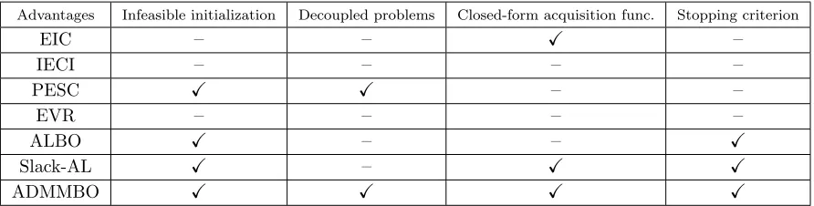
In this paper, we propose a novel constrained BO framework for optimizing an unknown objective function subject to unknown constraints that resolves all the aforementioned chal-lenges. First, we reformulate the problem into an equivalent unconstrained optimization. Since the joint (Bayesian) optimization of the unconstrained problem over the unknown ob-jective function and unknown augmented constraints is challenging, we introduce auxiliary variables, one per constraint, and then force these variables to be equal to the the original variable, resulting in an equivalent constrained formulation, where the constraints are now known. The new formulation allows to perform the (Bayesian) optimization over each term independently, decoupling the objective function optimization from constraint satisfaction. To efficiently solve our proposed optimization, we adopt the Alternating Direction Method of Multipliers (ADMM) framework (Boyd et al., 2011; Hong and Luo, 2017; Parikh et al., 2014), which leads to solving an ‘optimality subproblem’, and a ‘feasibility subproblem’ for each constraint, at each iteration. The optimality subproblem minimizes the objective function close to current solutions of the feasibility subproblems, while each feasibility sub-problem searches for a feasible solution of its constraint close to the current solution of the optimality subproblem. Our framework, which we call Alternating Direction Method of Multipliers for Bayesian Optimization (ADMMBO), provides the following advantages compared to the state-of-the-art methods (see Table 1 for a summary).
– Unlike many existing methods, ADMMBO can start from an infeasible initial point and gradually move towards a feasible point via solving the feasibility subproblems.
– Due to its separation of the optimizations over each expensive to evaluate function, i.e., objective function and each constraint, ADMMBO can handle decoupled problems efficiently, without requiring joint evaluation of all such functions at each candidate point.
Advantages Infeasible initialization Decoupled problems Closed-form acquisition func. Stopping criterion
EIC – – X –
IECI – – – –
PESC X X – –
EVR – – – –
ALBO X – – X
Slack-AL X – X X
ADMMBO X X X X
Table 1: Advantages of ADMMBO with respect to the state-of-the-art methods.
–ADMMBO offers a well-defined stopping criterion, inherited from ADMM, which in prac-tice avoids unnecessary function evaluations. The stopping criterion is satisfied when the solutions of the optimality and feasibility subproblems converge to each other.
– Our experiments empirically show that ADMMBO achieves good solutions significantly faster than the state-of-the-art methods, is relatively insensitive to initialization, and re-quires fewer function evaluations to find desirable solutions. Moreover, our results suggest that ADMMBO’s performance does not depend on whether the optimal solution lies on the boundary of or inside the feasible region, and is also insensitive to the relative volume of the feasibility region.
1.2. Paper Organization
In Section 2, we review both BO and the ADMM algorithm that we build upon. We motivate and introduce our proposed reformulation of the constrained problem and present our ADMMBO algorithm to solve this reformulated optimization in Section 3. In Section 4, we discuss existing related work on constrained BO that handles unknown-objective unknown-constraint optimization problems. We present experimental results on synthetic and real data in Section 5. Finally, in Section 6, we discuss our results and open avenues for future research and conclude the paper.
2. Background
In this section, we review the underlying components of our proposed method: Bayesian Optimization in its standard settings, with a focus on EI as the acquisition function, and the ADMM algorithm.
2.1. Bayesian Optimization
Bayesian optimization (Shahriari et al., 2016; Brochu et al., 2010b) addresses the problem of finding a global minimum (or maximum), x∗, of an objective function f(x) over a bounded box B ∈ Rd, where f is unknown but available to evaluate pointwise via computationally
costly queries. Thus, the goal is to find x∗ with as few evaluations of f(x) as possible. Given a collection of initial points in B and their observed objective values, denoted by
F = { xl, f(xl)
}n
evaluate the corresponding objective value at iterationl+ 1. More specifically, to findxl+1, BO first assumes a prior probability model for the unknown functionf, denoted bypf(x), and then uses the observed data, F, to update the posterior probability pf(x)|F
. This posterior is then used to build anacquisition function, denoted byα(x), which provides an estimate of theoptimization usefulness of any candidate pointx∈ B if it is chosen asxl+1 for the next function evaluation. In contrast to f(x), the acquisition function α(x) has a known form and can be maximized over x∈ B, using analytical or numerical optimization techniques. The optimum of the acquisition function provides a recommendation for xl+1 that is used to evaluatef(xl+1) and then to update the dataF accordingly. BO iteratively repeats this process, guiding the search towards sampling a global minimizer of f.
Many BO methods assume that the unknown function f(x) is a Lipschitz continuous bounded function over B, and then model pf(x) as a Gaussian Process (GP) (Moˇckus, 1975; Jones et al., 1998; Hern´andez-Lobato et al., 2014; Kushner, 1964; Cox and John, 1992). GPs are non-parametric Bayesian models which are widely used in the Bayesian optimiza-tion literature since they provide a flexible fit for modeling unknown funcoptimiza-tions. Moreover given GP models, some acquisition functions give closed-form expressions, which can be ef-ficiently optimized with numerical optimization techniques (Rasmussen and Williams, 2006; Houlsby et al., 2012). As an example, which we will then employ in the exposition of our method below, we describe a popular acquisition function called Expected Improvement (Jones et al., 1998; Brochu et al., 2010b).
Given dataF, letf+ denote the best objective value achieved by the points inF. Then the improvement of any given pointx, denoted byI(x), corresponds to the improvement of f(x) relative to f+, i.e., I(x), max(0, f+−f(x)). An efficient strategy in BO would be to choose the next candidate for function evaluation by finding a point x which offers the largest improvement (Jones et al., 1998). However, since f(x) is unknown and expensive to evaluate pointwise, it is difficult to calculate improvementI(x). Alternatively, Expected Improvement ofx, denoted byEI(x), is an acquisition function which computes the expec-tation ofI(x) with respect top
f(x)|F
. Moˇckus (1975); Jones et al. (1998); Brochu et al. (2010b) has shown that assuming a GP model for pf(x), the Expected Improvement can be computed using the closed-form expression
EI(x) =Ef|F
I(x)=σf(x)
"
mf(x)−f+
σf(x)
Φ mf(x)−f + σf(x)
+φ mf(x)−f + σf(x)
#
, (1)
where the expectation is computed with respect to the posterior probability p[f(x)|F]. Here, Φ(·) denotes the normal cumulative distribution function,φ(·) is the standard normal probability density function, and mf(x) and σf(x) are the posterior mean and standard
2.2. Alternating Direction Method of Multipliers (ADMM) Optimization
Our reformulation of the optimization of an unknown-objective unknown-constraint prob-lem allows us to build a framework based on a popular numerical optimization technique, ADMM (Boyd et al., 2011; Hong and Luo, 2017; Parikh et al., 2014), which we briefly review here. Consider the problem of minimizing f(x) +g(x) with respect to x, where x ∈ Rd and f, g : Rd → R. Specifically, consider the case where separately minimizing
f(x) and g(x) is relatively easy, while optimizing their sum is challenging. For example in the Least Absolute Shrinkage and Selection Operator (LASSO) problem (Tibshirani, 1996; Mota et al., 2013), we are interested in minimizing kAx−bk2
2+λkxk1 with respect to x, with an overdetermined dictionary,A. While each term can be easily minimized, it is much harder to minimize the sum of the two terms. ADMM is a powerful numerical optimization method which handles such cases (Boyd et al., 2011; Hong and Luo, 2017).
In order to minimize f(x) +g(x), ADMM first defines an auxiliary variablez ∈Rd for
the function g, and considers the following optimization, which is equivalent to the original minimization problem,
min
x,z f(x) +g(z) s.t. x=z. (2)
To solve (2), ADMM first builds the augmented Lagrangian function (ALF) for (2), where the ALF provides an unconstrained surrogate function for the constrained problem. Specif-ically, ALF augments the objective function of a constrained problem with terms penalizing the infeasibility of the constraints. These penalty terms include the product of the feasibility gap with a dual variable vector, also called a Lagrange multiplier vector, and the squared Euclidean norm of the feasibility gap. More specifically, ALF for (2) is given by
Lρ(x, z, y),f(x) +g(z) +yT(x−z) +
ρ 2 x−z
2
2, (3)
wherey∈Rddenotes the Lagrange multiplier vector corresponding to the constraint,x−z
is the feasibility gap, andρ is a positive penalty parameter.
Starting from an initial value fory, z, ADMM iteratively updates the values of variables x, y, zby minimizing the ALF, until convergence. Letxk, zk, ykdenote the values of variables at iteration k. At iteration k+ 1, ADMM solves two optimization problems, one over x while fixing z = zk and y = yk and one over z while fixing x = xk+1 and y = yk, and updates the Lagrange multiplier vector afterwards. More specifically, at iteration k+ 1, ADMM solves
xk+1= argmin
x
Lρ(x, zk, yk) = argmin x
f(x) + (yk)T(x−zk) +ρ 2 x−zk
2 2, zk+1= argmin
z
Lρ(xk+1, z, yk) = argmin z
g(z) + (yk)T(xk+1−z) + ρ 2
xk+1−z 2 2, yk+1 =yk+ρ(xk+1−zk+1).
(4)
The primal residual is defined as rk+1 , xk+1−zk+1, i.e., the gap between the main variable x and the auxiliary variable z, and the dual residual can be shown to be sk+1 ,
−ρ(zk+1 −zk) (Boyd et al., 2011; Hong and Luo, 2017). Assuming f and g are closed, proper and convex, and also that the unaugmented LagrangianLρ(x, z, y)−ρ2
x−z
yk → y∗ where p∗ is the optimal objective value of primal problem (2) and y∗ is the dual optimal point. The necessary and sufficient optimality conditions for the ADMM problem are primal feasibility and dual feasibility, and they are effecively met in practice when the `2-norm of both the primal and dual residuals of (2) fall below an appropriately small tolerance.
Boyd et al. (2011) shows that ADMM can be extended to problems optimizing sum of more than two functions. In this situation, ADMM defines a distinct auxiliary variable zi
for each additional functiongi, i= 1, . . . , N, and enforces each such variable to be equal to
the main variable x. The rest of the algorithm naturally follows. See (Boyd et al., 2011), chapter 7 for a detailed discussion.
3. Constrained Bayesian Optimization via ADMMBO
In this section, we describe our proposed framework, which we refer to as ADMMBO, for solving the Bayesian optimization problem under unknown constraints. More specifically, we consider the constrained optimization problem of
min
x∈B f(x)
s.t. ci(x)≤0, i= 1, . . . , N,
(5)
where, B ⊂ Rd is a bounded domain andf, c
i :Rd→ Rare unknown functions which can
be evaluated pointwise. However, such evaluations are expensive. Our goal is to determine a sampling procedure forxthat sequentially approaches a global optimum, x∗, with as few function queries from f and all ci’s as possible.
To tackle the problem, we first reformulate (5) into the unconstrained optimization
min
x∈B f(x) +
N
X
i=1
M1(ci(x)>0),
(6)
where 1(·) is an indicator function, which is one when its argument is true and is zero otherwise, andM is a positive constant (Boyd et al., 2011). For a sufficiently largeM, the constrained problem in (5) will be equivalent to the unconstrained one in (6).
Proposition 1. Given Lipschitz continuity off and compactness of B, f is bounded for every x in B. Let η` and ηu denote, respectively, the lower and upper bound of f, i.e.,
η` ≤f(x)≤ηu, ∀x∈ B. Assume the feasible region of (5) is non-empty. For M > ηu−η`,
the unconstrained optimization in (6) will be equivalent to (5).
Proof. LetJ(x) denote the value of the objective function of (6). For any infeasible point of
(5)xi∈ B, we haveJ(xi)≥η`+M, since the minimum value thatf can attain isη`and the
second term in (6) will be at least M, as xi is infeasible for at least one constraint. On the
other hand, for any feasible point xf ∈ B of (5), we have J(xf)≤ηu. Since M > ηu−η`,
we always have J(xf) < J(xi), hence (6) always finds a feasible solution, which makes the
A key observation in our proposed framework is that while jointly minimizing the objec-tive function in (6) is difficult, individually minimizing each term of the objecobjec-tive function using Bayesian optimization allows independent function evaluations for f and each ci.
More specifically, we can minimize f(x) with respect to x by assuming a GP model for pf(x)and using BO afterwards. Similarly, we can minimize 1(ci(x)>0) with respect to
x by assuming a GP model for pci(x)
and using it to build a Bernoulli random variable with parameter θi ,p
ci(x)>0
to represent 1(ci(x)>0), and then applying BO. In
con-trast, optimizing the entire objective function in (6) is difficult and also may require joint function evaluations for f and every ci. To take advantage of the simplicity of individually
optimizing each term in the objective function of (6), we introduce N auxiliary variables, one per constraint function, and consider the following optimization problem
min
x,z1,...,zN∈B
f(x) +
N
X
i=1
M1(ci(zi)>0)
s.t. x=zi, i= 1, . . . , N.
(7)
which clearly is equivalent to (6). Notice that in contrast to the objective unknown-constraint problem in (5), in (7) the equality unknown-constraints are known (deterministic) and only the objective function is unknown. Moreover, each of the unknown terms in the objective function of (7) is defined over a different variable, leading to a variable separation property which we will take advantage of. Next, we describe how ADMMBO combines Bayesian optimization with an ADMM-inspired framework to solve (7) efficiently.
3.1. ADMMBO Formulation
In this section, we describe our approach to combine the ADMM algorithm with BO steps to solve the proposed equivalent reformulation in (7). We first need to build the ALF for the optimization in (7), which is given by
Lρ(x, zi, yi) =f(x) + N
X
i=1 h
M 1(ci(zi)>0) +yiT(x−zi) +
ρ 2 x−zi
2 2 i
=f(x) +
N
X
i=1 h
M 1(ci(zi)>0) +
ρ 2
x−zi+
yi
ρ 2 2−
ρ 2 yi
2 2 i
,
(8)
where yi ∈ Rd is a Lagrange multiplier vector, and ρ is a positive penalty parameter.
More specifically, for (8), thekth ADMM iteration will become
xk+1= argmin
x∈B
f(x) +
N
X
i=1 ρ 2
x−zik+y
k i
ρ 2 2,
zik+1= argmin
zi∈B
M1(ci(zi)>0) +
ρ 2kx
k+1−z
i+
yik ρ k
2
2, ∀i= 1, . . . , N yki+1 = yik+ρ(xk+1−zik+1), ∀i= 1, . . . , N.
(9)
Thexupdate, which we refer to as theoptimality subproblem, minimizes the unconstrained objective function of the original problem in (5),f, plus a sum of quadratic terms that force the solution to be close to the feasible region. On the other hand, eachzi update, which we
refer to asfeasibility subproblems, looks for a feasible point of the constraintci that is also
close to the unconstrained optimum found in the optimality subproblem.
Since both the optimality and feasibility subproblems involve unknown objectives, we solve each of them using Bayesian optimization with unconstrained acquisition functions. Thus, in ADMMBO there are two levels of iteration: ADMM iterations (from now on referred to as main loop iterations), and BO iterations, which are performed to solve each subproblem during each main loop iteration. ADMMBO’s general framework allows it to incorporate any unconstrained acquisition function, including EI, Predictive Entropy Search (PES)(Hern´andez-Lobato et al., 2014), and Knowledge Gradient (KG)(Wu et al., 2017), as best fits a given problem. For example, while PES is reported to outperform EI by Hern´andez-Lobato et al. (2014), but has also been reported to be relatively slow due to its need to sample x∗ and compute expectation propagation approximations (Hern´ andez-Lobato et al., 2016). EI has a closed-form solution which, in practice, may make it faster than PES (Jones et al., 1998). The choice of acquisition function for each subproblem in any main loop iteration of ADMMBO is a matter of user preference and does not change ADMMBO’s structure. In this paper we chose to use EI to solve both the optimality and feasibility subproblems because of its wide popularity and because its structure more easily leads to closed form solutions. In addition, while we could have modeled the objective function of each subproblem with a single GP, this would have ignored available partial knowledge about the structure of these objectives. Instead, we designed a specific Bayesian model for each subproblem objective that takes advantage of this knowledge to better guide the optimization. We show that EI still maintains a closed-form solution given these new Bayesian models.
3.1.1. Expected Improvement for the Optimality Subproblem
For the kth main loop iteration, the optimality subproblem associated with (9) requires optimizing the sum of the unknown objective function, f, and a known function, i.e.,
min
x∈B u
k(x), where uk(x)
,f(x) +
N
X
i=1 ρ 2
x−zki +y
k i
ρ 2
2. (10)
constant for any givenx. Thus, we can still model p uk(x)
as a GP. Given observed data
F = { xl, f(xl)
}n
l=1, xl ∈ B, we compute Uk = { xl, uk(xl)
}n
l=1 and denote the best objective value of (10) so far by uk+. Then, similar to the standard EI, we compute the Expected Improvement for the optimality subproblem, which will be
EI(x) =Euk|Ukmax 0, uk+−uk(x)
=σuk(x) "
muk(x)−uk+
σuk(x)
Φ muk(x)−u
k+
σuk(x)
+φ muk(x)−u
k+
σuk(x)
#
, (11)
where muk(x), σuk(x) are, respectively, the mean and standard deviation of the posterior
distributionpuk(x)|Uk
. Thus, for any given x, we can calculate its EI via (11).
3.1.2. Expected Improvement for the Feasibility Subproblem
For kth main loop iteration, the ith feasibility subproblem associated with (9) requires optimizing the sum of an unknown function and a known function, i.e,
min
zi∈B
hki(zi), where hki(zi),1(ci(zi)>0) +
ρ 2Mkx
k+1−z
i+
yik ρ k
2
2. (12) Let us call qik(zi) = 2Mρ kxk+1−zi+ y
k i
ρk
2
2. Since ci(zi) is unknown, we solve (12) via BO
by assuming that ci follows a GP prior. Then, we model 1(ci(zi) > 0) as a Bernoulli
random variable with the parameter θi , p
ci(zi) > 0
. Since xki+1 and yki are given and fixed, qik(zi) will be constant for any given zi. Thus, we model hki(zi) as a shifted
Bernoulli random variable, again with the parameter θi, which is equal to qki(zi) + 1 with
probability θi, and equal toqik(zi) with probability 1−θi. Note that 1−θi for any zi is a
Gaussian Cumulative Distribution Function (CDF) based on the marginal Gaussianity of GPs (Houlsby et al., 2012; Gardner et al., 2014; Rasmussen and Williams, 2006). Given
Ci ={ zl,i, ci(zl,i)
}mi
l=1, zl,i ∈ B, we generateHki ={ zl,i, hki(zl,i)
}mi
l=1 using Ci, and denote the best objective value of (12) by hki+. We then compute the Expected Improvement for theith feasibility subproblem, which is given by
EI(zi) =Ehk i|Hki
max 0, hki+−hki(zi)
= max 0, hki+−qik(zi)−1
θi
+ max 0, hki+−qik(zi)
1−θi
, (13)
Given anyzi, ifhki+−qki(zi) is non-positive, thenEI(zi) is zero. Ifhki+−qki(zi) lies between
zero and one, the first term in (13) is zero while the second term has a positive value. When hki+−qik(zi) is larger than one, both terms are positive. Thus, we can simplify (13) to
EI(zi) =
0, if hki+−qik(zi)≤0
max 0, hki+−qik(zi)
1−θi
, if 0< hki+−qik(zi)≤1
max 0, hki+−qik(zi)
1−θi
+ max 0, hki+−qik(zi)−1
θi, else.
Algorithm 3.1 ADMMBO
1: Input:B, n, mi, δ, K, αk, βik, ρ, , M, yi1, zi1; ∀i= 1, . . . , N, ∀k= 1, . . . , K 2: Randomly generate{xl∈ B}nl=1 and {zl,i∈ B}ml=1i , ∀i= 1, . . . , N
3: Initialize: k= 1,F1={(x
l, f(xl))}nl=1,Ci1={(zl,i, ci(zl,i))}ml=1i , S = False; 4: while(k≤K) and (S ==F alse)do
5: [xk+1,Fk+1]←OPT(Fk,B, αk, zk
i, yki) (See Algorithm 3.2) 6: for i= 1, . . . , N do
7: [zik+1,Cik+1]←FEAS(Ck
i,B, βik, xk+1, yik) (See Algorithm 3.3) 8: yik+1 =yik+ρ(xk+1−zik+1)
9: rk+1[i] =xk+1−zik+1
10: sk+1[i] =−ρ(zik+1−zik)
11: end for
12: if rk+1 2 ≤
and sk+1 2 ≤
then
S = True
13: end if
14: k←k+ 1
15: end while
16: if S==Truethen Output:xk+1
17: elseOutput: argmin
x∈FK∪CK
1 ∪···∪CNK
Ef|FK
f(x) s.t. pci(x)≤0
≥1−δ
18: end if
3.2. ADMMBO Algorithm
Algorithm 3.1 summarizes the steps of ADMMBO. The parameters to the algorithm are the search spaceB, the coefficientM, the number of initial function evaluations for the objective function n, number of initial function evaluations for each constraintmi for i= 1, . . . , N,
the maximum number of ADMM iterationsK, the ADMM’s penalty parameterρ, and the total BO iteration budget, the maximum number of function evaluations throughout the algorithm. We distribute this budget among main loop where at iteration k, αk denotes the BO budget for the optimality subproblem and βki is the BO budget for ith feasibil-ity subproblem, the tolerances for the stopping criterion , and a confidence parameter δ to determine the final solution returned in the case that the budget is exhausted before convergence.
Algorithm 3.1 works as follows: first in order to build the initial datasetsF and Ci, the algorithm randomly generate n and mi samples in the search space B, and then evaluate
f and ci at the corresponding points (lines 2−3). After initializing the parameters (line
Algorithm 3.2 OPT
1: Input: F ={ xl, f(xl)
}n
l=1,B, α, zi, yi; i= 1, . . . , N 2: Initialize: F1 =F
3: for t= 1, . . . , αdo
4: Given Ft, compute Ut={(x
l, f(xl) +PNi=1
ρ
2
xl−zi+yρi
2 2}
n l=1
5: Update the GP posterior p[u(x)| Ut] 6: xt←arg max
x∈BEI(x) (use expression (11) for EI(x))
7: Ft+1 =Ft∪ { xt, f(xt)
}
8: n←n+ 1
9: end for
10: xmin = argmin x∈Fα
f(x) +PN
i=1
ρ
2
x−zi+ yρi 2 2
11: Output: [xmin, Fα]
outputs a good solution of the ith feasibility subproblem and the updated dataset Ci (line
7). Then, ADMMBO updates the corresponding Lagrange multipliers and components of the primal and dual residuals (lines 8−10). Afterwards, at the end of each main loop iteration, it checks the stopping criterion, i.e. whether the`2-norms of the primal and dual residuals are smaller than or equal to a chosen tolerance (line 12). If the stopping criterion is satisfied, the algorithm stops and reports the most recent x as the desirable solution for the unknown-objective unknown-constraint problem (5) (line 17). Otherwise, it keeps iterating. After reaching the maximum number of total iterations without meeting stopping criterion, ADMMBO reports a final recommendation for the desirable solution of (5). This recommendation is the point belonging to the merged dataF ∪ C1∪ · · · ∪ CN which has the
lowest expected objective value subject to the posterior probability of satisfying the con-straints being at least 1−δ, whereδ is a parameter representing the maximum acceptance probability that a final solution is infeasible.
Algorithm 3.2, denoted by OPT, solves the optimality subproblem with BO under a budget α. For α iterations, OPT repeats the following steps: Given yi, zi, and dataset F, it computes U and updates the GP posteriorp[u(x)|U]. Then, OPT uses this posterior to compute EI(x) using equation (11) and maximizes it over x ∈ B. It evaluates the objective function f at the global optimum of EI(x), and updates data F accordingly. After α iterations, OPT gives a final recommendation for the solution of the optimality subproblem, and outputs the most updated dataF.
Algorithm 3.3, denoted by FEAS, solves each feasibility subproblem with BO under a budget βi. For βi iterations, FEAS repeats the following steps: Given x, yi, and data Ci,
it computes Hi. Then, FEAS updates the GP posterior p[ci(zi)|Ci] and use this posterior
and Hi to compute EI(zi) using equation (13). Next, it maximizes EI(zi) over zi ∈ B,
evaluate the constraint ci at the optimum of theEI(zi) and updates Ci accordingly. After
βi iterations, the algorithm gives a final recommendation of the solution for the feasibility
subproblem, and outputs the most updated dataCi.
Algorithm 3.3 FEAS
1: Input: Ci={ zl,i, ci(zl,i)
}mi
l=1,B, βi, x, yi;
2: Initialize: C1
i =Ci 3: for t= 1, . . . , βi do 4: Given Ct
i, computeHti =
(zl,i,1(ci(zl,i)>0) +2ρMkx−zl,i+yρik22
}mi
l=1
5: Update the GP posterior p[ci(zi)| Cit]
6: zt
i ←arg maxzi∈BEI(zi) (use expression (13) for EI(zi))
7: Cit+1=Ct
i ∪ { zti, ci(zit)
}
8: mi←mi+ 1
9: end for
10: zmin = argmin zi∈Ciβi
1(ci(zi)>0) +2ρMkx−zi+yρik22
11: Output: [zmin, Ciβi]
3.3) can be parallelized according to a scheme suggested by Snoek et al. (2012) where a new candidate location is selected according to not only the observed data, but also the locations of pending function evaluations. Both parallelization will lead to speed up of ADMMBO.
3.2.1. Hyperparameter Tuning for ADMMBO
ADMMBO has two sets of parameters: BO-dependent parameters, which are commonly used by other constrained BO methods, and ADMM-dependent parameters, which lend themselves to the ADMM framework of ADMMBO. BO-dependent parameters are B, a box defining the search space,nand mi, the number of initial random samples at which to
evaluatef and eachci, respectively,δ, the parameter used if ADMMBO does not converge,
and a total BO iteration budget.
ADMM-dependent parameters are K, the maximum number of iterations in the main loop, along with αk and βki, the BO iteration budgets for the optimality andith feasibility subproblems during the kth main loop iteration. These three hyperparameters should be
jointly set in a way thatPK
k=1 αk+ PN
i=1βki
3.2.2. Convergence in Practice
Convergence guarantees for ADMM only hold for convex problems (Boyd et al., 2011). How-ever, here only limited information is available about the objective function and the feasible set and thus often the convexity of the problem is unknown. If f is a convex function and the feasible set is a convex set, ADMM has convergence guarantees given each subproblem is solved exactly. In ADMMBO, however, the subproblems have unknown objectives which the algorithm solves using BO methods. These methods offer exact solutions only given an unlimited budget, which is not realistic in practice. For a limited budget, BO methods find approximate solutions for the subproblems, and thus similar to the rest of the BO state-of-the-art, ADMMBO cannot offer convergence guarantees.
However, in fact, we have chosen ADMM precisely to build upon the many studies that have found that ADMM exhibits a good empirical performance even if the convergence conditions are not satisfied (Xu et al., 2016; Wang et al., 2015; Hong et al., 2016). We report in section 5 that ADMMBO converged for the non-convex problems we tested.
4. Related Work
Two general strategies have been introduced to extend Bayesian optimization to constrained Bayesian optimization with unknown constraints. One strategy is to modify the acquisition function within the Bayesian optimization framework, that the acquisition function simul-taneously takes into account the feasibility of a candidate point along with its objective value. Most previous work falls into this category, including EIC, IECI, EVR, and PESC (Schonlau et al., 1998; Snoek, 2013; Gelbart et al., 2014; Gardner et al., 2014; Bernardo et al., 2011; Picheny, 2014; Hern´andez-Lobato et al., 2015).
The second strategy merges Bayesian optimization with numerical optimization tech-niques which are designed to deal with constrained optimization problems. To the best of our knowledge, to date there is only one such approach in this category for BO, ALBO, along with its Slack-AL variant, (Gramacy et al., 2016; Picheny et al., 2016). We describe some existing methods in both categories next.
4.1. Constrained BO using Modified Acquisition Functions
Several proposed acquisition functions for BO problems with unknown constraints are ex-tensions of EI (Jones et al., 1998). One such extension, Expected Improvement with Con-straints is reported by Schonlau et al. (1998); Snoek (2013); Gelbart et al. (2014), and Gardner et al. (2014). Given a pointx, EIC calculates the expectation of the improvement of the objective value of x over the best observed objective value evaluated at a feasible
limits the application of IECI to small dimensional problems (Hern´andez-Lobato et al., 2015; Shahriari et al., 2016).
In addition to EI-based methods, there is a class of information-based acquisition func-tions designed to reduce a chosen measure of uncertainty about the location of the global optimum. Thus, for a candidate point, such methods evaluate the reduction in their uncer-tainty measure which will be obtained by evaluating its objective value. Expected Volume Reduction proposed by Picheny (2014) uses the expected volume of the feasible region as its measure of uncertainty. For a pointx, EVR first computes the probability that, for any given point x0, f(x0) is less than the minimum of the best observed f so far corresponds to a feasible point and f(x). It then integrates that probability against the probability of feasibility of x0 over all x0. Another information-based acquisition function, Predictive En-tropy Search with Constraints (PESC) uses enEn-tropy as its uncertainty measure. Specifically, PESC first calculates the differential entropy of the posterior of the global optimum and then for a pointx, measures how much reduction is expected in this entropy if we evaluate the objective function and constraints at point x (Hern´andez-Lobato et al., 2015).
4.2. Constrained BO using Numerical Optimization
In addition to the approaches based on BO with a modified acquisition function, there is a second category that solves the unknown constraint problem using ideas from the field of numerical optimization. Many numerical optimization algorithms tackle a constrained problem by reformulating it into two or more coupled unconstrained problems, which are generally easier to handle, and then solving them via alternating iterations (Nocedal and Wright, 2006). Here, where the constrained problem involves unknown functions, the idea is to define unconstrained surrogate problems using numerical optimization techniques, and then solve these problems, which still involve unknown functions, with BO. The first, and to-date only, methods in this category are based on the augmented Lagrangian method.
Gramacy et al. (2016) proposed the Augmented Lagrangian for BO, ALBO, which uses the Augmented Lagrangian Function (ALF) to formulate unconstrained surrogate prob-lems, and then solves them using EI as acquisition function. The challenge in the proposed approach is that ALF of the original problem involves a complicated mixture of unknown functions. Thus, the previous calculations for the EI, which assumed a single GP model, do not hold any more. Building a probabilistic model for this mixture objective and recal-culating EI based on it is a challenging task. As a result, EI calculations in ALBO do not result in closed form solutions, and so this method relies on Monte-Carlo approximation. To address this issue, Picheny et al. (2016) introduced Slack-AL by modifying the original problem to include a slack variable and then applying the augmented Lagrangian method on the modified problem. The authors optimized the modified ALF with EI iterations. It turns out that the modified ALF in Slack-AL is easier to solve than the ALF in ALBO. As a result, the Expected Improvement in Slack-AL, in contrast to ALBO, has a closed-form expression, and may be evaluated with library routines.
5. Experiments
et al., 2016; Picheny et al., 2016), as well as on the problem of hyperparameter tuning for a fast neural network on the MNIST digit recognition dataset (LeCun, 1998; Hern´ andez-Lobato et al., 2015). We compare ADMMBO with four state-of-the-art constrained Bayesian optimization methods1: EIC (Gelbart et al., 2014; Gardner et al., 2014), ALBO (Gramacy et al., 2016), Slack-AL (Picheny et al., 2016) and PESC (Hern´andez-Lobato et al., 2015).
5.1. Implementation Details
In all the synthetic problems, discussed below, similar to (Hern´andez-Lobato et al., 2015; Picheny et al., 2016; Gramacy et al., 2016), we assume that f and ci follow independent
GP priors with zero mean and squared exponential kernels. For the problem of hyper-parameter tuning in Neural Networks on the MNIST dataset, we assume that f and ci ,
follow independent GP priors with zero mean and with Mat´ern 5/2 kernels (Hern´ andez-Lobato et al., 2015). For ADMMBO, in all the experiments we set M ∈ {20,50},ρ = 0.1, = 0.01, δ = 0.05 and initialize y1i and zi1 with the bounds of B. Further, in all the ex-periments, we set the total BO iteration budget to 100(N + 1), where N is the number of constraints of the optimization. We empirically observed that ADMMBO performed best when we assign a higher BO budget for the first iteration of the algorithm. Thus, we set α1=βi1∈ {10,20,50}for the first iteration and αk =βik ∈ {2,5} for the rest. Considering total BO budget and the budgets for the optimality and feasibility subproblems, we set K accordingly. We initialize datasets F and Ci with n = mi = 2 points. Notice that initial
points are randomly generated and will not necessarily be feasible.
The convergence speed of ADMM in practice depends on the value of the penalty pa-rameter ρ (Boyd et al., 2011). Specifically, a large value of ρ imposes a large penalty on violating the primal feasibility and thus encourages small primal residuals. On the other hand, a small value of ρ increases the penalty on the dual residual, encouraging it to be small, but at the same time also reduces the penalty on primal feasibility, resulting in a larger primal residual. To improve the convergence speed of ADMMBO in practice and to make the performance less sensitive to the choice of the penalty parameterρ, following (Boyd et al., 2011), we use the penaltyρk at iteration k, where
ρk+1 =
τincrρk ifrk 2> µ
sk
2 ρk/τdecr ifsk
2> µ rk
2 ρk otherwise.
(15)
We set µ = 10 and τincr = τdecr = 2 similar to (Boyd et al., 2011; Hong and Luo, 2017). Please see our opensource code available at https://github.com/SetarehAr/ADMMBO for more details on each experiment.
5.2. Performance Metrics
To test the sensitivity of different algorithms to the initialization of {F,C1, . . . ,CN}, we
run each algorithm for each synthetic problem with 100 random initializations and for the hyperparameter tuning problem for 5 random initializations.
For each method after each additional function evaluation, we report the median of the best observed objective value at a feasible point, over all random initializations. This median is shown by a solid curve in our figures (Figures 1 to 6). For each method, we start to report results (show the median curve) once all 100 runs have found a feasible point. The budget at which each method attains such a point over 100 runs is denoted by a dashed vertical line in our figures. Moreover, the variability of the performance is illustrated after different number of function evaluations by reporting the 25/75 percentiles of the best feasible objective value over the 100 runs. Moreover, in Figures 1 to 4, we depict the feasible region of our 2-dimensional problems, their global and local optima, as well as the final recommendation provided by each method given a specific budget, among 100 runs.
5.3. Test Problem with a Small Feasible Region
Consider the following optimization problem, studied also in (Gardner et al., 2014),
min
x∈B sin(x1) +x2
s.t. sin(x1) sin(x2) + 0.95≤0,
(16)
where B= [0,6]2. This is a challenging problem since both the objective function and the constraint are highly non-linear. Moreover, the feasible region with respect to the bounded parameter spaceB is small, hence, finding a feasible point is difficult.
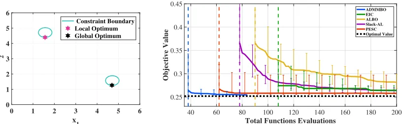
The left plot in Figure 1 shows the feasible region of (16) and its global and local optima, while the right figure shows the median of the objective value of the best feasible point, obtained by each method, among 100 runs as a function of total number of function evaluations. As the results demonstrate, ADMMBO outperforms EIC, ALBO, Slack-AL and PESC in terms of finding the global optimum at a lower budget. Moreover, ADMMBO is the first method to find a feasible point in all 100 runs, followed by PESC second and then the others. Only ADMMBO, ALBO, and Slack-AL have defined stopping criteria, and of those three only ADMBBO reaches its criterion and stops before the pre-set budget is exhausted. Figure 2 shows the best points obtained by ADMMBO, ALBO, and Slack-AL after 100 function evaluations, over 100 runs. Over all runs, ADMMBO has consistently found a feasible solution very close to the global optimum (black star in the left figure in Figure 1). However, the best points obtained by ALBO and Slack-AL are scattered throughout the entire feasible region and not necessarily close to the global optimum. Note that in a few runs, the best solutions found by these two methods are outside the feasible region, and thus are infeasible. We observe that ALBO and Slack-AL require a higher budget in order to converge to the global optimum of (16).
5.4. Test Problem with Multiple Constraints
0 1 2 3 4 5 6 x 1 0 1 2 3 4 5 6 x 2 Constraint Boundary Local Optimum Global Optimum
40 60 80 100 120 140 160 180 200
Total Functions Evaluations 0.25 0.3 0.35 0.4 0.45 Objective Value ADMMBO EIC ALBO Slack-AL PESC Optimal Value
Figure 1: Left: feasible region of (16) consists of two oval regions. The pink and black stars show, respectively, the local and global optimizer. Right: the curve of the median and 25/75 percentiles of the best objective value found by each method, among 100 runs that obtain a feasible solution, as a function of the total budget for function evaluation. We report the results of each method for a budget once all of its 100 runs obtain a feasible solution.
0 1 2 3 4 5 6
x 1 0 1 2 3 4 5 6 x2 Constraint Boundary ADMMBO Optimum
0 1 2 3 4 5 6
x 1 0 1 2 3 4 5 6 x 2 Constraint Boundary ALBO Optimum
0 1 2 3 4 5 6
x 1 0 1 2 3 4 5 6 x2 Constraint Boundary Slack-AL Optimum
Figure 2: Feasible region of (16) and the best solutions obtained by ADMMBO (left), ALBO (middle) and Slack-AL (right) after 100 function evaluations, over 100 runs. For each method, each point represents the final solution of that method over one run, after 100 total function evaluations.
constraints. More specifically, forB= [0,1]2, we consider the optimization problem min
x∈B x1+x2
s.t. 0.5 sin(2π(x21−2x2)) +x1+ 2x2+ 1.5≤0, −x21−x22+ 1.5≤0.
(17)
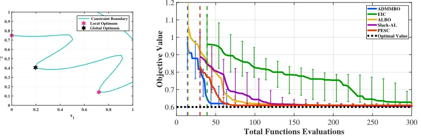
The left plot in Figure 3 shows the feasible region of (17) and its global and local optimizers, and the right plot shows the performance of different methods as a function of the number of function evaluation budget. The layout is the same as for the previous figure. Again, ADMMBO achieves the best performance in terms of converging to the global optimum at a lower budget, followed by PESC. We believe this is due to the fact that both ADMMBO and PESC can handle decoupled problems, including this example, via single function evaluations, while EIC, ALBO and Slack-AL enforce joint function evaluations at each step. Moreover, as the plot demonstrates, ADMMBO and ALBO are the first methods that arrive at a feasible point over 100 runs at a lower number of function evaluations.
0 0.2 0.4 0.6 0.8 1 x
1 0
0.1 0.2 0.3 0.4 0.5 0.6 0.7 0.8 0.9 1
x2
Constraint Boundary Local Optimum Global Optimum
0 50 100 150 200 250 300
Total Functions Evaluations
0.6 0.7 0.8 0.9 1 1.1 1.2
Objective Value
ADMMBO EIC ALBO Slack-AL PESC Optimal Value
Figure 3: Left: feasible region of the optimization problem (17). Right: performance of different methods as a function of the total budget for function evaluation.
0 0.2 0.4 0.6 0.8 1
x
1 0
0.2 0.4 0.6 0.8 1
x2
Constraint Boundary ADMMBO Optimum
0 0.2 0.4 0.6 0.8 1
x 1
0 0.2 0.4 0.6 0.8 1
x2
Constraint Boundary EIC Optimum
0 0.2 0.4 0.6 0.8 1
x 1 0
0.2 0.4 0.6 0.8 1
x2
Constraint Boundary PESC Optimum
Figure 4: The feasible region of (17) and the best solutions obtained by ADMMBO (left), EIC (middle) and PESC (right) after 50 function evaluations, over 100 runs. For each method, each point represents the final solution of that method over one run, after 50 total function evaluations.
its proposed solutions are scattered throughout the entire feasible region. According to the Figure 3, all methods, including EIC, ultimately converge to the global optimum. However, ADMMBO and PESC achieve this sooner and at a lower budget.
5.5. Test Problem in Higher Dimensions
0 20 40 60 80 100 120 140 160 180 200 Total Functions Evaluations
0 0.5 1 1.5 2 2.5 Objective Value ADMMBO EIC ALBO Slack-AL PESC Optimal Value
Figure 5: Performance of different algorithms solving (18) as a function of the total budget for function evaluation.
0 20 40 60 80 100 120
wall-clock time (minutes) 0 0.2 0.4 0.6 0.8 1 Validation Error ADMMBO PESC
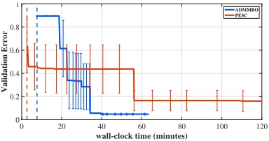
Figure 6: Comparison between ADMM and PESC for hyperparameter tuning for a neural network with short prediction time.
we consider the optimization problem
min x∈B 4 X i=1 xi
s.t. 1.1923 4
X
i=1
Eiexp −
4 X
j=1
Aji(xj−Pji)2
−1.1≤0
,
(18)
whereAji,Ei and Pji denote, respectively, the entries of
A=
10.00 0.05 3.00 17.00 3.00 10.00 3.50 8.00 17.00 17.00 1.70 0.05 3.50 0.10 10.00 10.00
, E=
1.0 1.2 3.0 3.2
, P =
0.131 0.232 0.234 0.404 0.169 0.413 0.145 0.882 0.556 0.830 0.352 0.873 0.012 0.373 0.288 0.574 .
As Figure 5 shows, ADMMBO and PESC compared to EIC, ALBO, and Slack-AL achieve lower value of the objective function after a smaller number of function evaluation. However, similar to other examples, ADMMBO arrives at a feasible point after fewer number of functions evaluations compared to PESC. As an interesting observation, in the budget range of [5,25], ADMMBO shows a flat curve, which we speculate is due to being at a local minima, however, finally ADMMBO escapes this local minimizer. Again, as this figure shows, an advantage of ADMMBO compared to existing work is its efficient stopping criterion that allows our algorithm to terminate before consuming the total budget, hence, avoiding unnecessary function evaluations.
5.6. Tuning a Fast Neural Network
to 0.045 second on NVIDIA Tesla K80 GPU. 2 Here, we focus on eleven hyperparam-eters: learning rate, decay rate, momentum parameter, two drop out probabilities for the input layer and the hidden layers as well as two regularization parameters for the weight decay, the weight maximum value, the number of hidden units in each of the 3 hidden layers, and the choice of activation function (RELU or sigmoid). We define
B= [0 1; 0 1; 0 1;−4 1; 0 100;−4 0;−3 0; 50 500; 50 500; 50 500; 0 1]. We build our network using Keras with TensorFlow backends (Chollet et al., 2015; Abadi et al., 2016). We com-pute the prediction time as the average time of 1000 predictions, over a batch size of 128 (Hern´andez-Lobato et al., 2015). Note that as mentioned in section 1, evaluating the pre-diction time may not require training the model and could be cheaply done using arbitrary weights.
We compare ADMMBO only with PESC, since as previously reported (Hern´ andez-Lobato et al., 2015, 2016) (and also consistent with our results on the synthetic experiments), PESC typically outperforms EIC and ALBO. Moreover, among state-of-the-art methods, ADMMBO and PESC are the only ones capable of handling decoupled problems, and thus are a good fit for this experiment. Note that since the computational cost of evaluating the validation error and the prediction time are significantly different, we show the results in terms of total wall-clock time rather than the total number of function evaluations.
As the results in Figure 6 show, PESC performed better at first. PESC found the first feasible set of hyperparameters slightly faster than ADMMBO, and also was able to find hyperparameters with lower validation error compared to the hyperparameters suggested by ADMMBO. However, around 18 minutes after initializing the algorithms, ADMMBO’s performance started to improve and outperformed PESC from minute 22 on. For exam-ple, at minute 40, ADMMBO found a desirable set of hyperparameters resulting in 0.05 validation error and less than 0.045 seconds prediction time. After the same time, PESC’s suggested hyperparameter result in a shorter prediction time less than 0.045 seconds, but their validation error was around 0.45. One interesting observation is that ADMMBO ter-minated after around one hour, satisfying its stopping criterion, avoiding extra expensive evaluations.
5.7. Sensitivity Analysis on M and ρ
In this section, we report on an evaluation of the sensitivity of ADMMBO to the hyper-parameters M and ρ. In the first set of experiments, we set the value ofM to 20 and ran ADMMBO for fifteen uniformly distributed initial values of ρ ∈ [0.0001,2], while keeping the rest of the hyperparameters as in 5.1. In Figure 7 we report on some selected cases, to avoid cluttering the figure. The figure illustrates that ADMMBO’s performance was not very sensitive to the initial value ofρ. In particular, for initialρ= 2, ADMMBO attained a feasible point over all 100 runs after no more than 27 function evaluations, while for other values ofρ, the same was achieved after roughly 15 evaluations. Even withρ= 2, at budget 15, 91 out of 100 runs had already found a feasible solution. The vertical dashed line in Figure 7 shows the budget at which the last run found a feasible solution.
0 50 100 150 Total Functions Evaluations
0.6 0.7 0.8 0.9 1
Objective Value
rho=0.001 rho=0.01 rho=0.1 rho=0.5 rho=1 rho=2 Optimal Value
Figure 7: Performance of ADMMBO solving (17) givenM = 20 and different values ofρ.
0 50 100 150
Total Functions Evaluations
0.6 0.7 0.8 0.9 1
Objective Value
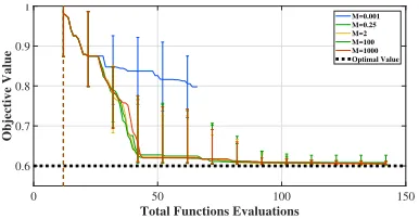
M=0.001 M=0.25 M=2 M=100 M=1000 Optimal Value
Figure 8: Performance of ADMMBO solving (17) givenρ= 0.1 and different values ofM.
In the second set of experiments, we set the value ofρto 0.1 and ran ADMMBO for ten uniformly distributed values ofM ∈[0.001,2] as well asM = 100,1000. As Figure 8 shows, again reporting on a subset of the values tested for clarity, the performance of ADMMBO did not depend strongly on the precise value of M as long as it was large enough. Note that in problem (17), the range off overBwas 2. Even forM <2, ADMMBO found good solutions, failing only when M was 4 order of magnitude smaller than the bound. Also, ADMMBO with different values of M found a feasible point over 100 runs at the same budget. Finally, given all different combinations of M andρ, ADMMBO always converged before spending the total iteration budget of 300.
6. DISCUSSION
In this paper, we address the problem of solving an optimization whose objective function and constraints are unknown and available to evaluate pointwise, but at high computational cost. We proposed a novel constrained Bayesian optimization algorithm, called ADMMBO, which merges ADMM, a powerful tool from numerical optimization, with Bayesian op-timization techniques. ADMMBO defines a set of unconstrained subproblems, over the modified objective function and over modified constraints, and iteratively solves them us-ing Bayesian optimization on each subproblem. Some key advantages of ADDMBO are its ability to start from an infeasible point, its ability to effectively handle decoupled problems, the ability to find closed-form acquisition functions, and its stopping criterion. We showed the effectiveness of ADMMBO through experiments on benchmark problems and the prob-lem of hyperparameter tuning for a fast neural network for digit recognition. ADMMBO consistently outperformed existing methods and obtained the feasible optimum with the fewest number of black-box evaluations. We speculate that the reason behind this rapid convergence is that ADMMBO typically first finds the unconstrained optimum of the prob-lem, and then looks for the closest point to that optimum which belongs to the feasible set, which turns out to be an effective search strategy.
principled ways of handling equality constraints is a topic for future investigation. Another extension of clear interest is to speed up ADMMBO through augmenting the problem with environmental variables which directly affect the duration of function evaluations (Klein et al., 2016). For example, in tuning the hyperparameters of a neural network, the size of the training set or the number of epochs can be regarded as such variable. Then, similar to Snoek et al. (2012), one can penalize ADMMBO’s acquisition functions with the inverse duration of function evaluations. We speculate that this may lead to finding a good solution for the unknown optimization problem as quickly as possible. A further extension concerns developing a comprehensive budget management strategy. This will be useful specifically in cases where we have partial knowledge about the unknown functions, in particular an estimate of the relative computational complexity of the objective and constraint functions. In this setting, we may be able to leverage such estimates to more efficiently distribute the budget. Another direction worth exploring is the flexibility within the ADMMBO frame-work to adopt different random process models (beyond independent GPs) and different acquisition functions (beyond EI). In particular using Predictive Entropy as acquisition function with approximations potentially similar to PESC-F would seem to be a promising approach to explore, given both the results in the literature and the relative success of PESC in our experiments. With any new acquisition function we would face the challenge of efficiently optimizing it. Acquisition functions are often multi-modal and complex, and it is an open question how best to carry out this particular optimization step.
Finally, we mention one current limitation of ADMMBO, which is the number of hyper-parameters. Good values will clearly speed up the optimization time of ADMMBO. In our experiments here, we followed the default initialization suggested in (Boyd et al., 2011; Hong and Luo, 2017) for the ADMM-related parameters and were able to obtain favorable results. However, for more complex problems, an adaptive initialization policy, potentially similar to ρ’s adaption rule based on primal and dual residuals suggested by Boyd et al. (2011), might make the algorithm less sensitive to the possibility of a poor parameter setting.
Acknowledgements
This project was supported by NIH grant R01CA199673 from NCI.
References
Mart´ın Abadi, Paul Barham, Jianmin Chen, Zhifeng Chen, Andy Davis, Jeffrey Dean, Matthieu Devin, Sanjay Ghemawat, Geoffrey Irving, Michael Isard, et al. Tensorflow: A system for large-scale machine learning. InOSDI, volume 16, pages 265–283, 2016.
Javad Azimi, Ali Jalali, and Xiaoli Fern. Hybrid batch bayesian optimization. arXiv preprint arXiv:1202.5597, 2012.
Pierre Baldi, Peter Sadowski, and Daniel Whiteson. Enhanced higgs boson to τ+τ- search with deep learning. Physical review letters, 114(11):111801, 2015.
James S Bergstra, R´emi Bardenet, Yoshua Bengio, and Bal´azs K´egl. Algorithms for hyper-parameter optimization. InAdvances in neural information processing systems, pages 2546–2554, 2011.
L´eon Bottou. Large-scale machine learning with stochastic gradient descent. In Proceedings of COMPSTAT’2010, pages 177–186. Springer, 2010.
Stephen Boyd, Neal Parikh, Eric Chu, Borja Peleato, and Jonathan Eckstein. Distributed optimiza-tion and statistical learning via the alternating direcoptimiza-tion method of multipliers. Foundations and TrendsR in Machine Learning, 3(1):1–122, 2011.
Eric Brochu, Tyson Brochu, and Nando de Freitas. A bayesian interactive optimization approach to procedural animation design. In Proceedings of the 2010 ACM SIGGRAPH/Eurographics Symposium on Computer Animation, pages 103–112. Eurographics Association, 2010a.
Eric Brochu, Vlad M Cora, and Nando De Freitas. A tutorial on bayesian optimization of expensive cost functions, with application to active user modeling and hierarchical reinforcement learning.
arXiv preprint arXiv:1012.2599, 2010b.
Fran¸cois Chollet et al. Keras, 2015.
Dennis D Cox and Susan John. A statistical method for global optimization. InSystems, Man and Cybernetics, 1992., IEEE International Conference on, pages 1241–1246. IEEE, 1992.
Daniel E Finkel. Direct optimization algorithm user guide. Center for Research in Scientific Com-putation, North Carolina State University, 2, 2003.
Jacob R Gardner, Matt J Kusner, Zhixiang Eddie Xu, Kilian Q Weinberger, and John P Cunning-ham. Bayesian optimization with inequality constraints. InICML, pages 937–945, 2014.
Michael A Gelbart, Jasper Snoek, and Ryan P Adams. Bayesian optimization with unknown con-straints. arXiv preprint arXiv:1403.5607, 2014.
Michael Adam Gelbart. Constrained Bayesian Optimization and Applications. PhD thesis, 2015.
Robert B Gramacy, Genetha A Gray, S´ebastien Le Digabel, Herbert KH Lee, Pritam Ranjan, Garth Wells, and Stefan M Wild. Modeling an augmented lagrangian for blackbox constrained optimization. Technometrics, 58(1):1–11, 2016.
Jos´e Miguel Hern´andez-Lobato, Matthew W Hoffman, and Zoubin Ghahramani. Predictive entropy search for efficient global optimization of black-box functions. InAdvances in neural information processing systems, pages 918–926, 2014.
Jos´e Miguel Hern´andez-Lobato, Michael Gelbart, Matthew Hoffman, Ryan Adams, and Zoubin Ghahramani. Predictive entropy search for bayesian optimization with unknown constraints. In
International Conference on Machine Learning, pages 1699–1707, 2015.
Jos´e Miguel Hern´andez-Lobato, Michael A Gelbart, Ryan P Adams, Matthew W Hoffman, and Zoubin Ghahramani. A general framework for constrained bayesian optimization using information-based search. 2016.
Matthew Hoffman, Bobak Shahriari, and Nando Freitas. On correlation and budget constraints in model-based bandit optimization with application to automatic machine learning. In Artificial Intelligence and Statistics, pages 365–374, 2014.
Mingyi Hong, Zhi-Quan Luo, and Meisam Razaviyayn. Convergence analysis of alternating direction method of multipliers for a family of nonconvex problems. SIAM Journal on Optimization, 26(1): 337–364, 2016.
Neil Houlsby, Ferenc Huszar, Zoubin Ghahramani, and Jose M Hern´andez-Lobato. Collaborative gaussian processes for preference learning. InAdvances in Neural Information Processing Systems, pages 2096–2104, 2012.
Frank Hutter, Holger H Hoos, and Kevin Leyton-Brown. Sequential model-based optimization for general algorithm configuration. In International Conference on Learning and Intelligent Optimization, pages 507–523. Springer, 2011.
Donald R Jones. A taxonomy of global optimization methods based on response surfaces. Journal of global optimization, 21(4):345–383, 2001.
Donald R Jones, Matthias Schonlau, and William J Welch. Efficient global optimization of expensive black-box functions. Journal of Global optimization, 13(4):455–492, 1998.
Aaron Klein, Stefan Falkner, Simon Bartels, Philipp Hennig, and Frank Hutter. Fast bayesian opti-mization of machine learning hyperparameters on large datasets.arXiv preprint arXiv:1605.07079, 2016.
Harold J Kushner. A new method of locating the maximum point of an arbitrary multipeak curve in the presence of noise. Journal of Basic Engineering, 86(1):97–106, 1964.
Yann LeCun. The mnist database of handwritten digits. http://yann. lecun. com/exdb/mnist/, 1998.
Yann LeCun, Yoshua Bengio, and Geoffrey Hinton. Deep learning. nature, 521(7553):436, 2015.
Daniel James Lizotte. Practical bayesian optimization. University of Alberta, 2008.
Ruben Martinez-Cantin, Nando de Freitas, Arnaud Doucet, and Jos´e A Castellanos. Active policy learning for robot planning and exploration under uncertainty. InRobotics: Science and Systems, volume 3, pages 334–341, 2007.
Thomas Peter Minka. A family of algorithms for approximate Bayesian inference. PhD thesis, Massachusetts Institute of Technology, 2001.
J Moˇckus. On bayesian methods for seeking the extremum. In Optimization Techniques IFIP Technical Conference, pages 400–404. Springer, 1975.
Joao FC Mota, Joao MF Xavier, Pedro MQ Aguiar, and Markus Puschel. D-admm: A communication-efficient distributed algorithm for separable optimization. IEEE Transactions on Signal Processing, 61(10):2718–2723, 2013.
Jorge Nocedal and Stephen J. Wright. Numerical Optimization. Springer, New York, NY, USA, second edition, 2006.
Neal Parikh, Stephen Boyd, et al. Proximal algorithms. Foundations and TrendsR in Optimization,
1(3):127–239, 2014.
Victor Picheny. A stepwise uncertainty reduction approach to constrained global optimization. In
Victor Picheny, David Ginsbourger, Yann Richet, and Gregory Caplin. Quantile-based optimization of noisy computer experiments with tunable precision. Technometrics, 55(1):2–13, 2013.
Victor Picheny, Robert B Gramacy, Stefan Wild, and Sebastien Le Digabel. Bayesian optimization under mixed constraints with a slack-variable augmented lagrangian. In Advances in Neural Information Processing Systems, pages 1435–1443, 2016.
Carl Edward Rasmussen and Christopher KI Williams. Gaussian processes for machine learning, volume 1. MIT press Cambridge, 2006.
Matthias Schonlau, William J Welch, and Donald R Jones. Global versus local search in constrained optimization of computer models. Lecture Notes-Monograph Series, pages 11–25, 1998.
Steven L Scott. A modern bayesian look at the multi-armed bandit. Applied Stochastic Models in Business and Industry, 26(6):639–658, 2010.
Bobak Shahriari, Kevin Swersky, Ziyu Wang, Ryan P Adams, and Nando de Freitas. Taking the human out of the loop: A review of bayesian optimization. Proceedings of the IEEE, 104(1): 148–175, 2016.
Jasper Snoek. Bayesian optimization and semiparametric models with applications to assistive tech-nology. PhD thesis, Citeseer, 2013.
Jasper Snoek, Hugo Larochelle, and Ryan P Adams. Practical bayesian optimization of machine learning algorithms. In Advances in neural information processing systems, pages 2951–2959, 2012.
Kevin Swersky, Jasper Snoek, and Ryan P Adams. Multi-task bayesian optimization. InAdvances in neural information processing systems, pages 2004–2012, 2013.
Robert Tibshirani. Regression shrinkage and selection via the lasso.Journal of the Royal Statistical Society. Series B (Methodological), pages 267–288, 1996.
Aimo Torn and Antanas Zilinskas. Global optimization. Springer-Verlag New York, Inc., 1989.
Yu Wang, Wotao Yin, and Jinshan Zeng. Global convergence of admm in nonconvex nonsmooth optimization. Journal of Scientific Computing, pages 1–35, 2015.
Jian Wu, Matthias Poloczek, Andrew G Wilson, and Peter Frazier. Bayesian optimization with gradients. InAdvances in Neural Information Processing Systems, pages 5273–5284, 2017.