COEVOLVE: A Joint Point Process Model for Information
Diffusion and Network Evolution
∗3Mehrdad Farajtabar [email protected]
College of Computing
Georgia Institute of Technology Atlanta, GA 30332, USA
Yichen Wang [email protected]
College of Computing
Georgia Institute of Technology Atlanta, GA 30332, USA
Manuel Gomez-Rodriguez [email protected]
MPI for Software Systems
Paul-Ehrlich-Strasse, 67663 Kaiserslautern Germany
Shuang Li [email protected]
H. Milton Stewart School of Industrial and Systems Engineering Georgia Institute of Technology
Atlanta, GA 30332, USA
Hongyuan Zha [email protected]
College of Computing
Georgia Institute of Technology Atlanta, GA 30332, USA
Le Song [email protected]
College of Computing
Georgia Institute of Technology Atlanta, GA 30332, USA
Editor:Edo Airoldi
Abstract
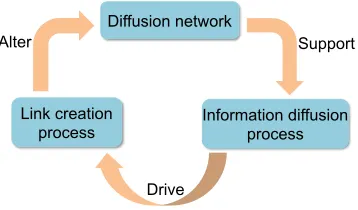
Information diffusion in online social networks is affected by the underlying network topology, but it also has the power to change it. Online users are constantly creating new links when exposed to new information sources, and in turn these links are alternating the way information spreads. However, these two highly intertwined stochastic processes, information diffusion and network evolution, have been predominantly studiedseparately, ignoring their co-evolutionary dynamics.
We propose a temporal point process model, Coevolve, for such joint dynamics, allowing the intensity of one process to be modulated by that of the other. This model allows us to efficiently simulate interleaved diffusion and network events, and generate
. ∗Preliminary version of this work appeared in (Farajtabar et al., 2015b).
. 3 Implementation codes are available athttps://github.com/farajtabar/Coevolution
c
traces obeying common diffusion and network patterns observed in real-world networks such as Twitter. Furthermore, we also develop a convex optimization framework to learn the parameters of the model from historical diffusion and network evolution traces. We experimented with both synthetic data and data gathered from Twitter, and show that our model provides a good fit to the data as well as more accurate predictions than alternatives.
Keywords: social networks, information diffusion, network structure, co-evolutionary dynamics, point processes, Hawkes process, survival analysis
1. Introduction
Online social networks, such as Twitter or Weibo, have become large information net-works where people share, discuss and search for information of personal interest as well as
breaking news (Kwak et al., 2010). In this context, users often forward to their followers
information they are exposed to via theirfollowees, triggering the emergence of information
cascades that travel through the network (Cheng et al., 2014), and constantly create new links to information sources, triggering changes in the network itself over time. Importantly, recent empirical studies with Twitter data have shown that both information diffusion and network evolution are coupled and network changes are often triggered by information dif-fusion (Antoniades and Dovrolis, 2015; Weng et al., 2013; Myers and Leskovec, 2014).
While there have been many recent works on modeling information diffusion (Gomez-Rodriguez et al., 2010; Du et al., 2013; Cheng et al., 2014; Farajtabar et al., 2015a) and network evolution (Chakrabarti et al., 2004; Leskovec et al., 2008, 2010), most of them treat these two stochastic processes independently and separately, ignoring the influence one may have on the other over time. More notably, Weng et al. (2013) were the first to show experimental evidence that information diffusion influences network evolution in microblogging sites both at system-wide and individual levels. In particular, they studied
Yahoo! Meme, a social micro-blogging site similar to Twitter, which was active between 2009 and 2012, and showed that information diffusion causes about 24 % of the new links, and that the likelihood of a new link from a user to another increases with the number of posts by the second user seen by the first one. Also, Antoniades and Dovrolis (2015) studied the temporal characteristics of retweet-driven connections within the Twitter network and realized that the number of retweets is an important factor to infer such connections. They showed that links created due to information diffusion account for 42 % of new links, and are rather infrequent, compared to tweets and retweets, but they are responsible for a large percentage of the new links in Twitter.
However, there are a few limitations in the above-mentioned studies. First, they only characterize the effect that information diffusion has on the network dynamics, or the vice versa, but not the bidirectional influence. Second, previous studies are mostly empirical and only make binary predictions on link creation events without precise timing. For example, the work of (Weng et al., 2013; Antoniades and Dovrolis, 2015) predict whether a new link will be created based on the number of retweets; and, Myers and Leskovec (2014) predict whether a burst of new links will occur based on the number of retweets and users’ similarity. Thus, to better understand information diffusion and network evolution, there is an urgent need for joint probabilistic models of the two processes, which are largely inexistent to date.
In this paper, we propose a probabilistic generative model, Coevolve, for the joint
Diffusion network
Information diffusion process
Drive Link creation
process
Support Alter
Figure 1: Illustration of how information diffusion and network structure processes interact
model is able to learn parameters from real world data, and predict the precise timing of both diffusion and new link events. The proposed model is based on the framework of temporal point processes, which explicitly characterizes the continuous time interval between events, and it consists of two interwoven and interdependent components, as shown in Figure 1:
I. Information diffusion process. We design an “identity revealing” multivariate Hawkes process (Farajtabar et al., 2014) to capture the mutual excitation behavior of retweeting events, where the intensity of such events in a user is boosted by previous events from her time-varying set of followees. Although Hawkes processes have been used for information diffusion before (Farajtabar et al., 2016; Blundell et al., 2012; Iwata et al., 2013; Zhou et al., 2013a; Farajtabar et al., 2014; Linderman and Adams, 2014; Valera and Gomez-Rodriguez, 2015), the key innovation of our approach is to explicitly model the excitation due to a particular source node, hence revealing the identity of the source. Such design reflects the reality that information sources are explicitly acknowledged, and it also allows a particular information source to acquire new links in a rate according to her “informativeness”.
II. Network evolution process. We model link creation as an “information driven” survival process, and couple the intensity of this process with retweeting events. Al-though survival processes have been used for link creation before (Hunter et al., 2011; Vu et al., 2011), the key innovation in our model is to incorporate retweeting events as the driving force for such processes. Since our model has captured the source identity of each retweeting event, new links will be targeted toward information sources, with an intensity proportional to their degree of excitation and each source’s influence.
Our model is designed in such a way that it allows the two processes, information diffusion and network evolution, unfold simultaneously in the same time scale and exercise bidirectional influence on each other, allowing sophisticated coevolutionary dynamics to be generated, as illustrated in Figure 2.
Importantly, the flexibility of our model does not prevent us from efficiently simulating diffusion and link events from the model and learning its parameters from real world data:
• Efficient simulation. We design a scalable sampling procedure that exploits the
sparsity of the generated networks. Its complexity is O(ndlogm), where n is the
number of events,mis the number of users anddis the maximum number of followees
Christine
Sophie
David
Jacob
Bob 1pm, D: Cool paper
1:10pm, @D: Indeed
1:30pm, @S @D: Very useful
2:03pm, @D: I want that car 1:20pm @C @S @D:
Really? Will check
2pm, D: Nice car
1:35pm @B @S @D: Indeed brilliant
1:45pm
D S
means S follows D
1:15pm, @S @D: Classic
Figure 2: Illustration of information diffusion and network structure co-evolution.
Information diffusion → network structure: David’s tweet at 1:00 pm about a
paper is retweeted by Sophie and Christine respectively at 1:10 pm and 1:15 pm to reach out to Jacob. Jacob retweets about this paper at 1:20 pm and 1:35 pm and then finds David a good source of information and decides to follow him directly at 1:45 pm.
Information diffusion→ network structure: As a result new path of information
from David to Jacob (and his downstream followers) is created. Consequently, a subsequent tweet by David about a car at 2:00 pm directly reaches out to Jacob without need to Sophie and Christine retweet.
• Convex parameters learning. We show that the model parameters that maximize the joint likelihood of observed diffusion and link creation events can be efficiently found via convex optimization.
Then, we experiment with our model and show that it can produce coevolutionary dynamics of information diffusion and network evolution, and generate retweet and link events that
obey common information diffusion patterns (e.g., cascade structure, size and depth), static
network patterns (e.g., node degree) and temporal network patterns (e.g., shrinking
diam-eter) described in related literature (Leskovec et al., 2005, 2010; Goel et al., 2012). Finally, we show that, by modeling the coevolutionary dynamics, our model provides significantly more accurate link and diffusion event predictions than alternatives in large scale Twitter data set (Antoniades and Dovrolis, 2015).
The remainder of this article is organized as follows. We first proceed by building
𝑡 𝑓∗(𝑡)
𝑆∗(𝑡)
Pr. event survives after 𝑡 (survival function)
𝐹∗(𝑡)
Pr. event occurs before 𝑡 (cdf)
𝑡 + 𝑑𝑡 𝑡 𝑓∗𝑡 𝑑𝑡
Pr. event occurs between [𝑡, 𝑡 + d𝑡]
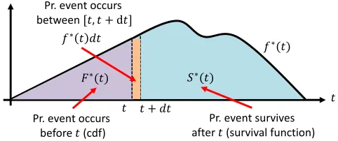
Figure 3: Illustration of three inter-related quantities in point processes framework: con-ditional density function, concon-ditional cumulative density function, and survival function.
In Sections 6, 7, and 8 we perform empirical investigation of the properties of the model, we evaluate the accuracy of the parameter estimation in synthetic data, and we evaluate the performance of the proposed model in the real-world data set, respectively. Section 9 reviews the related work, and finally, the paper is concluded in Section 10. Proofs, more detailed contents and experimental results, and some extensions are left to the appendices.
2. Background on Temporal Point Processes
A temporal point process is a random process whose realization consists of a list of discrete
events localized in time, {ti} with ti ∈ R+ and i ∈ Z+. Many different types of data
produced in online social networks can be represented as temporal point processes, such as the times of retweets and link creations. A temporal point process can be equivalently
represented as a counting process,N(t), which records the number of events before time t.
Let the history H(t) be the list of times of events {t1, t2, . . . , tn} up to but not including
timet. Then, the number of observed events in a small time window [t, t+dt) of lengthdt
is
dN(t) = X
ti∈H(t)
δ(t−ti)dt, (1)
and hence N(t) =Rt
0dN(s), where δ(t) is a Dirac delta function. More generally, given a
functionf(t), we can define the convolution with respect todN(t) as
f(t) ? dN(t) := Z t
0
f(t−τ)dN(τ) =X
ti∈H(t)
f(t−ti). (2)
The point process representation of temporal data is fundamentally different from the dis-crete time representation typically used in social network analysis. It directly models the time interval between events as random variables, avoids the need to pick a time window to aggregate events, and allows temporal events to be modeled in a fine grained fashion. Moreover, it has a remarkably rich theoretical support (Aalen et al., 2008).
An important way to characterize temporal point processes is via the conditional in-tensity function—a stochastic model for the time of the next event given all the times of
a) Poisson process
𝜆∗ 𝑡 = 𝜇
𝑡
b) Hawkes process
𝜆∗ 𝑡 = 𝜇 + 𝛼
𝑡𝑖<𝑡
exp −|𝑡 − 𝑡𝑖| = 𝜇 + 𝛼 𝜅𝜔(𝑡)⋆ 𝑑𝑁(𝑡)
𝑡
c) Survival process
𝜆∗ 𝑡 = 1 − 𝑁 𝑡 𝑔(𝑡)
𝑡
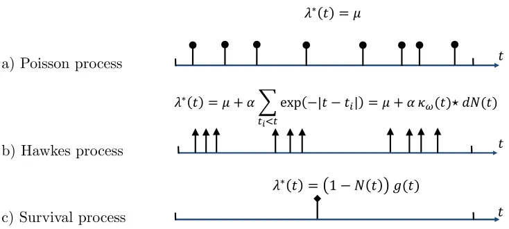
Figure 4: Three types of point processes with a typical realization
the conditional probability of observing an event in a small window [t, t+dt) given the
historyH(t), i.e.,
λ∗(t)dt:=P{event in [t, t+dt)|H(t)}=E[dN(t)|H(t)], (3)
where one typically assumes that only one event can happen in a small window of size dt
and thusdN(t)∈ {0,1}. Then, given the observation until time tand a timet0 >t, we can
also characterize the conditional probability that no event happens until t0 as
S∗(t0) = exp − Z t0
t
λ∗(τ)dτ
!
, (4)
the (conditional) probability density function that an event occurs at time t0 as
f∗(t0) =λ∗(t0)S∗(t0), (5)
and the (conditional) cumulative density function, which accounts for the probability that
an event happens before timet0:
F∗(t0) = 1−S∗(t0) = Z t0
t
f∗(τ)dτ. (6)
Figure 3 illustrates these quantities. Moreover, we can express the log-likelihood of a list of events {t1, t2, . . . , tn}in an observation window [0, T) as
L=
n
X
i=1
logλ∗(ti)−
Z T
0
λ∗(τ)dτ, T >tn. (7)
This simple log-likelihood will later enable us to learn the parameters of our model from
observed data. Finally, the functional form of the intensityλ∗(t) is often designed to capture
the phenomena of interests. Some useful functional forms we will use are (Aalen et al., 2008):
(i) Poisson process. The intensity is assumed to be independent of the history H(t),
but it can be a nonnegative time-varying function,i.e.,
(ii) Hawkes process. The intensity is history dependent and models a mutual excitation
between events,i.e.,
λ∗(t) =µ+ακω(t)? dN(t) =µ+α
X
ti∈H(t)
κω(t−ti), (9)
where,
κω(t) := exp(−ωt)I[t>0] (10)
is an exponential triggering kernel and µ > 0 is a baseline intensity independent of
the history. Here, the occurrence of each historical event increases the intensity by a
certain amount determined by the kernel and the weightα >0, making the intensity
history dependent and a stochastic process by itself. In our work, we focus on the exponential kernel, however, other functional forms, such as log-logistic function, are possible, and the general properties of our model do not depend on this particular choice.
(iii) Survival process. There is only one event for an instantiation of the process,i.e.,
λ∗(t) = (1−N(t))g(t), (11)
where g(t) > 0 and the term (1−N(t)) makes sure λ∗(t) is 0 if an event already
happened beforet.
Figure 4 illustrates these processes. Interested reader should refer to Aalen et al. (2008) for more details on the framework of temporal point processes.
Point process models have been applied to many tasks in networks such as fake news mitigation (Farajtabar et al., 2017), recommendation systems (Hosseini et al., 2017), outlier detection (Li et al., 2017), activity shaping in social networks (Farajtabar et al., 2014), veri-fying crowd-generated data (Tabibian et al., 2017), sequence modeling using deep recurrent neural networks (Xiao et al., 2017), and campaigning in networks (Farajtabar et al., 2016).
3. Generative Model of Information Diffusion and Network Evolution
In this section, we use the above background on temporal point processes to formulate
Coevolve, our probabilistic model for the joint dynamics of information diffusion and
network evolution.
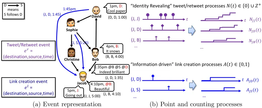
3.1 Event Representation
We model the generation of two types of events: tweet/retweet events,er, and link creation
events, el. Instead of just the time t, we record each event as a triplet, as illustrated in
Figure 5(a):
er or el := ( u
↑
destination
,
source
↓
s, t
↑
time
). (12)
For retweet event, the triplet means that the destination node u retweets at time
t a tweet originally posted by source node s. Recording the source node s reflects the
real world scenario that information sources are explicitly acknowledged. Note that the
D S means S follows D
1pm, D:
Cool paper (D, D, 1:00)
1:35pm @B @S @D:
Indeed brilliant (J, D, 1:35)
4:10pm, @B:
Beautiful (J, B, 4:10)
4pm, B:
It snows (B, B, 4:00) (J, D, 1:45)
5pm, J:
Going out (J, J, 5:00) (J, S, 5:25) 1:45pm
Christine Sophie
David
Jacob Bob
Link creation event 𝑒𝑙 =
(destination,source,time) Tweet/Retweet event
𝑒𝑟 =
(destination,source,time)
“Identity Revealing” tweet/retweet processes 𝑁 𝑡 ∈ 0 ∪ 𝑍+
“Information driven” link creation processes 𝐴 𝑡 ∈ {0,1}
𝑡 (J, D)
(J, S)
… …
𝑡 𝐴𝐽𝐷(𝑡)
𝐴𝐽𝑆(𝑡) 𝑡
(J, J)
(J, D)
(J, B) …
𝑡 𝑁𝐽𝐽(𝑡)
𝑁𝐽𝐷(𝑡)
𝑁𝐽𝐵(𝑡)
…
(a) Event representation (b) Point and counting processes
Figure 5: Events of point processes and their associated counting processes for link creation and information diffusion; (a) Trace of events generated by a tweet from David followed by new links Jacob creates to follow David and Sophie; (b) The associated points in time and the counting process realizations.
to s. This event can happen when u is retweeting a message by another node u0 where
the original information source s is acknowledged. Node u will pass on the same source
acknowledgement to its followers (e.g., “I agree @a @b @c @s”). Original tweets posted by
node u are allowed in this notation. In this case, the event will simply be er = (u, u, t).
Given a list of retweet events up to but not including timet, the history Hr
us(t) of retweets
by u due to sourcesis
Hrus(t) ={eri = (ui, si, ti)|ui =u and si=s}. (13)
The entire history of retweet events is denoted as
Hr(t) :=∪
u,s∈[m]Hrus(t). (14) For link creation event, the triplet means that destination node u creates at time
t a link to source node s, i.e., from time t on, node u starts following node s. To ease
the exposition, we restrict ourselves to the case where links cannot be deleted and thus each (directed) link is created only once. However, our model can be easily augmented to consider multiple link creations and deletions per node pair, as discussed in Section E. We
denote the link creation history asHl(t).
3.2 Joint Model with Two Interwoven Components
Given m users, we use two sets of counting processes to record the generated events, one
for information diffusion and another for network evolution. More specifically,
I. Retweet events are recorded using a matrix N(t) of size m×m for each fixed time
point t. The (u, s)-th entry in the matrix, Nus(t)∈ {0} ∪Z+, counts the number of
retweets of u due to source s up to time t. These counting processes are “identity
matrixN(t) is typically less sparse thanA(t), sinceNus(t) can be nonzero even when
nodeu does not directly follow s. We also letdN(t) := ( dNus(t) )u,s∈[m].
II. Link events are recorded using an adjacency matrixA(t) of sizem×m for each fixed
time pointt. The (u, s)-th entry in the matrix,Aus(t)∈ {0,1}, indicates whetheruis
directly followings. Therefore, Aus(t) = 1 means the directed link has been created
beforet. For simplicity of exposition, we do not allow self-links. The matrix A(t) is
typically sparse, but the number of nonzero entries can change over time. We also definedA(t) := ( dAus(t) )u,s∈[m].
Then, the interwoven information diffusion and network evolution processes can be charac-terized using their respective intensities
E[dN(t)| Hr(t)∪ Hl(t)] =Γ∗(t)dt (15)
E[dA(t)| Hr(t)∪ Hl(t)] =Λ∗(t)dt, (16)
where,
Γ∗(t) = (γus∗ (t) )u,s∈[m] (17)
Λ∗(t) = (λ∗us(t) )u,s∈[m]. (18)
The sign∗ means that the intensity matrices will depend on the joint history,Hr(t)∪ Hl(t),
and hence their evolution will be coupled. By this coupling, we make: (i) the counting processes for link creation to be “information driven” and (ii) the evolution of the linking structure to change the information diffusion process. In the next two sections, we will specify the details of these two intensity matrices.
3.3 Information Diffusion Process
We model the intensity,Γ∗(t), for retweeting events using multivariate Hawkes process:
γ∗us(t) =I[u=s]ηu+I[u6=s]βs
X
v∈Fu(t)κω1(t)?(Auv(t) dNvs(t)), (19)
where I[·] is the indicator function and Fu(t) := {v∈[m] :Auv(t) = 1} is the current set
of followees of u. The term ηu > 0 is the intensity of original tweets by a user u on
his own initiative, becoming the source of a cascade, and the term βsPv∈Fu(t)κω1(t) ?
(Auv(t)dNvs(t)) models the propagation of peer influence over the network, where the
triggering kernel κω1(t) models the decay of peer influence over time.
Note that the retweeting intensity matrix Γ∗(t) is by itself a stochastic process that
depends on the time-varying network topology, the non-zero entries inA(t), whose growth is
controlled by the network evolution process in Section 3.4. Hence the model design captures
the influence of the network topology and each source’s influence, βs, on the information
diffusion process. More specifically, to computeγus∗ (t), one first finds the current setFu(t)
of followees ofu, and then aggregates the retweets of these followees that are due to sources.
Note that these followees may or may notdirectly follow sources. Then, the more frequently
nodeuis exposed to retweets of tweets originated from sourcesvia her followees, the more
likely she will also retweet a tweet originated from source s. Once node u retweets due to
source s, the correspondingNus(t) will be incremented, and this in turn will increase the
likelihood of triggering retweets due to source samong the followers of u. Thus, the source
1 − 𝐴𝐽𝐷𝑡 ⋅ 𝜇𝐽+ 𝛼𝐽exp − 𝑡 ⋆ 𝑑𝑁𝐽𝐶 𝑡 + 𝑑𝑁𝐽𝐵𝑡
𝜆𝐽𝐷∗ 𝑡 =
Check whether
the link already there
Retweet through B Hawkes process Initiative coming from
neighbors Survival Process
High intensity when no link and retweet often
Poisson process User 𝐽’s
own initiative
Retweet through C
𝐸[𝑑𝐴𝐽𝐷𝑡 ] = 𝜆𝐽𝐷∗ 𝜏 𝑑𝜏
D S
means S follows D
Christine Sophie
David
Jacob Bob
1:45pm
𝑁𝐵𝐷𝑡
𝑁𝐶𝐷𝑡
𝑁𝐷𝐷 𝑡
𝐸[𝑑𝑁𝐷𝐷𝑡 ] = 𝛾𝐷𝐷∗ 𝜏 𝑑𝜏
𝛽𝐷exp − 𝑡 ⋆ 𝐴𝐽𝐵𝑡 𝑑𝑁𝐵𝐷𝑡 + 𝐴𝐽𝐶𝑡 𝑑𝑁𝐶𝐷𝑡 𝛾𝐽𝐷∗ 𝑡 =
Exposure due to 𝐶
Exposure due to 𝐵
Aggregate exposure from all followees Hawkes process High intensity with more exposure
𝐸[𝑑𝑁𝐽𝐷𝑡 ] = 𝛾𝐽𝐷∗ 𝜏 𝑑𝜏
Poisson process User 𝐷’s own initiative
𝛾𝐷𝐷∗ 𝑡 = 𝜂𝐷
(a) Link creation process (b) Social network (c) Information diffusion process
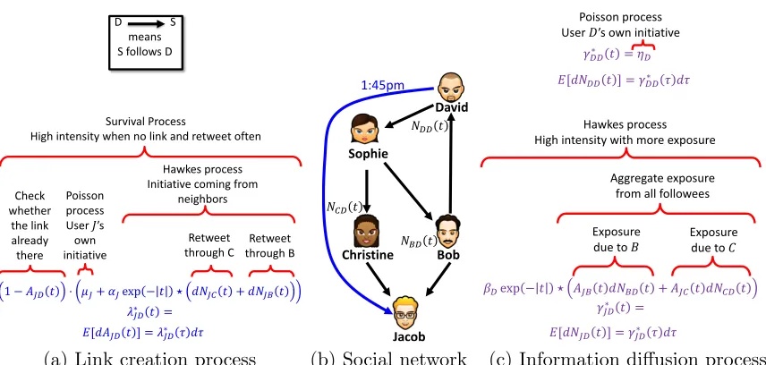
Figure 6: Our hypothetical social network where the information diffusion paths make Ja-cob follow David: (a) The breakdown of conditional intensity function for the link
creation process of Jacob following DavidAJ D(t); (b) The information paths
be-tween Jacob and David; (c) The information diffusion processes for David tweeting
on his own initiativeNDD(t) and Jacob retweeting posts originated from David
NJ D(t).
propagates through the network even to those nodes that do not directly follow her. Finally, this information diffusion model allows a node to repeatedly generate events in a cascade, and is very different from the independent cascade or linear threshold models (Kempe et al., 2003) which allow at most one event per node per cascade.
3.4 Network Evolution Process
In our model, each user is exposed to information through a time-varying set of neighbors. By doing so, information diffusion affects network evolution, increasing the practical appli-cation of our model to real-world network data sets. The particular definition of exposure
(e.g., a retweet’s neighbor) depends on the type of historical information that is available.
Remarkably, the flexibility of our model allows for different types of diffusion events, which we can broadly classify into two categories.
In the first category, events corresponds to the times when an information cascade hits a person, for example, through a retweet from one of her neighbors, but she does not explicitly
like or forward the associated post. Here, we model the intensity, Λ∗(t), for link creation
using a combination of survival and Hawkes process:
λ∗us(t) = (1−Aus(t))
µu+αu
X
v∈Fu(t)
κω2(t)? dNvs(t)
where the term 1−Aus(t) effectively ensures a link is created only once, and after that, the
corresponding intensity is set to zero. The termµu >0 denotes a baseline intensity, which
models when a nodeudecides to follow a sourcesspontaneously at her own initiative. The
termαuκω2(t)? dNvs(t) corresponds to the retweets by nodev (a followee of nodeu) which
are originated from sources. The triggering kernelκω2(t) models the decay of interests over
time.
In the second category, the person decides to explicitly like or forward the associated post and influencing events correspond to the times when she does so. In this case, we model the intensity, Λ∗(t), for link creation as:
λ∗us(t) = (1−Aus(t))(µu+αuκω2(t)? dNus(t)), (21)
where the terms 1−Aus(t), µu > 0, and the decaying kernel κω2(t) play the same role
as the corresponding ones in Equation (20). The term αuκω2(t)? dNus(t) corresponds to
the retweets of node u due to tweets originally published by source s. The higher the
corresponding retweet intensity, the more likely u will find information by source s useful
and will create a direct link tos.
In both cases, the link creation intensity Λ∗(t) is also a stochastic process by itself,
which depends on the retweet events, be it the retweets by the neighbors of node u or the
retweets by nodeu herself, respectively. Therefore, it captures the influence of retweets on
the link creation, and closes the loop of mutual influence between information diffusion and network topology. Figure 6 illustrates these two interdependent intensities.
Intuitively, in the latter category, information diffusion events are more prone to trigger new connections, because, they involve the target and source nodes in an explicit interaction, however, they are also less frequent. Therefore, it is mostly suitable to large event data sets, as the ones we generate in our synthetic experiments. In contrast, in the former category, information diffusion events are less likely to inspire new links but found in abundance. Therefore, it is more suitable for smaller data sets, as the ones we use in our real-world experiments. Consequently, in our synthetic experiments we used the latter and in our real-world experiments, we used the former.
More generally, the choice of exposure event should be made based on the type and amount of available historical information. Note that, these are two realizations, among
the many others, of the link formation process in the Coevolve framework. Many other
extensions can be found in appendix E. In practice, these different forms can be utilized depending on the conditions and constraints of the networks and the data in hand. More importantly, in this section, we make one example on how to tailor the model to fit the application best.
Finally, note that creating a link is more than just adding a path or allowing informa-tion sources to take shortcuts during diffusion. The network evoluinforma-tion makes fundamental changes to the diffusion dynamics and stationary distribution of the diffusion process in
Section 3.3. As shown in Farajtabar et al. (2014), given a fixed network structure A,
the expected retweet intensity µs(t) at time t due to source s will depend of the network
structure in a nonlinear fashion,i.e.,
µs(t) :=E[Γ∗·s(t)] = (e(A−ω1I)t+ω1(A−ω1I)−1(e(A−ω1I)t−I))ηs, (22)
where ηs ∈Rm has a single nonzero entry with value ηs and e(A−ω1I)t is the matrix
t
λU
*(t') λ2
*(t')
λ1 *
(t')
+
+
+
=
t' λ2
* (τ) λ1
*( τ)
λU
*(
τ)
λsum* (
τ)
τ
τ
τ
τ
t τmin
τ2
τ1
τU τ
τ
τ
τ λ2
*( τ) λ1
*(
τ)
λU*( τ)
(a) Ogata’s algorithm (b) Proposed algorithm
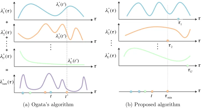
Figure 7: Ogata’s algorithm vs our simulation algorithm in simulating U interdependent
point processes characterized by intensity functionsλ1(t), . . . , λU(t); (a)
Illustrat-ing Ogata’s algorithm, which first takes a sample from the process with intensity equal to sum of individual intensities and then assigns it to the proper dimension proportionally to its contribution to the sum of intensities; (b) Illustrating our proposed algorithm, which first draws a sample from each dimension indepen-dently and then takes the minimum time among them.
related to the network structure. Thus, given two network structures A(t) and A(t0) at
two points in time, which are different by a few edges, the effect of these edges on the in-formation diffusion is not just an additive relation. Depending on how these newly created
edges modify the eigen-structure of the sparse matrix A(t), their effect on the information
diffusion dynamics can be very significant.
4. Efficient Simulation of Coevolutionary Dynamics
We could simulate samples (link creations, tweets and retweets) from our model by adapting Ogata’s thinning algorithm (Ogata, 1981), originally designed for multidimensional Hawkes
processes. However, a naive implementation of Ogata’s algorithm would scale poorly, i.e.,
for each sample, we would need to re-evaluate Γ∗(t) and Λ∗(t). Thus, to draw n sample
events, we would need to perform O(m2n2) operations, where m is the number of nodes.
Figure 7(a) schematically demonstrates the main steps of Ogata’s algorithm. Please refer to Appendix B for further details.
Here, we design a sampling procedure that is especially well-fitted for the structure of our model. The algorithm is based on the following key idea: if we consider each intensity
function in Γ∗(t) and Λ∗(t) as a separate point process and draw a sample from each, the
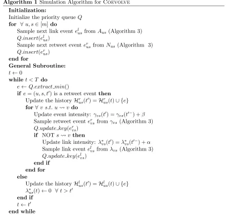
Algorithm 1 Simulation Algorithm forCoevolve
Initialization:
Initialize the priority queue Q
for ∀ u, s∈[m]do
Sample next link eventelus fromAus (Algorithm 3)
Q.insert(elus)
Sample next retweet event er
us fromNus (Algorithm 3)
Q.insert(erus)
end for
General Subroutine:
t←0
while t < T do
e← Q.extract min()
if e= (u, s, t0) is a retweet eventthen
Update the history Hr
us(t0) =Hrus(t)∪ {e}
for ∀v s.t. u v do
Update event intensity: γvs(t0) =γvs(t0−) +β
Sample retweet event ervs from γvs (Algorithm 3)
Q.update key(er
vs) if NOTs v then
Update link intensity: λ∗vs(t0) =λ∗vs(t0−) +α
Sample link eventelvs fromλvs (Algorithm 3)
Q.update key(elvs)
end if end for else
Update the history Hl
us(t0) =Hlus(t)∪ {e}
λ∗us(t)←0 ∀ t > t0
end if
t←t0
end while
As the results of this section are general and can be applied to simulate any
multi-dimensional point process model we abuse the notation a little bit and representU (possibly
inter-dependent) point processes by U intensity functions λ∗1, . . . , λ∗U. In the specific case
of simulating coevolutionary dynamics we have U = m2 +m(m−1) were the first and
second terms are the number information diffusion and link creation processes, respectively. Figure 7 illustrates the way in which both algorithms differ. The new algorithm has the following steps:
1. Initialization: Simulate each dimension separately and find their next sampled event time.
Algorithm 2 Efficient Intensity Computation
Global Variabels:
Last time of intensity computation: t
Last value of intensity computation: I Initialization:
t←0
I←µ
functionget intensity(t0)
I0←(I−µ) exp(−ω(t0−t)) +µ
t←t0
I←I0
returnI end function
Algorithm 3 1-D next event sampling
Input: Current time: t
Output: Next event time: s
s←t
ˆ
λ←λ∗(s) (Algorithm 2)
while s < T do
g∼Exponential(ˆλ)
s←s+g
¯
λ←λ∗(s) (Algorithm 2)
Rejection test:
d∼U nif orm(0,1)
if d׈λ <λ¯ then
return s
else
ˆ
λ= ¯λ
end if end while return s
3. Update: Recalculate the intensities of the dimensions that are affected by this ap-proved sample and re-sample only their next event. Then go to step 2.
Note that, events are sampled one by one; After each event, the intensities of affected dimen-sions are recomputed and fixed. This means that, the history is fixed and the dimendimen-sions of the Hawkes process become independent (just until the next event). We take next sample. Then, we make the necessary updates in the intensity functions to capture the influence of dimensions on each other. Therefore, each dimension can be thought independent until next sample is drawn because the intensity function is known.
Lemma 1 Assume we haveU independent non-homogeneous Poisson processes with
inten-sity λ∗1(τ), . . . , λU∗(τ). Take random variable τu equal to the time of process u’s first event
after time t. Define τmin= min1≤u≤U{τu} and umin = argmin1≤u≤U{τu}. Then,
(a) τmin is the first event after timet of the Poisson process with intensity λ∗sum(τ). In other words, τmin has the same distribution as the next event (t0) in Ogata’s algorithm.
(b) umin follows the conditional distribution P(umin =u|τmin =x) = λ∗U(x) λ∗
sum(x). I.e. the dimension firing the event comes from the same distribution as the one in Ogata’s algorithm.
Given the above Lemma, we can now prove that the distribution of the samples generated by the proposed algorithm is identical to the one generated by Ogata’s method.
Theorem 2 The sequence of samples from Ogata’s algorithm and our proposed algorithm follow the same distribution.
It’s noteworthy that the dimensions are not independent, but their dependency is consid-ered in the update stage. Until the next update happens they can be considconsid-ered independent because their intensity function is determined and fixed.
This new algorithm is specially suitable for the structure of our inter-coupled processes. Since social and information networks are typically sparse, every time we sample a new node (or link) event from the model, only a small number of intensity functions in the local
neighborhood of the node (or the link), will change. This number is ofO(d) wheredis the
maximum number of followers/followees per node. As a consequence, we can reuse most of the individual samples for the next overall sample. Moreover, we can find which intensity
function has the minimum sample time inO(logm) operations using a heap priority queue.
The heap data structure will help maintain the minimum and find it in logarithmic time
with respect to the number of elements therein. Therefore, we have reduced an O(nm)
factor in the original algorithm to O(dlogm).
Finally, we exploit the properties of the exponential function to update individual
inten-sities for each new sample inO(1). For simplicity consider a Hawkes process with intensity
λ∗(t) =µ+P
ti∈Htαexp(−ω(t−ti)). Note that both link creation and information diffusion
processes have this structure. Now, letti < ti+1 be two arbitrary times, we have
λ∗(ti+1) = (λ∗(ti)−µ) exp(−ω(ti+1−ti)) +µ. (23)
It can be readily generalized to the multivariate case too. Therefore, we can compute the current intensity without explicitly iterating over all previous events. As a result we can
change anO(n) factor in the original algorithm toO(1). Furthermore, the exponential kernel
also facilitates finding the upper bound of the intensity since it always lies at the beginning of one of the processes taken into consideration. Algorithm 2 summarizes the procedure to compute intensities with exponential kernels, and Algorithm 3 shows the procedure to sample the next event in each dimension making use of the special property of exponential triggering kernel.
The simulation algorithm is shown in Algorithm 1. By using this algorithm we reduce
the complexity fromO(n2m2) toO(ndlogm), wheredis the maximum number of followees
Algorithm 4 MM-type parameter learning forCoevolve
Input: Set of retweet events E = {eri} and link creation events A = {eli} observed in
time window [0, T)
Output: Learned parameters {µu},{αu},{ηu},{βs} Initialization:
for u←1 tom do
Initialize µu and αu randomly
end for
for u←1 tom do
ηu =
P
er
i∈EI[u=ui=si] T end for
for s←1 tom do
βs=
P
eri∈EI[s=si6=ui]
P
u∈[m]I[u6=s] P
v∈Fu(t) RT
0 κω1(t)?(Auv(t)dNvs(t))dt
end for
while not convergeddo fori←1 to nl do
νi1 =
µui µui+αuiP
v∈Fui(ti) κω2(t)?dNvs(t)
t=ti
νi2 =
αuiP
v∈Fui(ti) κω2(t)?dNvs(t)
t=ti
µui+αuiP
v∈Fui(ti) κω2(t)?dNvs(t)
t=ti
end for
foru←1 to m do
µu =
P
el i∈AI
[u=ui]νi1 P
s∈[m] RT
0 (1−Aus(t))dt
αu =
P
eli∈AI[u=ui]νi2
P
s∈[m] RT
0 (1−Aus(t))(κω2(t)?dNus(t))dt
end for end while
interleaving fashion, since every new retweet event will modify the intensity for link creation and vice versa.
5. Efficient Parameter Estimation from Coevolutionary Events
In this section, we first show that learning the parameters of our proposed model reduces to solving a convex optimization problem and then develop an efficient, parameter-free Minorization-Maximization algorithm to solve such problem.
5.1 Concave Parameter Learning Problem
Given a collection of retweet events E ={eri} and link creation events A = {eli} recorded
within a time window [0, T), we can easily estimate the parameters needed in our model
of these events using Equation (7), i.e.,
L({µu},{αu},{ηu},{βs}) =
X
er i∈E
log γu∗isi(ti)
− X
u,s∈[m]
Z T
0
γus∗ (τ)dτ
| {z }
tweet / retweet
+ X
el i∈A
log λ∗uisi(ti)
− X
u,s∈[m]
Z T
0
λ∗us(τ)dτ
| {z }
links
.
(24)
For the terms corresponding to retweets, the log term sums only over the actual observed events while the integral term actually sums over all possible combination of destination and source pairs, even if there is no event between a particular pair of destination and source. For such pairs with no observed events, the corresponding counting processes have essentially
survived the observation window [0, T), and the term−RT
0 γ
∗
us(τ)dτ simply corresponds to
the log survival probability. The terms corresponding to links have a similar structure.
Once we have an expression for the joint log-likelihood of the retweet and link creation events, the parameter learning problem can be then formulated as follows:
minimize{µu},{αu},{ηu},{βs} −L({µu},{αu},{ηu},{βs})
subject to µu≥0, αu ≥0, ηu ≥0, βs≥0 ∀u, s∈[m].
(25)
Theorem 3 The optimization problem defined by Equation (25) is jointly convex.
5.2 Efficient Minorization-Maximization Algorithm
Since the optimization problem is jointly convex with respect to all the parameters, one can simply take any convex optimization method to learn the parameters. However, these methods usually require hyper parameters like step size or initialization, which may sig-nificantly influence the convergence. Instead, the structure of our problem allows us to develop an efficient algorithm inspired by previous work (Zhou et al., 2013a,b; Xu et al., 2016), which leverages Minorization Maximization (MM) (Hunter and Lange, 2004) and is parameter free and insensitive to initialization.
Our algorithm utilizes Jensen’s inequality to provide a lower bound for the second log-sum term in the log-likelihood given by Equation (24). More specifically, consider a set of
arbitrary auxiliary variable νij, where 1 ≤ i ≤ nl, j = 1,2 and nl is the number of link
events,i.e.,nl=|A|. Further, assume these variables satisfy
∀ 1≤i≤nl: νi1, νi2 ≥0, νi1+νi2= 1. (26)
Lemma 4 The log-likelihood in Equation (24) is lower-bownded as follows: L≥L0 =X
er i∈E
I[ui =si] log (ηui) +
X
er i∈E
I[ui6=si] log(βsi)
+ X
er i∈E
I[ui6=si] log
X
v∈Fui(ti)
κω1(t)?(Auiv(t) dNvsi(t))
t=ti
− X
u,s∈[m]
ηuT+βs
X
v∈Fu(t)
Z T
0
κω1(t)?(Auv(t) dNvs(t))dt
+ X
el i∈A
νi1log(µui) +νi2log(αui) +νi2log
X
v∈Fui(ti)
κω2(t)? dNvs(t)
t=ti
− X
el i∈A
νi1log(νi1) +νi2log(νi2)
− X
u,s∈[m]
µu
Z T
0
(1−Aus(t))dt+αu
Z T
0
(1−Aus(t))(κω2(t)? dNus(t))dt.
(27)
Given the above lemma, by taking the gradient of the lower-bound with respect to the parameters, we can find the closed form updates to optimize the lower-bound:
ηu =
P
er
i∈EI[u=ui =si]
T (28)
βs =
P
er
i∈EI[s=si 6=ui]
P
u∈[m]I[u6=s]
P
v∈Fu(t)
RT
0 κω1(t)?(Auv(t)dNvs(t)) dt
(29)
µu =
P
el
i∈AI[u=ui]νi1
P
s∈[m]
RT
0 (1−Aus(t))dt
(30)
αu=
P
el
i∈AI[u=ui]νi2
P
s∈[m]
RT
0 (1−Aus(t))(κω2(t)? dNus(t))dt
. (31)
Finally, although the lower bound is valid for every choice ofνij satisfying Equation (26),
by maximizing the lower bound with respect to the auxiliary variables we can make sure that the lower bound is tight:
maximize{νij} L
0({µ
u},{αu},{ηu},{βs},{νij})
subject to νi1+νi2 = 1 ∀i: 1≤i≤nl
νi0, νi1 ≥0 ∀i: 1≤i≤nl.
(32)
Fortunately, the above constrained optimization problem can be solved easily via Lagrange multipliers, which leads to closed form updates:
νi1=
µui
µui+αui
P
v∈Fui(ti) κω2(t)? dNvs(t)
t=ti
(33)
νi2=
αui
P
v∈Fui(ti) κω2(t)? dNvs(t)
t=t
i
µui+αui
P
v∈Fui(ti) κω2(t)? dNvs(t)
t=ti
. (34)
It’s notable that, the maximum likelihood is prone to fall into overfitting, therefore, there is a wealth of research on how to add sparsity constraints like low rank or group sparsity regularizers (Zhou et al., 2013a) or via suitable conjugate prior (Linderman and Adams, 2014). The ideas on the next section are applicable with some modification to the case that the aforementioned ideas are utilized to improve the naive solution of the maximum likelihood.
6. Properties of Simulated Co-evolution, Networks and Cascades
In this section, we perform an empirical investigation of the properties of the networks and information cascades generated by our model. In particular, we show that our model can generate co-evolutionary retweet and link dynamics and a wide spectrum of static and temporal network patterns and information cascades.
6.1 Simulation Settings
Throughout this section, if not said otherwise, we simulate the evolution of a 8,000-node network as well as the propagation of information over the network by sampling from our model using Algorithm 1. We set the exogenous intensities of the link and diffusion events
toµu =µ= 4×10⁻⁶ and ηu=η= 1.5 respectively, and the triggering kernel parameter to
ω1 =ω2 = 1. The parameterµdetermines the independent growth of the network—roughly
speaking, the expected number of links each user establishes spontaneously before timeT is
µT. Whenever we investigate a static property, we choose the same sparsity level of 0.001.
The specific range of values we utilized in the current and the next section are such that the process remains stationary and doesn’t blow up (Hawkes, 1971). Furthermore, the range of parameters are chosen such that all the results could be reported in a unified scale.
6.2 Retweet and Link Coevolution
Figures 8(a,b) visualize the retweet and link events, aggregated across different sources, and the corresponding intensities for one node and one realization, picked at random. Here, it is already apparent that retweets and link creations are clustered in time and often follow each other. Further, Figure 8(c) shows the cross-covariance of the retweet and link creation
intensity, computed across multiple realizations, for the same node,i.e., iff(t) andg(t) are
two intensities, the cross-covariance is a function h(τ) =R
f(t+τ)g(t)dt. It can be seen
that the cross-covariance has its peak around 0,i.e., retweets and link creations are highly
correlated and co-evolve over time. For ease of exposition, we illustrated co-evolution using one node, however, we found consistent results across nodes.
6.3 Degree Distribution
Empirical studies have shown that the degree distribution of online social networks and microblogging sites follow a power law (Chakrabarti et al., 2004; Kwak et al., 2010), and argued that it is a consequence of the rich get richer phenomena. The degree distribution
of a network is a power law if the expected number of nodes md with degree dis given by
md ∝d−γ, where γ > 0. Intuitively, the higher the values of the parameters α and β, the
0 20 40 60 Event occurrence time
Spike trains
Retweet Link
0 20 40 60
0 0.6
Event occurrence time
Intensity
Retweet Link
−50 0 50
0 2 4
Cross covariance
Lag
(a) (b) (c)
Figure 8: Coevolutionary dynamics for synthetic data; (a) Spike trains of link and retweet events; (b) Link and retweet intensities with an exponentially decaying kernel; (c) Cross covariance of link and retweet intensities: The peak around 0 shows the coupling of retweet and link events.
100 101
100
102
104
Data Power−law fit Poisson fit
100 101
100
102
104
Data Power−law fit Poisson fit
100 101
100
102
104
Data Power−law fit Poisson fit
100 101 102
100
102
104
Data Power−law fit Poisson fit
(a)β = 0 (b)β= 0.001 (c) β= 0.1 (d)β = 0.8
100 101
100 102 104
Data Power−law fit Poisson fit
100 101
100 102 104
Data Power−law fit Poisson fit
100 101 102
100
102
104
Data Power−law fit Poisson fit
100 101 102
100 102 104
Data Power−law fit Poisson fit
(a)α= 0 (b) α= 0.05 (c)α= 0.1 (d) α= 0.2
Figure 9: Degree distributions when network sparsity level reaches 0.001 for differentβ (α)
values and fixedα= 0.1 (β = 0.1) are shown in top (bottom) row. By varying the
value ofβ (α) the degree distributions spans from random to scale-free networks
illustrating the flexibility of the framework to model real-world networks.
grows more locally. Interestingly, the lower their values, the closer the distribution to an
Erdos-Renyi random graph (Erdos and R´enyi, 1960), because, the edges are added almost
uniformly and independently without influence from the local structure. Figure 9 confirms
this intuition by showing the degree distribution for different values ofβ and α.
6.4 Small (shrinking) Diameter
5 10 x 10−4 0
40 80
diameter
sparsity β=0 β=0.05 β=0.1 β=0.2
5 10
x 10−4 0
40 80
diameter
sparsity α=0 α=0.001 α=0.1 α=0.8
0 0.1 0.2
0 0.15 0.3
β
clustering coefficient
0 0.75 1.5
0 0.15 0.3
α
clustering coefficient
(a) Diameter, α= 0.1 (b) Diameter,β = 0.1 (c) CC,α= 0.1 (d) CC, β = 0.1
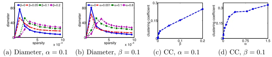
Figure 10: Diameter and clustering coefficient for network sparsity 0.001; (a,b) The
diame-ter against sparsity over time for fixedα = 0.1, and for fixedβ = 0.1 respectively;
(c,d) The clustering coefficient (CC) againstβ and α, respectively.
over time for different values ofαandβ. Although at the beginning, there is a short increase
in the diameter due to the merge of small connected components, the diameter decreases as
the network evolves. Moreover, larger values ofα orβ lead to higher levels of local growth
in the network and, as a consequence, slower shrinkage. Here, nodesarrive to the network
when they follow (or are followed by) a node in the largest connected component.
6.5 Clustering Coefficient
Triadic closure (Granovetter, 1973; Leskovec et al., 2008; Romero and Kleinberg, 2010) has been often presented as a plausible link creation mechanism. However, different social networks and microblogging sites present different levels of triadic closure (Ugander et al., 2013). Importantly, our method is able to generate networks with different levels of triadic closure, as shown by Figure 10(c-d), where we plot the clustering coefficient (Watts and Strogatz, 1998), which is proportional to the frequency of triadic closure, for different values
of α andβ.
6.6 Cascade Patterns
Our model can produce the most commonly occurring cascades structures as well as heavy-tailed cascade size and depth distributions, as observed in historical Twitter data (Goel et al., 2012). Figure 11 summarizes the results, which provide empirical evidence that the
higher theα (β) value, the shallower and wider the cascades.
7. Experiments on Model Estimation and Prediction on Synthetic Data
Oth
ers
cascade size 1 2 3 4 5 6 7 8 others
percentage
0 0.1% 1% 10% 100%
,=0 ,=0.1 ,=0.8
cascade depth 0 1 2 3 4 5 6 7 others
percentage
0 0.1% 1% 10% 100%
,=0 ,=0.1 ,=0.8
(a) (b) (c)
Oth
ers
cascade size 1 2 3 4 5 6 7 8 others
percentage
0 0.1% 1% 10% 100%
-=0.05 -=0.1 -=0.2
cascade depth 0 1 2 3 4 5 6 7 others
percentage
0 0.1% 1% 10% 100%
-=0.05 -=0.1 -=0.2
(d) (e) (f)
Figure 11: Distribution of cascade structure, size and depth for different values of α (β)
and fixed β = 0.2 (α = 0.8) on the top (bottom) row. The commom motifs of
propagation are shown in (a) and (d).
7.1 Experimental Setup
Throughout this section, we experiment with our model considering m=400 nodes. We set
the model parameters for each node in the network by drawing samples fromµ∼U(0,0.0004),
α∼U(0,0.1), η∼U(0,1.5) and β∼U(0,0.1). We then sample up to 60,000 link and infor-mation diffusion events from our model using Algorithm 1 and average over 8 different simulation runs.
7.2 Model Estimation
We evaluate the accuracy of our model estimation procedure via two measures: (i) the
relative mean absolute error (i.e., E[|x−xˆ|/x], MAE) between the estimated parameters
(x) and the true parameters (ˆx), (ii) the Kendall’s rank correlation coefficient between each
estimated parameter and its true value, and (iii) test log-likelihood. Tables 1 and 2, and Figure 12 show the rank correlation, relative error, and the log likelihood on the test data, respectively. They show that as we feed more events into the estimation procedure, the estimation becomes more accurate.
7.3 Link Prediction
Table 1: Parameter Estimation Results (Rank Correlation)
# Events α β η µ
5×10⁴ 0.66 ±0.05 0.82±0.05 0.81 ±0.05 0.72 ±0.03
4×10⁴ 0.58 ±0.03 0.79±0.04 0.72 ±0.05 0.65 ±0.03
3×10⁴ 0.49 ±0.05 0.76±0.04 0.66 ±0.04 0.58 ±0.05
2×10⁴ 0.38 ±0.05 0.65±0.05 0.54 ±0.05 0.47 ±0.05
1×10⁴ 0.24 ±0.03 0.43±0.05 0.29 ±0.04 0.26±0.04
Table 2: Parameter Estimation Results (Relative Error)
# Events α β η µ
5×10⁴ 0.25 ±0.05 0.1±0.04 0.16 ±0.05 0.18 ±0.05
4×10⁴ 0.31 ±0.05 0.17±0.05 0.24 ±0.03 0.28 ±0.06
3×10⁴ 0.47 ±0.04 0.32±0.04 0.35 ±0.04 0.39 ±0.05
2×10⁴ 0.65 ±0.05 0.49±0.04 0.55 ±0.04 0.57 ±0.05
1×10⁴ 0.86 ±0.05 0.71±0.04 0.75 ±0.06 0.79 ±0.05
state of the art methods, which we denote as TRF (Antoniades and Dovrolis, 2015) and WENG (Weng et al., 2013).
Central to TRF model is the notion of TRF event: When a followerL∈ F(R) receives a
retweet ofS throughR,Lcan decide to followS directly. They call this sequence a
Tweet-Retweet-Follow (TRF) event, and refer to its three main actors as SpeakerS, Repeater R,
and Listener L. In addition to characterizing and identifying such events, TRF measures
the probability of creating a link from a source at a given time by simply computing the proportion of new links created from the source over all total created links up to the given time. More specifically, it estimates the probability of new link as follows. Consider a tweet
of Speaker S at time ts . Suppose that this tweet is not retweeted by any of the followers
of S in the period [ts, ts+ ∆]. Let Φ(S, ts) be the set of followers of followers ofS that are
not directly following S atts. The exogenous probability of of followingS is:
PEXO=
|L:L∈Φ(S, ts), L∈ F(S, ts+ ∆|
|Φ(S, ts)|
. (35)
Similarly, consider a tweet of SpeakerS at timets that has been retweeted by a follower of
S, referred to as RepeaterR, at timetr > ts . Let ΦR(S, tr) be the subset of Φ(S, tr) that
includes only followers ofR. The endogenous probability of followingS is:
PEN D=
|L:L∈ΦR(S, tr), L∈ F(S, tr+ ∆|
|ΦR(S, tr)|
. (36)
And the probability of following S is simply PEXO+PEN D.
1 3 5
x 104 −2.8
−2.2 −1.6
x 105
# events
PredLik
Figure 12: Performance of model estimation for the synthetic network reported in Log-likelihood on unseen test data.
1 3 5
x 104 25
50
# events
AvgRank
COEVOLVE TRF WENG
1 3 5
x 104
0 0.2 0.4
# events
Top−1
COEVOLVE TRF WENG
1 3 5
x 104
0 10 20
# events
AvgRank
COEVOLVE HAWKES
1 3 5
x 104 0
0.3 0.6
# events
Top−1
COEVOLVE HAWKES
(a) Links: AR (b) Links: Top-1 (c) Activity: AR Activity: Top-1
Figure 13: Prediction performance of future links and activities for a 400-node synthetic network on the test unseen data. The accuracy is reported by means of average rank (AR) and success probability that the true events rank among the top-1 events (Top-1).
Origin: follow a randomly selected origin; Traffic shortcut: follow a randomly selected grandparent or origin. Then, they parameterize the the probability of using a strategy and learned the it using maximum likelihood. Because of the contribution of multiple terms in the log-likelihood expression (due to the mixed effects of strategies) they numerically explore the values of parameters in the unit square to maximize the log-likelihood.
Here, we evaluate the performance by computing the probability of all potential links using our model, TRF and WENG. In our model, the intensity gives us a measure of how likely a link will be created at a specific point of time. The higher the intensity, the more likely the connection. Therefore, we can sort the future events based on the likelihood of happening. Then, we compute (i) the average rank of all true (test) events in our sorted list (AvgRank) and, (ii) the success probability that the true (test) events rank among the top-1 potential events at each test time (Top-1). Figure 13 summarizes the results, where we trained our model with an increasing number of events. Our model outperforms both TRF and WENG for a significant margin.
7.4 Activity Prediction
0 50 100 Event occurrence time
Spike trains
Retweet Link
0 50 100
0 0.4 0.8
Event occurrence time
Intensity
Retweet Link
0 20 40 60 80
Event occurrence time
Spike trains
Retweet Link
0 20 40 60 80
0 0.5 1
Event occurrence time
Intensity
Retweet Link
(a) (b) (c) (d)
0 20 40 60
Event occurrence time
Spike trains
Retweet Link
0 20 40 60
0 0.5 1
Event occurrence time
Intensity
Retweet Link
0 20 40
Event occurrence time
Spike trains
Retweet Link
0 20 40
0 0.3 0.6
Event occurrence time
Intensity
Retweet Link
(e) (f) (g) (h)
Figure 14: Link and retweet behavior of 4 typical users in the real-world data set. Panels (a,c,e,g) show the spike trains of link and retweet events and Panels (b,d,f,h) show the estimated link and retweet intensities with exponential decaying kernel.
part. For the Hawkes baseline, we take a snapshot of the network right before the prediction
time, and use all historical retweeting events to fit the model and finding (auv)u,v∈[m] and
(ηu)u∈[m] similar to previous works (Farajtabar et al., 2014). Here, each user u performs
activity with intensity
γu(t) =ηu+
X
v∈Fu(t)
auv κω1(t)? dNv(t). (37)
Now, we have two Hawkes process based models, Coevolve, which considers information
propagation coevolved with the link creation process, and the baseline Hawkes model which only contains the information propagation part to model activities. Similar to the link prediction we used the intensity to measure how likely is an event. We can sort future events according to their probability. Then, we evaluate the performance via the same two measures as in the link prediction task and summarize the results in Figure 13 against an increasing number of training events. Please refer to the previous subsection to learn about the measures used here. The results show that, by modeling the network evolution, our model performs significantly better than the baseline.
8. Experiments on Coevolution and Prediction on Real Data
−1000 0 100 2
4 6
Lag
Cross covariance
Estimated Empirical
−1000 0 100
2 4
Lag
Cross covariance
Estimated Empirical
−1000 0 100
2 4 6
Lag
Cross covariance
Estimated Empirical
−1000 0 100
2 4 6
Lag
Cross covariance
Estimated Empirical
Figure 15: Empirical and simulated cross covariance of link and retweet intensities for four typical users.
and, by doing so, it predicts retweet and link creation events more accurately than several alternatives.
8.1 Data Set Description & Experimental Setup
We use a data set that contains both link events as well as tweets/retweets from millions of Twitter users (Antoniades and Dovrolis, 2015). In particular, the data set contains data from three sets of users in 20 days; nearly 8 million tweet, retweet, and link events by more
than 6.5 million users. The first set of users (8,779 users) are source nodes s, for whom all
their tweet times were collected. The second set of users (77,200 users) are the followers of the first set of users, for whom all their retweet times (and source identities) were collected. The third set of users (6,546,650 users) are the users that start following at least one user in the first set during the recording period, for whom all the link times were collected.
In our experiments, we focus on all events (and users) during a 10-day period (Sep 21 2012 - 30 Sep 2012) and used the information before Sep 21 to construct the initial social network (original links between users). We model the co-evolution in the second 10-day period using our framework. More specifically, in the coevolution modeling, we have 5,567 users in the first layer who post 221,201 tweets. In the second layer 101,465 retweets are generated by the whole 77,200 users in that interval. And in the third layer we have 198,518 users who create 219,134 links to 1978 users (out of 5567) in the first layer.
We split events into a training set (covering 85% of the retweet and link events) and a
test set (covering the remaining 15%) according to time, i.e., all events in the training set
occur earlier than those in the test set. We then use our model estimation procedure to fit the parameters from an increasing proportion of events from the training data.
8.2 Retweet and Link Coevolution
1 500 1000 0
0.75 1.5
Index of users
Parameters
mcc α β
Figure 16: Empirical cross covariance and learned model parameters for 1,000 users, picked
at random. The x-axis indexes the users while theirα,β and the empirical cross
covariance are shown in different colors on the y-axis.
their peak around 0, i.e., retweets and link creations are highly correlated and co-evolve
over time. For ease of exposition, as in Section 6, we illustrated co-evolution using four nodes, however, we found consistent results across nodes.
To further verify that our model can capture the coevolution, we compute the average
value of the empirical cross covariance function, denoted by mcc, per user. Intuitively, one
could expect that our model estimation method should assign higher α and/orβ values to
users with high mcc. Figure 16 confirms this intuition on 1,000 users, picked at random.
Whenever a user has high α and/or β value, she exhibits a high cross covariance between
her created links and retweets.
8.3 Link Prediction
We use our model to predict the identity of the source for each test link event, given the historical (link and retweet) events before the time of the prediction, and compare its performance with the same two state of the art methods as in the synthetic experiments, TRF (Antoniades and Dovrolis, 2015) and WENG (Weng et al., 2013).
We evaluate the performance by computing the probability of all potential links using different methods, and then compute (i) the average rank of all true (test) events (AvgRank) and, (ii) the success probability (SP) that the true (test) events rank among the top-1
potential events at each test time (Top-1). We summarize the results in Figure
17(a-b), where we consider an increasing number of training retweet/tweet events. Our model
outperforms TRF and WENG consistently. For example, for 8·104 training events, our
model achieves a SP 2.5x times larger than TRF and WENG.
8.4 Activity Prediction
# events ×105
1 3 5
AvgRank
10 70 140
COEVOLVE TRF WENG
# events ×105
1 3 5
Top1
0 0.1 0.2
COEVOLVE TRF WENG
# events ×105
1 3 5
AvgRank
40 80
COEVOLVE HAWKES
# events ×105
1 3 5
Top1
0 0.15 0.3
COEVOLVE HAWKES
(a) Links: AR (b) Links: Top-1 (c) Activity: AR Activity: Top-1
Figure 17: Prediction performance in the Twitter data set by means of average rank (AR) and success probability that the true (test) events rank among the top-1 events (Top-1).
0 5 10
0 5 10
Q. observed time samples
Q. exponential distribution
0 5 10
0 5 10 15
Q. observed time samples
Q. exponential distribution
(a) Link process (b) Retweet process
Figure 18: Quantile plots of the intensity integrals from the real link and retweet event time. The alignment of blue dots (empirical) and red ones (theoretical) shows the suitability of our model in representing observed traces of activities in Twitter.
8.5 Model Checking
Given all the subsequent event times generated using a Hawkes process, i.e., ti and ti+1,
according to the time changing theorem (Daley and Vere-Jones, 2007), the intensity integrals Rti+1
ti λ(t)dtshould conform to the unit-rate exponential distribution. Figure 18 presents the
quantiles of the intensity integrals computed using intensities with the parameters estimated from the real Twitter data against the quantiles of the unit-rate exponential distribution. It clearly shows that the points approximately lie on the same line, giving empirical evidence that a Hawkes process is the right model to capture the real dynamics.
9. Related Work
In this section, we survey related works in modeling temporal networks followed by a sub-section on co-evolution dynamics. Next, we review the literature on information diffusion models. Finally, we conclude this section by works that are closely related and are developed for almost the same goal.
in the social network modeling community (Goldenberg et al., 2010). However, most of these models use timing information as discrete indices. The dynamics of the resulting time-discretized model can be quite sensitive to the chosen discretization time steps; Too coarse a discretization will miss important dynamic features of the process, and too fine a discretization will increase the computational and inference costs of the algorithms. In contrast, the events we try to model tend to be asynchronous with a number of different time scales. Recently, Snijders and Luchini (2006) used a Cox-intensity Poisson model with exponential random graphs to model friendship dynamics. Brandes et al. (2009) extended this model to the temporal sequence of interactions that take place in the social network, but with insufficient model flexibility, and limited scalability. However, these works largely fail to model the interdependency between events generated by different users, which is one of the focuses of our proposed framework. Most of this line of work is summarized in a recent survey (Holme, 2015), with a short section devoted to point process based approaches.
Co-evolution Dynamics. In machine learning and several other communities, both the dynamics on the network and the dynamics of the network have been extensively studied, and combining the two is a natural next step. For example, Bhattacharya et al. (2015) claimed that content generation in social networks is influenced not just by their personal
features like age and gender, but also by their social network structure. Furthermore,
research has been done to address the co-evolution problems, for example, in the complex
network literature, under the name ofadaptive system(Gross and Blasius, 2008). The main
premise is that the evolution of the topology depends on the dynamics of the nodes in the network, and a feedback loop can be created between the two, which allows dynamical exchange of information. In a different context, epidemiologists have found that nodes may rewire their links to try to avoid contact with the infected ones (Gross et al., 2006). Co-evolutionary models have been also developed for collective opinion formation, investigating whether the coevolutionary dynamics will eventually lead to consensus or fragmentation of the population (Zschaler et al., 2012). However, this line of research tends to be less data-driven.Moreover, although the general nonlinear dynamic-system based methods usually address co-evolutionary phenomena that are macroscopic in nature, they lack the inference power of statistical generative models which are more adapted to teasing out microscopic details from the data. Finally, we would also like to mention a different line of research exemplified by the actor-oriented models developed by Snijders (2014), where a continuous-time Markov chain on the space of directed networks is specified by local node-centric probabilistic link change rules, and MCMC and method of moments are used for parameter estimation. Hawkes processes we used are generally non-Markovian and making use of event history far into the past.