Learning Partial Policies to Speedup MDP Tree Search
via Reduction to I.I.D. Learning
Jervis Pinto
School of EECS, Oregon State University, Corvallis OR 97331 USA
Alan Fern
School of EECS, Oregon State University, Corvallis OR 97331 USA
Editor:Michael Bowling
Abstract
A popular approach for online decision-making in large MDPs is time-bounded tree search. The effectiveness of tree search, however, is largely influenced by the action branching factor, which limits the search depth given a time bound. An obvious way to reduce action branching is to consider only a subset of potentially good actions at each state as specified by a provided partial policy. In this work, we consider offline learning of such partial policies with the goal of speeding up search without significantly reducing decision-making quality. Our first contribution consists of reducing the learning problem to set learning. We give a reduction-style analysis of three such algorithms, each making different assumptions, which relates the set learning objectives to the sub-optimality of search using the learned partial policies. Our second contribution is to describe concrete implementations of the algorithms within the popular framework of Monte-Carlo tree search. Finally, the third contribution is to evaluate the learning algorithms on two challenging MDPs with large action branching factors. The results show that the learned partial policies can significantly improve the anytime performance of Monte-Carlo tree search.
Keywords: online sequential decision-making, partial policy, partial policy learning, imitation learning, Monte-Carlo tree search, reductions
1. Introduction
Online sequential decision-making involves selecting actions in order to optimize a long-term per-formance objective while meeting practical decision-time constraints. In many environments, in-cluding Chess, Go, computer networks, automobiles and aircraft, it is possible to obtain simulators or learn an accurate model of the environment, whereas in others, no such simulator or model is available. A common approach in both cases is to use learning techniques such as reinforcement learning (RL) (Sutton and Barto, 1998) or imitation learning (Pomerleau, 1989; Sammut et al., 1992) in order to learn reactive policies, which can be used to quickly map any state to an action. While reactive policies support fast decision making, for many complex problems, it can be difficult to represent and learn high-quality reactive policies. For example, in games such as Chess, Go, and other complex problems, the best learned reactive policies are significantly outperformed by the best approaches based on look-ahead search (Gelly and Silver, 2007; Veness et al., 2009; Silver et al., 2016). As another example, recent work has shown that effective reactive policies can be learned
c
for playing a variety of Atari video games using both RL (Mnih et al., 2013) and imitation learning (Guo et al., 2014). However, the performance of these reactive policies are easily outperformed or equaled by a vanilla lookahead planning agent (Guo et al., 2014).
Faced with the choice of a planning agent versus a (model-free) learning agent, a practitioner must consider two key factors. The first is the non-trivial expense of obtaining a simulator or learn-ing a model. The second is that the plannlearn-ing agent requires significantly more time per decision. That is, even when a simulator is available, the computational expense may not be practical for certain applications, including real-time Atari game play.
This paper attempts to make progress in the region between fast reactive decision making and slow lookahead search, when a simulator or model of the world is available. In particular, we study algorithms for learning to improve the anytime performance of lookahead search, allowing for more effective deliberative decisions to be made within practical time bounds. Lookahead tree search constructs a finite-horizon lookahead tree using a (possibly stochastic) model or simulator in order to estimate action values at the current state. A variety of algorithms are available for building such trees, including instances of Monte-Carlo Tree Search (MCTS) such as UCT (Kocsis and Szepesv´ari, 2006), Sparse Sampling (Kearns et al., 2002), and FSSS (Walsh et al., 2010), along with model-based search approaches such as RTDP (Barto et al., 1995) and AO* (Blai and Hector, 2012). However, under practical time constraints (e.g., one second per root decision), the performance of these approaches strongly depends on the action branching factor. In non-trivial MDPs, the number of possible actions at each state is often considerable, which greatly limits the feasible search depth. An obvious way to address this problem is to provide prior knowledge for explicitly pruning bad actions from consideration. In this paper, we consider the offline learning of such prior knowledge in the form of partial policies1.
A partial policy is a function that quickly returns an action subset for each state and can be integrated into search by pruning away actions not included in the subsets. Thus, a partial policy can significantly speedup search if it returns small action subsets, provided that the overhead for applying the partial policy is small enough. If those subsets typically include high-quality actions, then we might expect little decrease in decision-making quality. Although learning partial policies to guide tree search is a natural idea, it has received surprisingly little attention, both in theory and practice. In this paper we formalize this learning problem from the perspective of “speedup learning”. We are provided with a distribution over search problems in the form of a root state distribution and a search depth bound. The goal is to learn partial policies that significantly speedup depth Dsearch, while bounding the expected regret of selecting actions using the pruned search versus the original search method that does not prune.
In order to solve this learning problem, there are at least two key choices that must be made: 1) Selecting a training distribution over states arising in lookahead trees, and 2) Selecting a loss function that the partial policy is trained to minimize with respect to the chosen distribution. The key contribution of our work is to consider a family of reduction-style algorithms that answer these questions in different ways. In particular, we consider three algorithms that reduce partial pol-icy learning to set learning problems, characterized by choices for (1) and (2). The set learning problems are further reduced to cost-sensitive binary classification. Our main results bound the sub-optimality of tree search using the learned partial policies in terms of the expected loss of the supervised learning problems. Interestingly, these results for learning partial policies mirror similar
reduction-style results for learning (complete) policies via imitation (Ross and Bagnell, 2010; Syed and Schapire, 2010; Ross et al., 2011).
We empirically evaluate our algorithms in the context of learning partial policies to speedup MCTS in two challenging domains with large action branching factors: 1) a real-time strategy game, Galcon and 2) a classic dice game, Yahtzee. The results show that using the learned partial policies to guide MCTS leads to significantly improved anytime performance in both domains. Furthermore, we show that several other existing approaches for injecting knowledge into MCTS are not as effective as using partial policies for action pruning and can often hurt search performance rather than help.
2. Problem Setup
We consider sequential decision-making in the framework of Markov Decision Processes (MDPs). An MDP is a tuple(S, A, P, R), whereSis a finite set of states,Ais a finite set of actions,P(s0|s, a)
is the transition probability of arriving at states0 after executing actionain states, andR(s, a) ∈
[0,1]is the reward function giving the reward of taking actionain states. In environments where the reward is non-deterministic (but still stationary), R(s, a) is taken to be the expected value. The typical goal in MDP planning and learning is to compute a policy for selecting an action in any state, such that following the policy (approximately) maximizes some measure of long-term expected reward. For example, two popular choices are maximizing the expected finite-horizon total reward or expected infinite-horizon discounted reward.
In practice, regardless of the long-term reward measure, for large MDPs, the offline compu-tation of high-quality policies over all environment states is impractical. In such cases, a popular action-selection approach is online tree search, where at each encountered environment state, a time-bounded search is carried out in order to estimate action values. Note that this approach requires the availability of either an MDP model or a simulator in order to construct search trees. In this paper, we assume that a model or simulator is available and that online tree search has been chosen as the action selection mechanism. Next, we formally describe the paradigm of online tree search, introduce the notion of partial policies for pruning tree search, and then formulate the problem of offline learning of such partial policies.
2.1 Online Tree Search
Throughout this paper, we will focus on search that has a depth boundD. Doing so bounds the length of future action sequences to be considered. Given a states, we denote byT(s) the depth
Dexpectimax tree rooted at s. T(s)alternates between layers of state nodes and action nodes2, labeled by states and actions respectively. The children of each state node are action nodes for each action inA. The children of an action nodeawith parent labeled bysare all states s0 such that
P(s0|s, a)>0. Figure 1(a) shows an example of a depth two expectimax tree. The depth of a state node is the number of action nodes traversed from the root to reach it. Note that leaves ofT(s)will always be action nodes.
The optimal value of a state nodesat depthd, denoted byVd∗(s), is equal to the maximum value of its child action nodes, which we denote byQ∗d(s, a)for childa.Vd∗(s)andQ∗d(s, a)are formally defined next.
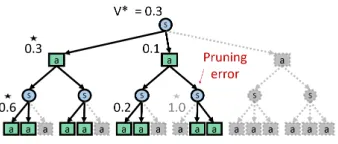
(a) Unpruned expectimax treeT(s)withD= 2 (b) PruningT withpartial policyψ gives Tψ
where a third of the actions have been pruned.
Figure 1: Unpruned and pruned expectimax trees with depthD = 2 for an MDP with |A| = 3
and two possible next states. The distributions over the transitions to the next state are uniform. The numeric values are the optimal action values Q∗. Nodes for which no value is shown haveQ∗(s, a) = 0. Nodes marked with an asterisk indicate that the node corresponds to the optimal action choice. In (b), pruning can change the value at the root if nodes on the optimal paths are incorrectly pruned.
Vd∗(s) = max
a Q
∗ d(s, a)
Q∗d(s, a) =R(s, a) if d=D−1 (1)
=R(s, a) +Es0∼P(· |s,a)Vd∗+1(s0) otherwise (2)
Equation 1 corresponds to leaf action nodes. In Equation 2, s0 ∼ P(·|s, a) ranges over the children ofa. Given these value functions, the optimal action policy for statesat depthdis
πd∗(s) = arg max
a Q
∗ d(s, a)
Given an environment states, online search algorithms such as UCT or RTDP attempt to com-pletely or partially search the treeT(s)in order to approximate the root action valuesQ∗0(s, a)well enough to identify the optimal actionπ∗0(s). It is important to note that optimality in our context is with respect to the specified search depthD, which may be significantly smaller than the number of actions that will be taken in the actual environment (e.g., the length of a full game). This is a practical necessity that is often referred to as receding-horizon control. Here we simply assume that an appropriate search depthDhas been specified and our goal is to speedup planning within that depth.
2.2 Search with a Partial Policy
One way to speedup depthDsearch is to prune actions fromT(s). In particular, if a fixed fraction
σof actions are removed from each state node, then the size of the tree would decrease by a factor of(1−σ)D, potentially resulting in significant computational savings. In this paper, we will utilize
partial policies for pruning actions. A depth D (non-stationary) partial policy ψ is a sequence
(ψ0, . . . , ψD−1)where eachψdmaps a state to an action subset. In this work, we focus exclusively
on non-stationary partial policies, rather than also considering stationary partial policies whereψi=
non-stationary in general. In addition, considering non-stationary policies allows for defining and analyzing relatively simple training algorithms as described in section 3. In some applications, however, where the planning depth is not known in advance, it may be desirable to learn stationary partial policies. Extending our work to the stationary scenario is a point of future work, which we expect can draw on ideas for learning stationary policies in imitation learning (Ross and Bagnell, 2010; Ross et al., 2011).
Given a partial policy ψand root state s, we can define a pruned treeTψ(s) that is identical
toT(s), except that each state sat depthdonly has subtrees for actions inψd(s), pruning away
subtrees for any childa /∈ ψd(s). The phrase “root state” is not to be confused with the starting
state of a sequential problem (e.g., the initial board in Chess). Rather, “root state” refers toany
state in which the search agent is required to act and must therefore place the state at the root of the search tree. Figure 1(b) shows a pruned treeTψ(s), whereψprunes away one action at each state. It
is straightforward to incorporateψinto a search algorithm by only expanding actions at state nodes that are consistent withψ.
We define the state and action values relative to Tψ(s)the same as before and let Vdψ(s)and
Qψd(s, a)denote the depthdstate and action value functions, as follows.
Vdψ(s) = max
a∈ψd(s)
Qψd(s, a)
Qψd(s, a) =R(s, a) if d=D−1
=R(s, a) +Es0∼P(· |s,a)
h
Vdψ+1(s0)i otherwise
We will denote the highest-valued, or greedy, root action ofTψ(s)as
πψ(s) = arg max
a∈ψ0(s)Q
ψ 0(s, a)
This is the root action that a depthD search procedure would attempt to return in the context of
ψ. We say that a partial policyψsubsumes a partial policyψ0 if for eachsandd,ψd0(s)⊆ ψd(s).
In this case, it is straightforward to show that for anysandd,Vdψ0(s) ≤ Vdψ(s). This is simply because planning underψallows for strictly more action choices than planning underψ0. Note that a special case of partial policies is when|ψd(s)|= 1for allsandd, which means thatψdefines a
traditional (complete) deterministic MDP policy. In this case,Vdψ andQψd represent the traditional depth dstate value and action value functions for policies. The second special case occurs at the other extreme whereψd=Afor alld. This corresponds to full-width search and we haveV∗ =Vψ
andQ∗=Qψ.
Clearly, a partial policy can reduce the complexity of search by eliminating some actions. How-ever, we are also concerned with the quality of decision-making using Tψ(s)versusT(s), which
we will quantify in terms of expected regret. The regret of selecting actionaat statesrelative to
T(s) is equal toV0∗(s)−Q∗0(s, a). Note that the regret of the optimal actionπ∗0(s) is zero. We prefer partial policies that result in root decisions with small regret over the root state distribution that we expect to encounter, while also supporting significant pruning. For this purpose, ifµ0 is a
distribution over root states, we define the expected regret ofψwith respect toµ0as
REG(µ0, ψ) =E
h
V0∗(s0)−Q∗0(s0, πψ(s0))
i
2.3 Learning Problem
We consider an offline learning setting where we are provided with a model or simulator of the MDP in order to train a partial policy that will be used later for online decision-making. As an illustrative example, consider the domain of Chess, where we wish to learn a partial policy for pruning the search tree. Our approach is to use expensive search offline to play many full games of Chess and to record the sequence of states encountered during those games. Each state encountered during actual play is called aroot stateof a search tree. The collected root states and associated trees are then used to learn a partial policy that can be used to speedup future online search.
More formally, the learning problem provides us with a distribution µ0 over root states (or a
representative sample fromµ0) and a depth boundD. In our Chess example,µ0would be a
distri-bution over the states encountered along games played using the expensive search. The intention is forµ0to be representative of the states that will be encountered during online use. In this work, we
are agnostic about howµ0 is defined for an application. A typical choice ofµ0 is the distribution
of states encountered along trajectories of a receding-horizon controller that makes decisions based on unpruned depthDsearch. We use this definition ofµ0in our experiments. This setup is closely
related to imitation learning (Syed and Schapire, 2010; Ross and Bagnell, 2010; Ross et al., 2011) since we are essentially treating unpruned, expensive search as the expert to be imitated by a pruned search. Other choices of the initial state distributionµ0 are the state distributions that arise from
more complex imitation learning algorithms such as DAGGER (Ross et al., 2011).
Givenµ0andD, our “speedup learning” goal is to learn a partial policyψwith small expected
regret REG(µ0, ψ), while providing significant pruning. That is, we want to imitate the decisions
of depthD unpruned search via a much less expensive depthD pruned search. In general, there will be a tradeoff between the potential speedup and expected regret. At one extreme, it is always possible to achieve zero expected regret by selecting a partial policy that does not prune. At the other extreme, we can remove the need for any search by learning a partial policy that always returns a single action, which corresponds to a complete policy. However, for many complex MDPs, it can be difficult to learn computationally efficient, or reactive, policies that achieve small regret. Rather, it may be much easier to learn partial policies that prune away many, but not all actions, yet still retain high-quality actions. While such partial policies lead to more search than a reactive policy, the regret may be much less.
In practice, we seek a good tradeoff between the two extremes. The tradeoff between a reactive policy versus a full depthDsearch-based policy is application-specific. Instead of specifying a par-ticular trade-off point as our learning objective, we develop learning algorithms in the next section that provide some ability to explore different points. In particular, the algorithms are associated with regret bounds in terms of supervised learning objectives that measurably vary with different amounts of pruning.
3. Learning Partial Policies
Given µ0 and D, we now develop reduction-style algorithms for learning partial policies. The
algorithms reduce partial policy learning to a sequence ofDi.i.d. supervisedset learningproblems, each producing one partial policy component ψd. Informally, a supervised set learning problem
should return. The quality of a learned set function will be evaluated in terms of a cost function that provides a measure of whether a set returned by the function contains “good” labels/actions.
More formally, the set learning problem for partial policy componentψdwill be characterized
by a pair(µd, Cd), whereµdis a distribution over states, andCdis a cost function that, for any state
sand action subsetA0 ⊆ Aassigns a prediction costCd(s, A0). The cost function is intended to
measure the quality ofA0 with respect to including actions that are high quality fors. Typically, the cost function will be a monotone decreasing set function ofA0with zero pruning having zero cost,
Cd(s, A) = 0. Note that a trivial solution to the learning problem, which achieves zero cost, would
be to learn a function that always returns the complete action setA. However, such solutions will be avoided by having the designer specify the amount of pruning that they desire, or equivalently the size of the action sets returned. Note that constraining the set to contain exactly one action would correspond to learning complete policies.
We begin by assuming the availability of a set learning algorithm called SETLEARNthat takes
three inputs, namely, a set of states drawn from µd, cost function Cd, and a pruning percentage
0< σd<1. The output of SETLEARNis a partial policy componentψdthat returns action sets that
contain at most a fraction1−σdof the available actions while attempting to minimize the expected
cost ofψdonµd. That is, the goal is to return aψdthat minimizesE[Cd(s, ψd(s))]fors∼µd. The
designer’s choice of pruning percentageσd(e.g., prune 75% of the actions in each state) is related to
the time constraints of the decision problem, with smaller time constraints requiring more pruning. Given access to SETLEARN we first present our generic reduction algorithm for learning par-tial policies in Algorithm 1. This algorithm template simply calls SETLEARN on a sequence of
Algorithm 1A template for learning a partial policyψ= (ψ0, . . . , ψD−1). The template is
instan-tiated by specifying the pairs of distributions and cost functions(µd, Cd)ford∈ {0, . . . , D−1}.
SETLEARNis a set learning algorithm that aims to minimize the expected cost of eachψdrelative
toCdandµd. σdis a pruning fraction such that SETLEARNreturns at most1−σdactions. Each
partial policyψdis a set function that maps states to action sets of size(1−σd)|A|. 1: procedurePARTIALPOLICYLEARNER({(µd, Cd)}, σd)
2: ford= 0,1, . . . , D−1do
3: Sample a training set of statesSdfromµd
4: ψd← SETLEARN(Sd, Cd, σd)
5: end for
6: returnψ= (ψ0, ψ1, . . . , ψD−1) 7: end procedure
set learning problems and returns a list of the learned partial policies. In order to instantiate this template, it is necessary to specify SETLEARNand the individual set learning problems(µd, Cd).
We defer details of our implementation of SETLEARNuntil section 4. Rather, we proceed with the definition of our learning reductions. Each reduction is specified by a particular choice of(µd, Cd),
such that we can bound the expected regret ofψ(when used for search) by the expected (i.i.d.) costs of theψdreturned by SETLEARN.
We begin with the state distributionsµd. These are specified in terms of distributions induced
by (complete) policies. In particular, given a policyπ, we letµd(π) denote the state distribution
produced by the following procedure: Draw an initial state fromµ0, executeπfordsteps and return
fromµd(π)for any providedπ. Before proceeding, we state two simple lemmas that will be used
to prove our regret bounds.
Lemma 1 If a complete policyπ is subsumed by partial policyψ, then for any initial state distri-butionµ0, REG(µ0, ψ)≤E[V0∗(s0)]−E[V0π(s0)], fors0 ∼µ0.
Proof Sinceπ is subsumed byψ, we know thatQψ0(s, πψ(s)) = Vψ
0 (s) ≥ V0π(s). Since for any
a,Q∗0(s, a) ≥ Qψ0(s, a), we have for any state s, Q∗0(s, πψ(s)) ≥ Vπ
0 (s). The result follows by
negating each side of the inequality, followed by addingV0∗(s), and taking expectations.
Thus, we can bound the regret of a learnedψif we can guarantee that it subsumes a policy whose ex-pected value has bounded sub-optimality. Our three reduction algorithms, presented below, provide different approaches for making such a guarantee.
The second lemma will be used to bound the optimality of complete polices that are sub-sumed by our learned partial policies, which then allows the application of Lemma 1. Versions of this “performance difference lemma” have been used in prior work (Kakade and Langford, 2002; Bagnell et al., 2003; Ross and Bagnell, 2014).
Lemma 2 For any two complete policiesπandπ0and any initial state distributionµ0,
EhV0π0(s0)−V0π(s0)
i
=
D−1
X
d=0
EhVdπ0(sd)−Qπ 0
d(sd, π(sd))
i
,wheresd∼µd(π0:d−1)
.
Proof Following a prior proof (Ross and Bagnell, 2014), define πdto be a policy that follows π
fordsteps and then at stepd+ 1switches to followingπ0 until the maximum depthD. Using the observations thatπ0 =π0andπD =π, we can derive the following.
EhV0π0(s0)−V0π(s0)
i
= E
"D−1 X
d=0
Vπd
0 (s0)−V
πd+1
0 (s0)
#
=
D−1
X
d=0
EVπd
0 (s0)−V
πd+1
0 (s0)
=
D−1
X
d=0
E
h
Vdπ0(sd)−Qπ 0
d(sd, π(sd))
i
,wheresd∼µd(π0:d−1)
The first equality is simply a telescoping sum. The third equality follows due the fact thatπdand
πd+1both followπfor the firstdsteps, which yields the same distribution oversd.
We will use this lemma when the reference policyπ0 is optimal, that is,π0 = π∗. Thus, the sub-optimality ofπ can be bounded by accumulating the expected sub-optimality of its action choices along trajectories generated byπ. Next, we present our three reduction algorithms, which are sum-marized in Table 1.
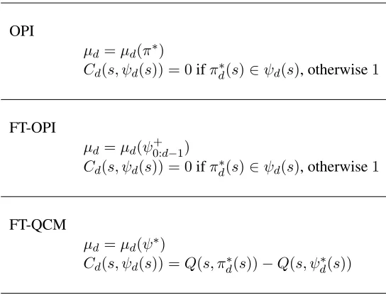
3.1 OPI : Optimal Partial Imitation
OPI
µd=µd(π∗)
Cd(s, ψd(s)) = 0ifπd∗(s)∈ψd(s), otherwise1
FT-OPI
µd=µd(ψ+0:d−1)
Cd(s, ψd(s)) = 0ifπd∗(s)∈ψd(s), otherwise1
FT-QCM
µd=µd(ψ∗)
Cd(s, ψd(s)) =Q(s, πd∗(s))−Q(s, ψd∗(s))
Table 1: Instantiations for OPI, FT-OPI and FT-QCM in terms of the template in Algorithm 1. Note thatψdis a partial policy whileπd∗, ψd+andψ∗dare complete policies.
be learned so as to maximize the probability of containing actions selected byπd∗with respect to the optimal state distributionµd(π∗). This approach is followed by our first algorithm called Optimal
Partial Imitation (OPI). In particular, Algorithm 1 is instantiated with µd = µd(π∗) (noting that
µ0(π∗) is equal toµ0 as specified by the learning problem) and Cd equal to zero-one cost. Here
Cd(s, A0) = 0ifπ∗d(s)∈A0andCd(s, A0) = 1otherwise. Note that the expected cost ofψdin this
case is equal to the probability thatψddoes not contain the optimal action. We refer to this as the
pruning error and denote it by
e∗d(ψ) = Pr
s∼µd(π∗)
(πd∗(s)∈/ψd(s)) (4)
A naive implementation of OPI is straightforward. We can generate length D trajectories by drawing an initial state fromµ0 and then selecting actions (approximately) according toπ∗d using
standard unpruned search. Defined like this, OPI has the nice property that it only requires the ability to reliably compute actions ofπ∗d, rather than requiring that we also estimate action values accurately. This allows us to exploit the fact that search algorithms such as UCT often quickly iden-tify optimal actions, or sets of near-optimal actions, well before the action values have converged. This is an important point since we will approximateπ∗using long, computationally expensive runs of UCT, described in section 4.
Intuitively, if the expected cost e∗d is small for alld, then the regret ofψ should be bounded, since the pruned search trees will generally contain optimal actions for state nodes. The following proof clarifies this dependence. For the proof, given a partial policyψ, it is useful to define a cor-responding complete policyψ+such thatψd+(s) =πd∗(s)wheneverπd∗(s) ∈ψd(s)and otherwise
Theorem 3 For any initial state distributionµ0and partial policyψ, if for eachd∈ {0, . . . , D−1},
e∗d(ψ)≤, then REG(µ0, ψ)≤D2.
Proof Given the assumption thate∗d(ψ)≤and thatψ+selects the optimal action wheneverψ con-tains it, we know thate∗d(ψ+)≤for eachd∈ {0, . . . , D−1}. Given this constraint onψ+, we can
apply Lemma 3 from (Syed and Schapire, 2010)3, which impliesE[V0ψ+(s0)]≥E[V0∗(s0)]−D2,
wheres0∼µ0. The result follows by combining this with Lemma 1.
This result mirrors work on reducing imitation learning to supervised classification (Ross and Bagnell, 2010; Syed and Schapire, 2010), showing the same dependence on the planning horizon. Borrowing again from imitation learning, it is straightforward to construct an example problem where the above regret bound is shown to be tight. This result motivates a learning approach where each ψd returned by SETLEARN attempts to maximize pruning (returns small action sets) while
maintaining a small expected cost.
3.2 FT-OPI : Forward Training OPI
OPI has a potential weakness, similar in nature to issues identified in prior work on imitation learn-ing (Ross and Bagnell, 2010; Ross et al., 2011). In short, OPI does not trainψto recover from its own pruning mistakes. Consider a noden in the optimal subtree of a treeT(s0). Now suppose
that the learnedψ erroneously prunes the optimal child action ofn. This means that the optimal subtree undernwill be pruned fromTψ(s), increasing the potential regret. Ideally, we would like
the pruned search inTψ(s)to recover from the error gracefully and return an answer based on the
best remaining subtree undern. Unfortunately, the distribution used to trainψby OPI was not nec-essarily representative of this alternate subtree undern, since it was not an optimal subtree ofT(s). Thus, no guarantees about the pruning accuracy ofψcan be made under noden.
In imitation learning, this type of problem has been dealt with via “forward training” of non-stationary policies (Ross et al., 2011). We employ a similar idea in the Forward Training OPI (FT-OPI) algorithm. FT-OPI differs from OPI only in the state distributions used for training. The key idea is to learn the partial policy componentsψdin sequential order fromd= 0tod=D−1.
Eachψd is trained on a distribution induced byψ0:d−1 = (ψ0, . . . , ψd−1), which will account for
pruning errors made by ψ0:d−1. Specifically, recall that for a partial policy ψ, we definedψ+ to
be a complete policy that selects the optimal action if it is consistent with ψ and otherwise the lexicographically least action. The state distributions used to instantiate FT-OPI in Algorithm 1 are
µd=µd(ψ0:+d−1)and the cost function remains zero-one cost as for OPI. Thus, the expected cost of
ψdise+d(ψ) = Prs∼µd(ψ+0:d−1)(π ∗
d(s)∈/ψd(s)), which gives the probability of pruning the optimal
action with respect to the state distribution ofψ0:+d−1.
Note that as for OPI, we only require the ability to computeπ∗in order to sample fromµd(ψ+0:d−1).
In particular, note that when learningψd, we haveψ0:d−1 available. Hence, we can sample a state
fromµdby executing a trajectory ofψ0:+d−1. Actions forψd+can be selected by first computingπ ∗ d
and selecting it if it is inψdand otherwise selecting the lexicographically least action.
As shown for the forward training algorithm for imitation learning (Ross et al., 2011), we give below an improved regret bound for FT-OPI under an assumption on the maximum sub-optimality
of any action. The intuition is that if it is possible to discover high-quality subtrees, even under sub-optimal action choices, then FT-OPI can learn on those trees and recover from errors.
Theorem 4 Assume that for any states, depthd, and actiona, we haveVd∗(s)−Q∗d(s, a)≤∆. For any initial state distributionµ0and partial policyψ, if for eachd∈ {0, . . . , D−1},e+d(ψ) ≤,
then REG(µ0, ψ)≤∆D.
Proof We first bound the sub-optimality ofψ+. By applying Lemma 2 withπ0 =π∗ andπ = ψ0
we can infer
E
h
V0∗(s0)−Vψ +
0 (s0)
i
=
D−1
X
d=0
EVd∗(sd)−Q∗d(sd, ψ+(sd))
,wheresd∼µd(ψ+0:d−1). (5)
Since we have assumed thate+d(ψ)≤ , we know that for eachdthe probability thatψ+does not select an optimal action for statessd ∼µd(ψ+0:d−1)is no more than. In addition, by assumption,
the worst case regret of such erroneous action choices is bounded by∆. Thus, each expectation term of the right-hand-side of Equation 5 can be bounded by∆. Summing theseD terms then implies that
EhV0∗(s0)−Vψ +
0 (s0)
i
≤∆D.
Sinceψ+is subsumed byψ, we can apply Lemma 1 to yield the result.
This result implies that if∆is significantly smaller thanD, then FT-OPI has the potential to out-perform OPI given the same bound on zero-one cost. In the worst case∆ =Dand the bound will equal to that of OPI.
3.3 FT-QCM: Forward Training Q-Cost Minimization
While FT-OPI addressed one potential problem with OPI, they are both based on zero-one cost, which raises other potential issues. The primary weakness of zero-one cost is its inability to dis-tinguish between large pruning errors and small pruning errors. It was for this reason that FT-OPI required the assumption thatallaction values had sub-optimality bounded by∆. However, in many problems, including those in our experiments, that assumption is unrealistic, since there can be many highly sub-optimal actions. For example, in Chess, some actions might lead to unavoidable defeat. This motivates using a cost function that is sensitive to the sub-optimality of pruning decisions.
In addition, it can often be difficult to learn aψthat has small zero-one cost while also providing significant pruning. For example, in many domains, in some states there will often be many near-optimal actions that are difficult to distinguish from the slightly better near-optimal action. In such cases, achieving low zero-one cost may require producing large action sets. However, learning aψthat provides significant pruning while reliably retaining at least one near-optimal action may be easily accomplished. This again motivates using a cost function that is sensitive to the sub-optimality of pruning decisions, which is accomplished via our third algorithm, Forward Training Q-Cost Minimization (FT-QCM)
The cost function of FT-QCM is the minimum sub-optimality, or Q-cost, over unpruned actions. In particular, we useCd(s, A0) =Vd∗(s)−maxa∈A0Q∗
d(s, a). Our state distribution will be defined
similarly to that of FT-OPI, only we will use a different reference policy. Given a partial policyψ, define a new complete policyψ∗ = (ψ∗0, . . . , ψ∗D−1) whereψd∗(s) = arg maxa∈ψd(s)Q
∗
thatψ∗ always selects the best unpruned action. We define the state distributions for FT-QCM as the state distribution induced byψ∗, i.e. µd=µd(ψ∗0:d−1). We will denote the expected Q-cost of
ψat depthdto be∆d(ψ) =E
Vd∗(sd)−maxa∈ψd(sd)Q
∗
d(sd, a)
, wheresd∼µd(ψ0:∗d−1).
Unlike OPI and FT-OPI, this algorithm requires the ability to estimate action values of sub-optimal actions in order to sample fromµd. That is, sampling fromµdrequires generating
trajecto-ries ofψ∗d, which means we must be able to accurately detect the action inψd(s)that has maximum
value, even if it is a sub-optimal action. The additional overhead for doing this during training de-pends on the search algorithm being used. For many algorithms, near-optimal actions will tend to receive more attention than clearly sub-optimal actions. In those cases, as long asψd(s)includes
reasonably good actions, there may be little additional regret. We use long runs of UCT to approx-imateψ∗dand use UCT’sQestimates in the cost function. The full implementation is described in section 4.
There is a significant theoretical benefit to using expected Q-cost for learning compared to zero-one cost. The following bound, which motivates the FT-QCM algorithm, shows that the dependence onDdecreases from worst-case quadratic (for OPI and FT-OPI) to linear.
Theorem 5 For any initial state distributionµ0and partial policyψ, if for eachd∈ {0, . . . , D−1},
∆d(ψ)≤∆, then REG(µ0, ψ)≤∆D.
Proof Applying Lemma 2 withπ0 =π∗andπ =ψ∗we get that
E
h
V0∗(s0)−Vψ ∗
0 (s0)
i
=
D−1
X
d=0
E[Vd∗(sd)−Q∗d(sd, ψ∗(sd))],wheresd∼µd(ψ0:∗d−1).
By our assumption that∆d(ψ)≤∆for alld, we can combine this with the above to obtain
EhV0∗(s0)−Vψ ∗
0 (s0)
i
≤∆D.
Sinceψ∗is subsumed byψwe can apply Lemma 1 to get the result.
FT-QCM tries to minimize this regret bound by minimizing∆d(ψ)via supervised learning at each
depth. As we will show in our experiments, it is possible to maintain small expected Q-cost with significant pruning, while the same amount of pruning would result in a much larger zero-one cost. When this is true, the benefits of FT-QCM over OPI and FT-OPI can be significant, which is shown in our experiments.
4. Implementation Details
This section first describes the UCT algorithm, which is the base planner used in all the experiments. We then describe the partial policy representation and the learning algorithm. Finally, we specify how we generate the training data.
4.1 UCT
UCT (Kocsis and Szepesv´ari, 2006) is an online planning algorithm. Given the current states, UCT selects an action by building a sparse lookahead tree over the state space reachable froms. Thus,
consists of alternating layers of state and action nodes. Finally, leaf nodes correspond to terminal states. Each state node in the tree stores Q estimates for each of the available actions. During search, the Qvalues are used to select the next action to be executed. The algorithm is anytime, which means that a decision can be obtained by querying the root at any time. A common practice is to run the algorithm for a fixed number of trajectories and then select the root action which has the largestQvalue.
UCT became famous for advancing the state-of-the-art in Computer Go (Gelly et al., 2006; Gelly and Silver, 2007). Since then, however, many additional successful applications have been reported, including but not limited to the IPCC planning competitions (Keller and Helmert, 2013), general game playing (M´ehat and Cazenave, 2010; Finnsson, 2012), Klondike Solitaire (Bjarnason et al., 2009), tactical battles in real-time strategy games (Balla and Fern, 2009) and feature selection (Gaudel and Sebag, 2010). See Browne et al. (2012) for a comprehensive survey.
The algorithm is unique in the way that it constructs the tree and estimates action values. Unlike standard minimax search or sparse sampling (Kearns et al., 2002), which build depth-bounded trees and apply evaluation functions at the leaves, UCT neither imposes a depth bound nor does it require an evaluation function. Rather, UCT incrementally constructs a tree and updates action values by carrying out a sequence of Monte-Carlo rollouts of entire trajectories from the root to the terminal state. The key idea in UCT is to bias the rollout trajectories towards promising ones, indicated by prior trajectories, while continuing to explore. The outcome is that the most promising parts of the tree are grown first while still guaranteeing that an optimal decision will be made given sufficient time and memory. Tree construction is incremental since each rollout introduces only a small number of additional nodes to the tree, typically one state node and its immediate children (action nodes).
There are two key algorithmic choices in UCT. The first is the policy used to conduct each roll-out. We employ the popular method of random action selection which is simple, fast, and requires no domain knowledge. The second choice is the method for updating the value estimates in the tree in response to the outcome produced by the rollout. A commonly used technique requires that each node store: a) the number of times the state (or action) node has been visited in previous rollouts
n(s) (orn(s, a)), b) the current estimate of each action value Q(s, a). Given this information at each state node, UCT performs a rollout starting at the root state of the tree. If there exist actions that have yet to be tried, then a random choice is made over these untried actions. Otherwise, when all actions have been tried at least once, the algorithm selects the action that maximizes an upper confidence bound given by
QU CB(s, a) =Q(s, a) +c
s
logn(s)
n(s, a) (6)
Having described a procedure to generate trajectories, we now describe the method used to update the tree. After the trajectory reaches a terminal state and receives a reward R, the action values and counts of each state along the trajectory are updated. In particular, for any state action pair(s, a), the update rules are,
n(s)←n(s) + 1 (7)
n(s, a)←n(s, a) + 1 (8)
Q(s, a)←Q(s, a) + 1
n(s, a)(R−Q(s, a)) (9)
The equation computes the average reward of rollout trajectories that pass through the node
(s, a). As previously mentioned, the algorithm is run for some fixed number of simulations before selecting the best action at the root, typically, the action with the largestQvalue, although selecting the action with the most visits is also popular. This particular algorithm has two parameters, the exploration constantc, and the number of rollout trajectories.
The above version is the most basic form of UCT, which has received a very large amount of attention in the game-playing and planning community. See Browne et al. (2012) for a comprehen-sive survey of the MCTS family of algorithms. We defer the discussion of the MCTS family and relevant UCT variants to section 5. Next, we describe the partial policy representation and learning framework used in our experiments.
4.2 Partial Policy Representation and Learning
We begin by reducing partial policy learning to set learning. As mentioned before, the designer chooses a fixed fraction of actions to prune in each state. The pruning fractionσdcan vary from0
to1, whereσd = 1indicates maximum pruning. The choice ofσdallows the designer to tradeoff
the time constraints of the decision problem with the expected cost achievable by the SETLEARN
algorithm. In this work, we perform a post-hoc analysis of the expected cost ofψdfor a range of
pruning values and select values ofσdthat yield reasonably small costs. In section 6, we give details
of the selections used in our experiments.
Onceσdis fixed, we have induced a set learning problem. Next, we convert the set learning
problem to a ranking problem. That is, for states at depthd, we seek to learn a scoring function over actions that will allow us to prune away the bottomσdfraction of actions. In this work, we use linear
ranking functions for their computational efficiency and simplicity, although non-linear approaches (e.g., deep neural networks) may also be used. Formally, we have an-dimensional weight vector
wdand a user-provided feature vector φ(s, a) over state-action pairs. The linear ranking function
fd(s, a) =wdTφ(s, a)allows us to define a total order over actions, breaking ties lexicographically.
Thus,wdalong with the pruning fractionσdfully parameterizes the partial policy componentψd,
which is defined as the set ofd(1−σd)× |A|ehighest ranked actions.
Next, we specify how we implement the SETLEARN procedure. Each training set will consist of pairs{(si, ci)}, wheresi is a state andci is a vector that assigns a cost to each action. We first
describe the reduction to cost-sensitive binary classification and then specify the method by which the training data is generated from long runs of UCT. For OPI and FT-OPI, the cost vector assigns 0 to the optimal action and 1 to all other actions. For FT-QCM, thecigive the Q-costs of each action,
ranking function in a way that attempts to rank the optimal action as highly as possible and then select an appropriate pruning fraction based on the learned ranker.
For rank learning, we follow a common approach of converting the problem to cost-sensitive binary classification. In particular, for a given example(s, c) with optimal actiona∗, we create a cost-sensitive classification example for each actionaj 6=a∗ of the form,
(s, c) −→ {(φ(s, a∗)−φ(s, aj), c(a∗)−c(aj)) | aj 6=a∗}
Learning a linear classifier for such an example will attempt to rank a∗ aboveaj according to
the cost difference. This producesm−1 training examples for a state withmactions. We apply an existing cost-sensitive learner (VW, (Langford, 2011)) to learn a weight vector based on the pairwise data. The learning algorithm is standard binary classification with squared loss and L2
regularization, set to0.01. We also randomly flip the ranking constraints with uniform probability in order to balance the binary class labels. In VW format, each training example consists of a cost, binary label, and feature difference vector. Finally, we experimented with other methods of generating ranking constraints for the reduction from set learning to ranking (e.g., all pairs, unpruned vs pruned). The simple technique described above performed best in this experimental setup. Note that this implies that the training offdis independent ofσd.
4.3 Generating Training States
Each of our algorithms requires sampling training states from trajectories of particular policies. OPI and FT-OPI require approximately computing πd∗. FT-QCM has the additional requirement of approximating the action values for sub-optimal actions. Our implementation of this is to first generate a set of trees using substantial search, which provides us with the required policy or action values. We then sample trajectories from those trees.
More specifically, our learning algorithm is provided with a set of root states by using expensive runs of UCT to select actions along complete trajectories, starting from a state drawn from the initial state distribution of a domain. We letS0denote the set of states encountered along these trajectories,
noting that we can viewS0 as being drawn from the target distributionµ0. For eachs0 ∈ S0, we
store the tree produced by UCT, noting that the resulting trees will typically have a large number of nodes on the tree fringe that have been infrequently visited. Since such states are not useful for learning, we select a depth boundDsuch that nodes at depthd < Dhave been sufficiently explored and have meaningful action values. The trees are then pruned to depthD.
Given this set of depth D trees, we can now generate execution trajectories using the action selection rule for each algorithm (Table 1) and the MDP simulator to sample subsequent states. For example, OPI simply requires running trajectories through the trees based on selecting actions according to the optimal action estimates at each tree node. The state at depthdalong each trajectory is added to the data set for trainingψd. FT-QCM samples states for trainingψdby generating length
dtrajectories ofψ∗0:d−1.
Each such action selection requires referring to the estimated action values and returning the highest-valued action that is not pruned. The final state on the trajectory is then added to the training set for ψd. Note that since our approach assumes i.i.d. training sets for eachψd, we only sample
Algorithm Action cost vector Sample trajectory OPI [..., Ia∗=a
i, ...] s0
π∗0(s0)
−−−−→s1
π∗1(s1)
−−−−→s2...
FT-OPI [..., Ia∗=a
i, ...] s0
ψ0+(s0)
−−−−→s1
ψ+1(s1)
−−−−→s2 ...
FT-QCM [... , Q∗
d(s, a∗)−Q∗d(s, ai), ...] s0
ψ∗0(s0)
−−−−→s1
ψ∗1(s1)
−−−−→s2...
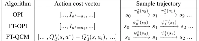
Figure 2: Training data generation and ranking reduction for each algorithm. Start by sampling
s0 from the same initial state distributionµ0. OPI uses the optimal policy at each depth
whereas FT-OPI and FT-QCM use the most recently learned complete policy (at depth
d−1). OPI and FT-OPI use 0-1 costs. Only FT-QCM uses the Q cost function, which turns out to be critical for good performance.
5. Related Work
While there is a large body of work on integrating learning and planning, we do not know of any work on learning partial policies for speeding up online MDP planning.
There are a number of efforts that study model-based reinforcement learning (RL) for large MDPs that utilize tree search methods for planning with the learned model. Examples include RL using FSSS (Walsh et al., 2010), Monte-Carlo AIXI (Veness et al., 2011), and TEXPLORE (Hester and Stone, 2013). However, these methods focus on model/simulator learning and do not attempt to learn to speedup tree search, which is the focus of our work.
Work on learning search control knowledge in deterministic planning and games is more related. One research direction has been on learning knowledge for STRIPS-style deterministic planners. Examples of this approach are learning heuristics and policies for guiding best-first search (Yoon et al., 2008) or state ranking functions (Xu et al., 2009). The problem of learning leaf evaluation heuristics has also been studied in the context of deterministic real-time heuristic search (Bulitko and Lee, 2006). As another example, evaluation functions for game tree search have been learned from the “principle variations” of deep searches (Veness et al., 2009). A related body of work involves iterative deepening heuristic search and its variants (Korf, 1985; Reinefeld and Marsland, 1994). Control knowledge is typically leveraged using heuristic scoring functions, transposition tables and principal variations. These methods often improve search by using memory-intensive control knowledge (e.g., hash tables) and incrementally expanding the search, but do not provide theoretical guarantees. Nevertheless, the idea of progressive widening and iterative deepening is extremely appealing and one that we intend to explore more in future work.
There have been a number of efforts for utilizing domain-specific knowledge in order to im-prove/speedup MCTS, many of which are covered in recent surveys (Browne et al., 2012; Gelly et al., 2012). The two main methods involve progressive bias and progressive widening. The core idea of progressive bias involves adding a quantityf(s, a)for guiding action selection during search.
f(s, a)may be hand-provided (Chaslot et al., 2007), or learned (Gelly and Silver, 2007; Sorg et al., 2011). Generally, there are a number of parameters that dictate how strongly f(s, a) influences search and how that influence decays as search progresses. In Sorg et al. (2011), control knowledge is learned via policy-gradient techniques in the form of a reward function and used to guide MCTS with the intention of better performance given a time budget. So far, however, the approach has not been analyzed formally and has not been demonstrated on large MDPs. Experiments in small MDPs have also not demonstrated improvement in terms of wall clock time over vanilla MCTS. The second method, progressive widening, is more popular in problems with large or continuous action spaces. The main idea here is to start the search with small action sets and introduce new actions as search progresses (Cou¨etoux et al., 2011a,b). For example, one may add a new action (sometimes called “unpruning”) when the number of visits to a state exceeds a heuristically chosen threshold. Although progressive widening is intuitively appealing and clearly required for anytime search in large action spaces, we were unable to find any existing method that leverages control knowledge or works in a principled manner.
Finally, MCTS methods often utilize hand-coded or learned rollout policies (sometimes called “default policies”) to improve anytime performance. A very well-known example is MoGo (Gelly et al., 2006). While this approach has shown promise in specific domains such as Go, where the policies can be highly engineered for efficiency, we have found that the large computational over-head of a learned rollout policy makes its usage hard to justify. The key issue is that the use of any learned rollout policy requires the evaluation of a feature vector at each state (or state-action pair) encountered during the rollout. Rollouts are typically far longer than the depth of the search tree, especially during the initial part of the sequential problem. This results in a massive number of additional feature evaluations, far greater than the number of evaluations performed by the heuristic bias methods discussed above which only require a feature evaluation once for every new action node added to the tree. Thus, the use of learned rollout policies may cause orders of magnitude fewer trajectories to be executed, compared to vanilla MCTS. In our experience, this can easily lead to degraded performance per unit time. Furthermore, there is little formal understanding about how to learn such rollout policies in principled ways, with straightforward approaches often yielding decreased performance (Silver and Tesauro, 2009).
6. Experiments
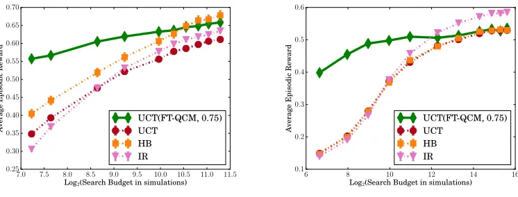
We perform a large-scale empirical evaluation of the partial policy learning algorithms on two chal-lenging MDP problems. The first, Galcon, is a variant of a popular real-time strategy game, while the second is Yahtzee, a classic dice game. Both problems pose a serious challenge to MCTS al-gorithms, for different reasons. However, in both domains, UCT, enhanced with learned partial policies, is able to significantly improve real-time search performance over every baseline. The key experimental findings are listed next.
2. UCT(FT-QCM) performs significantly better than vanilla UCT and other “informed” UCT variants when the search budget is small. Given a larger search budget, UCT(FT-QCM) wins in Galcon and achieves parity in Yahtzee.
3. The average regret of the pruning policies on a supervised dataset of states is strongly cor-related with the search performance, which is in line with our formal results. FT-QCM has significantly lower regret than FT-OPI and OPI.
4. The quality of the training data deteriorates quickly as depthdincreases. Regret increases as
dincreases.
5. It is critical to incorporate the computational cost of using control knowledge into the search budget during evaluation. Ignoring the computational cost of knowledge can significantly change the perceived relative performance of different algorithms.
6.1 Experimental Domains
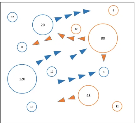
Galcon: The first domain is a variant of a popular two-player real-time strategy game, illustrated in Figure 3. The agent seeks to maximize its population by launching variable-sized population fleets from one of the planets currently under its control. The intention may be to either reinforce planets already controlled, attack an enemy planet, or capture an unclaimed planet. This produces a large action space (O |planets|2), where an action is defined as the triple (source planet, destination planet, fleet size). In our experiments, we use maps with 20 planets and three discrete levels of fleet size (small, medium, large). This often leads to game states where the action space contains hundreds of actions. The exact set of actions varies during the game as control over planets changes. State transitions are typically deterministic, unless a battle occurs. During each battle, a unit is randomly chosen from the two armies for termination. The battle ends when only one army remains. The maximum length of a game is restricted to 90 moves.
The search complexity caused by the large action branching factor is exacerbated by the rela-tively slow simulator and the length of the game. In this setting, UCT can only perform a small number of rollouts even when the search budget is as large as eight seconds per move. In fact, even at the largest search budgets, UCT only sparsely expands the tree beyond depths two or three. Note, however, that the rollout component of UCT is run to the end of the game and hence provides information well beyond these shallow depths. Finally, the second player or adversary is fixed to be a UCT agent with a budget of one second per move. All evaluations are performed against this fixed adversary. Note that at one second per decision, the fixed adversary effectively acts randomly, especially during the initial part of the game. However, further increase in the adversary’s search budget is impractical because of the significant computational cost of evaluating search agents in this domain.
Figure 3: A visualization of a Galcon game in progress. The agent must direct variable-sized fleets to either reinforce planets under its control, take over enemy planets, or unoccupied ones. The decision space is large, often involving hundreds of actions.
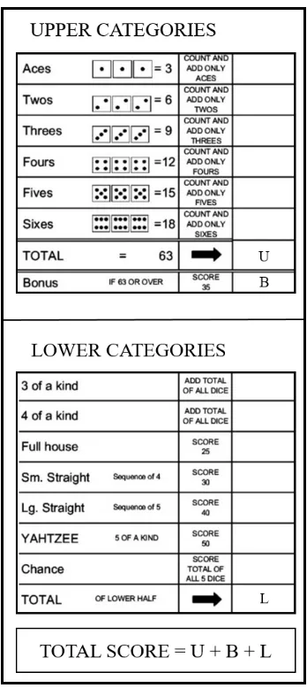
Yahtzee: The second domain is a classic dice game which consists of thirteen stages. In each stage, the agent may roll any subset of the five dice at most twice, after which the player must select one of the empty categories. A category, once selected, may not be reselected in later stages. This produces a total of 39decisions that must be made per game, where the last action trivially assigns the only remaining category. The categories are divided into upper and lower categories with each one scored differently. The lower categories roughly correspond to poker-style conditions (“full house”, “three of a kind”, “straight”, etc.), while the upper categories seek to maximize the individual dice faces (ones, twos, ..., sixes). A bonus of 35 points is awarded when the sum of the upper category scores exceeds 63. This ensures that the player must very carefully assign categories since the loss of the bonus has a large impact on the final score. The maximum score at the end of any game is 375, which is very hard to achieve. The above implementation is the simplest version of the game, restricted to a single “Yahtzee” (all five dice faces are identical). Our implementation for the simulator will be made available upon request4. Figure 4 shows a summary of the rules of the game. The UCT algorithm, including all parameter values, is identical to the one used in Galcon.
The trees generated by UCT differ significantly in the two domains. Compared to Galcon, Yahtzee has a relatively small action branching factor, smaller time horizon and a fast simulator. Furthermore, the available actions and the branching factor in Yahtzee decrease as categories are filled, whereas in Galcon, the agent occupying more planets has a larger action set. Thus, we can play many more games of Yahtzee per unit time compared to Galcon. However, Yahtzee poses a dif-ficult challenge for MCTS algorithms due to the dice rolls which increase the state branching factor and add variance to the Q value estimates. Consequently, even deep search with the UCT algorithm is error-prone and struggles to improve performance with larger search budgets. As in Galcon, the search quality of UCT degrades significantly at depths beyond two or three. Note, however, that
the performance degradation in Yahtzee is primarily caused by the transition stochasticity from the dice rolls, although the action branching factor remains significant. As in Galcon, UCT rolls out trajectories to the end of the game. Doing so provides information from states much deeper than the depth of the tree.
Normalizing rewards
The final score is always non-negative for Yahtzee, but may be negative for Galcon if the agent loses the game. In order to achieve a consistent comparison between the supervised metrics and search performance, we perform a linear rescaling of the score so that the performance measure now lies in the interval[0,1]. In our experiments, we provide this measure as reward to the agent at the end of each trajectory. That is, rewards are zero everywhere except in terminal state-action pairs. Note that a reward above0.5indicates a win in Galcon. In Yahtzee, a reward value of1.0is the theoretical upper limit achievable in the best possible outcome, which rarely occurs in practice. Furthermore, even a small increase in the reward (e.g.,0.1) is a significant improvement in Yahtzee.
6.2 Partial Policy Learning Setup
We now describe the procedure used to generate training data for the three learning algorithms, OPI, FT-OPI, and FT-QCM. Each algorithm is provided with root states generated by playing approxi-mately200full games. In Galcon, UCT is allowed to search for600seconds per move, whereas in Yahtzee, UCT is given120seconds per move. Each game results in a trajectory of states visited during the game. All of those states across all games constitute the set of root states used for train-ing as described in section 4. Despite the enormous search budget, depths beyond two or three are sparsely expanded, due to the large state and action branching factors. We therefore set the search depth bound (D) to3for learning, since the value estimates produced by UCT for deeper nodes are often inaccurate. Thus, the learned partial policy has the formψ= (ψ0, ψ1, ψ2). When UCT
gen-erates tree nodes at depths greater thanD, we prune usingψ2. As previously mentioned, we do not
limit the rollouts of UCT to depthD. Rather, the rollouts proceed until terminal states, which pro-vide a longer-term heuristic evaluation for tree nodes. However, we have confirmed experimentally that such nodes are not visited frequently enough for pruning to have a significant impact.
As previously mentioned, we learn partial policies by learning linear scoring functions. This requires us to compute state-action featuresφ(s, a)that capture salient attributes. We now describe the features used in each domain.
Yahtzee features: The features for the current state-action pair are defined over the next state, which is sampled by calling the simulator on the current state-action pair. The state-action feature vector is specified using a sparse one-hot encoding, where each of the 13 categories has 100 features assigned to it with one additional bias feature. The feature value for each unfilled category is a measure of how “close” the dice are to achieving the maximum score for that category, discretized into 100 bins. A perfect score returns a feature value of 1, whereas a category selection that does not add to the game score returns a feature value of 0. However, “select” actions for the upper categories that achieve binary outcomes (e.g., either a “full house” is achieved or not), are encoded using binary indicator features. All “roll” actions use discretized features, encoding how close the roll action brings the dice to a desired configuration. Note that there is large variance in the state-action features due to the dice rolls. This variance may be reduced by sampling more states and averaging. However, doing so would significantly increase the computational overhead of computingφ(s, a).
Evaluation metrics:We report the search budget in real-time (e.g.,4seconds per move) instead of the number of simulations. Each point on the anytime curve is the average of 1000 final game scores, with95%confidence intervals. This large-scale evaluation has massive computational cost and requires access to a cluster. The use of time-based search budgets in a cluster environment adds variance, requiring additional evaluations and averaging. However, an important result of the following experiments is that the use of time to measure budgets is essential for a fair comparison of “knowledge-injected” search algorithms.
6.3 Comparing OPI, FT-OPI, and FT-QCM
We learn ranking functions using each of the three learning algorithms, as described in section 4.2. We obtain a set of partial policies by varying the pruning thresholdsσd. Recall from section 4.2 that
our implementation of rank function learning does not depend onσd. The learned partial policies are
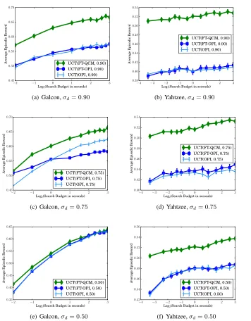
used to prune actions during search. Figure 5 shows the impact on search performance using UCT as the fixed base search algorithm. The first row shows the results for a large amount of pruning (σd= 0.90) while the second and third rows have progressively smaller pruning thresholds.
The first observation is that FT-QCM is clearly better than FT-OPI and OPI in both domains. FT-OPI and OPI are only competitive with FT-QCM in Galcon if small pruning is applied (bottom left). In Yahtzee, FT-QCM is significantly better even when the pruning is reduced to50%.
Second, we observe that all search algorithms perform better as the search budget is increased. However, the pruning thresholds significantly impact the performance gain across the anytime curve. In Galcon, this impact is highlighted by the steep curves forσd = 0.5, compared to the relatively
flat curves for larger pruning thresholds. In Yahtzee, although performance appears to increase very slowly, this small increase corresponds to a significant improvement in playing strength.
−2 −1 0 1 2 3 Log2(Search Budget in seconds)
0.45 0.50 0.55 0.60 0.65 0.70 A verage Episodic Rew ard UCT(FT-QCM, 0.90) UCT(FT-OPI, 0.90) UCT(OPI, 0.90)
(a) Galcon,σd= 0.90
−4 −3 −2 −1 0 1 2 3 Log2(Search Budget in seconds)
0.38 0.40 0.42 0.44 0.46 0.48 0.50 0.52 0.54 A verage Episodic Rew ard UCT(FT-QCM, 0.90) UCT(FT-OPI, 0.90) UCT(OPI, 0.90)
(b) Yahtzee,σd= 0.90
−2 −1 0 1 2 3
Log2(Search Budget in seconds) 0.45 0.50 0.55 0.60 0.65 0.70 A verage Episodic Rew ard UCT(FT-QCM, 0.75) UCT(FT-OPI, 0.75) UCT(OPI, 0.75)
(c) Galcon,σd= 0.75
−4 −3 −2 −1 0 1 2 3 Log2(Search Budget in seconds)
0.40 0.42 0.44 0.46 0.48 0.50 0.52 0.54 A verage Episodic Rew ard UCT(FT-QCM, 0.75) UCT(FT-OPI, 0.75) UCT(OPI, 0.75)
(d) Yahtzee,σd= 0.75
−2 −1 0 1 2 3
Log2(Search Budget in seconds) 0.35 0.40 0.45 0.50 0.55 0.60 0.65 A verage Episodic Rew ard UCT(FT-QCM, 0.50) UCT(FT-OPI, 0.50) UCT(OPI, 0.50)
(e) Galcon,σd= 0.50
−4 −3 −2 −1 0 1 2 3 Log2(Search Budget in seconds)
0.42 0.44 0.46 0.48 0.50 0.52 0.54 0.56 A verage Episodic Rew ard UCT(FT-QCM, 0.50) UCT(FT-OPI, 0.50) UCT(OPI, 0.50)
(f) Yahtzee,σd= 0.50
6.4 Relating search and regret
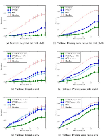
In order to better understand how search performance is related to the quality of the pruning policies, we analyze the learned partial policies on a held-out dataset of trajectories. In particular, for each linear partial policy, we compute its average pruning error and average regret as the level of pruning is increased from none (σd= 0) to maximum (σd= 1.0). Recall the definition of pruning error from
Equation 4, which is the probability ofψpruning away the optimal action (w.r.t. the expert policy). The definition for regret is given in Equation 3. These supervised metrics are computed by averaging over a held-out dataset of root states taken from at least one thousand trajectories. Figure 6 shows these supervised metrics on Galcon for each of the three depths. The left column shows the average regret while the right column is the average pruning error rate. The result of pruning randomly is also shown since it corresponds to pruning with random action subsets. Figure 7 shows the corresponding results for Yahtzee.
We start at the root, which is the first row in both figures. As expected, both regret and error increase as more actions are pruned. The key result here is that FT-QCM has significantly lower regret than FT-OPI and OPI for both domains. The lower regret is unsurprising given that FT-QCM uses the regret-based cost function while FT-OPI and OPI use zero-one costs. However, FT-QCM also demonstrates the least pruning error in both problems. Given that the same state distribution is used at the root, this observation merits additional analysis.
There are two main reasons why FT-OPI and OPI do not learn good policies. First, the linear policy space has very limited representational capacity. Second, the expert trajectories are noisy. The poor quality of the policy space is highlighted by the spike in the regret at maximum pruning, indicating that all three learners have difficulty imitating the expert. We also observe this at the end of training, where the final 0-1 error rate remains high. The expert’s shortcomings lie in the difficulty of the problems themselves. For instance, in Galcon, very few action nodes at depthsd >0receive sufficient visits. In Yahtzee, the stochasticity in dice rolls makes it very difficult to estimate action values accurately. Furthermore, in states where many actions are qualitatively similar (e.g., roll actions with nearly identical Q values), the expert’s choice of action is effectively random. This adds noise to the training examples, which makes the imitation learning problem harder. However, FT-QCM’s use of regret-based costs allows it to work well in Yahtzee at all depths, but only at the root in Galcon. In Galcon, the expert deteriorates rapidly away from the root policy and the training dataset becomes very noisy. Given the dominating performance of FT-QCM over OPI and FT-OPI, we focus on FT-QCM for the remainder of the experiments.
6.5 Selectingσd
We will now describe a simple technique for selectingσd. Recall that a good pruning threshold must
“pay for itself”. That is, in order to justify the time spent evaluating knowledge, a sufficient number of sub-optimal actions must be pruned so that the improvement produced is larger than what would have been achieved by simply searching more. At one extreme, too much pruning incurs large regret and little performance improvement with increasing search budgets. At the other extreme, if insufficient actions are pruned, search performance may be worse than that of uninformed (vanilla) search due to the additional overhead of computing state-action features.
The key to selecting good values lies in the supervised metrics discussed above, where the regret and search graphs are correlated. Thus, one simple technique for selectingσdis to use the largest
0.0 0.2 0.4 0.6 0.8 1.0 Pruning Ratio (σ)
0.000 0.005 0.010 0.015 0.020 0.025 Regret( µ0 ) FT-QCM FT-OPI OPI Random
(a) Galcon: Regret at the root (d=0)
0.0 0.2 0.4 0.6 0.8 1.0
Pruning Ratio (σ) 0.0 0.2 0.4 0.6 0.8 1.0 Pr( er ror ) FT-QCM FT-OPI OPI Random
(b) Galcon: Pruning error rate at the root (d=0)
0.0 0.2 0.4 0.6 0.8 1.0
Pruning Ratio (σ) 0.000 0.005 0.010 0.015 0.020 0.025 Regret( µ0 )
FT-QCM,σ0= 0.75
FT-OPI,σ0= 0.75
OPI Random
(c) Galcon: Regret at d=1
0.0 0.2 0.4 0.6 0.8 1.0
Pruning Ratio (σ) 0.0 0.2 0.4 0.6 0.8 1.0 Pr( er ror )
FT-QCM,σ0= 0.75
FT-OPI,σ0= 0.75
OPI Random
(d) Galcon: Pruning error rate at d=1
0.0 0.2 0.4 0.6 0.8 1.0
Pruning Ratio (σ) 0.000 0.005 0.010 0.015 0.020 0.025 Regret( µ0 )
FT-QCM,σ0,1= 0.75
FT-OPI,σ0,1= 0.75
OPI Random
(e) Galcon: Regret at d=2
0.0 0.2 0.4 0.6 0.8 1.0
Pruning Ratio (σ) 0.0 0.2 0.4 0.6 0.8 1.0 Pr( er ror )
FT-QCM,σ0,1= 0.75
FT-OPI,σ0,1= 0.75
OPI Random
(f) Galcon: Pruning error rate at d=2
Figure 6: Average regret and pruning error for the learned partial policiesψdas a function of the
pruning ratio in Galcon. The metrics are evaluated with respect to a held-out test set of states obtained from at least 1000 trajectories with root states sampled fromµ0. FT-QCM