Numerical Simulation by Galerkin Method
of 2D Nonlinear Convection-Diffusion
Cláudia Narumi Takayama Mori1 , Estaner Claro Romão1
1
Department of Basic and Environmental Sciences, Engineering School of Lorena, University of
São Paulo, Brazil
Abstract: The objective of this paper is to numerically solve a 2D Transient Nonlinear Convection-Diffusion Equation using the Galerkin Method. For numerical formulation, the Crank-Nicolson Method was used for temporal discretization, the Newton Method for linearization of the nonlinear terms, the Galerkin Method for spatial discretization and the Finite Differences Method for calculating the derivatives. Finally, to analyze the results obtained in the applications presented in this work the L norm was used from the comparison
with exact solutions.
Keywords: Nonlinear Convection-Diffusion, Galerkin Method, Newton Method, Numerical Simulation.
1. Introduction – Model Equation
In this work we intend to solve numerically the problem of 2D transient nonlinear
convection-diffusion governed by the equation,
𝜕𝑢 𝜕𝑡+ 𝑢
𝜕𝑢 𝜕𝑥+ 𝑢
𝜕𝑢 𝜕𝑦= 𝑣
𝜕2𝑢
𝜕𝑥2+ 𝑣
𝜕2𝑢
𝜕𝑦2 (1)
where 𝑢 is velocity component in x direction, 𝑣 is the cinematic viscosity (m²/s). The Equation (1) it is a simplification for only one variable of the 2D Burgers Equation [1-3].
2. Formulation
The following will be presented the methodological sequence for the formulation of the
problem governed by Equation (1).
2.1 Temporal Discretization
For temporal discretization, the traditional Cranck-Nicolson method [4] will be used in
𝑢𝑛 +1− 𝑢𝑛
∆𝑡 ≅ 1 2 𝑣
𝜕2𝑢𝑛+1
𝜕𝑥2 + 𝑣
𝜕2𝑢𝑛 +1
𝜕𝑦2 − 𝑢𝑛+1
𝜕𝑢𝑛 +1
𝜕𝑥 − 𝑢𝑛 +1 𝜕𝑢𝑛 +1
𝜕𝑦
+1 2 𝑣
𝜕2𝑢𝑛
𝜕𝑥2 + 𝑣
𝜕2𝑢𝑛
𝜕𝑦2 − 𝑢𝑛
𝜕𝑢𝑛
𝜕𝑥 − 𝑢𝑛 𝜕𝑢𝑛
𝜕𝑦 (2)
2.2 Linearization – Newton Method
Note in Equation (2), in the current step of time n + 1, two non-linear terms. To
linearize such terms will be used Newton's Method [5-7] that from the reasoning of the
expression,
𝑢𝑛+1𝜕𝑢𝑛 +1
𝜕𝑥 ≅ 𝑢𝑛 +1 𝜕𝑢𝑛
𝜕𝑥 + 𝑢𝑛 𝜕𝑢𝑛 +1
𝜕𝑥 − 𝑢𝑛 𝜕𝑢𝑛
𝜕𝑥 (3)
that when substituted in Equation (2) is obtained,
𝑢𝑛 +1− 𝑢𝑛
∆𝑡 = 1 2 𝑣
𝜕2𝑢𝑛+1
𝜕𝑥2 + 𝑣
𝜕2𝑢𝑛 +1
𝜕𝑦2 − 𝑢𝑛+1
𝜕𝑢𝑛
𝜕𝑥 − 𝑢𝑛 𝜕𝑢𝑛 +1
𝜕𝑥 − 𝑢𝑛 +1 𝜕𝑢𝑛
𝜕𝑦 − 𝑢𝑛 𝜕𝑢𝑛 +1
𝜕𝑦
+1 2 𝑣
𝜕2𝑢𝑛
𝜕𝑥2 + 𝑣
𝜕2𝑢𝑛
𝜕𝑦2 (4)
2.3 Spatial Discretization – Galerkin Method
For spatial discretization of Equation (4) the Galerkin Method [8] will be used by the
expression,
𝑅𝑊𝑑𝛺
𝛺
= 0 (5)
where W is adopted as the interpolation functions and R is the residual equation. In other words, applying Equation (5) in the result obtained in Equation (4), we obtain,
𝑢𝑛 +1
∆𝑡
Ω
𝑁𝑖𝑑Ω+1
2 −𝑣
𝜕2𝑢𝑛 +1
𝜕𝑥2 − 𝑣
𝜕2𝑢𝑛+1
𝜕𝑦2 + 𝑢𝑛 +1
𝜕𝑢𝑛
𝜕𝑥 + 𝑢𝑛 𝜕𝑢𝑛+1
𝜕𝑥 + 𝑢𝑛 +1 𝜕𝑢𝑛
𝜕𝑦
Ω
+ 𝑢𝑛𝜕𝑢𝑛+1
𝜕𝑦 𝑁𝑖𝑑Ω= 𝑢𝑛
∆𝑡
Ω
𝑁𝑖𝑑Ω+1 2 𝑣
𝜕2𝑢𝑛
𝜕𝑥2 + 𝑣
𝜕2𝑢𝑛
𝜕𝑦2
Ω
Using the principle of part integration of Differential and Integral Calculus, the
second-order terms of Equation (6) can be simplified as follows,
𝑣𝜕𝑥𝜕 𝜕𝑢𝜕𝑥
Ω
𝑁𝑖𝑑Ω= 𝑣𝜕𝑢 𝜕𝑥
𝛤
𝑁𝑖cos 𝜃 𝑑𝛤 − 𝑣𝜕𝑁𝑖 𝜕𝑥
𝜕𝑢 𝜕𝑥
Ω
𝑑Ω (7)
𝑣 𝜕 𝜕𝑦
𝜕𝑢 𝜕𝑦
Ω
𝑁𝑖𝑑Ω= 𝑣
𝜕𝑢 𝜕𝑦
𝛤
𝑁𝑖sen 𝜃 𝑑𝛤 − 𝑣
𝜕𝑁𝑖 𝜕𝑦
𝜕𝑢 𝜕𝑦
Ω
𝑑Ω (8)
In addition to replacing the results presented in Equations (7-8) in Equation (6) we also
replace the approximation
𝑢 ≅ 𝑢𝑒 = 𝑁
𝑗 𝑥, 𝑦 𝑢𝑗𝑒 𝑁𝑛𝑜𝑑𝑒𝑠
𝑗 =1
(9)
(where Nnodes is number of nodes in element)results in,
1 ∆𝑡+
1 2
𝜕𝑢𝑗𝑛 ,𝑒 𝜕𝑥 +
1 2
𝜕𝑢𝑗𝑛,𝑒 𝜕𝑦 𝑁𝑖
Ω𝑒
𝑁𝑗𝑑Ω𝑢𝑗𝑛+1,𝑒+𝑣 2
𝜕𝑁𝑖 𝜕𝑥
𝜕𝑁𝑗
𝜕𝑥 𝑑Ω𝑢𝑗𝑛 +1,𝑒
Ω𝑒 +𝑣 2 𝜕𝑁𝑖 𝜕𝑦 𝜕𝑁𝑗
𝜕𝑦 𝑑Ω𝑢𝑗𝑛+1,𝑒+
Ω𝑒
𝑢𝑗𝑛 ,𝑒 2 𝑁𝑖
Ω𝑒
𝜕𝑁𝑗
𝜕𝑥 𝑑Ω𝑢𝑗𝑛 +1,𝑒
+𝑢𝑗
𝑛 ,𝑒
2 𝑁𝑖
Ω𝑒
𝜕𝑁𝑗
𝜕𝑦 𝑑Ω𝑢𝑗𝑛 +1,𝑒
= 1 ∆𝑡 𝑁𝑖
Ω𝑒
𝑁𝑗𝑑Ω𝑢𝑗𝑛 ,𝑒−𝑣 2
𝜕𝑁𝑖 𝜕𝑥
𝜕𝑁𝑗
𝜕𝑥 𝑑Ω𝑢𝑗𝑛 ,𝑒
Ω𝑒 −𝑣 2 𝜕𝑁𝑖 𝜕𝑦 𝜕𝑁𝑗
𝜕𝑦 𝑑Ω𝑢𝑗𝑛,𝑒 +
Ω𝑒 +𝑣 2 𝜕𝑢𝑛 𝜕𝑥 𝛤
𝑁𝑖cos 𝜃 𝑑𝛤 +
𝑣 2
𝜕𝑢𝑛
𝜕𝑦
𝛤
𝑁𝑖sen 𝜃 𝑑𝛤 +
𝑣 2
𝜕𝑢𝑛 +1
𝜕𝑥
𝛤
𝑁𝑖cos 𝜃 𝑑𝛤
+𝑣 2
𝜕𝑢𝑛 +1
𝜕𝑦
𝛤
𝑁𝑖sen 𝜃 𝑑𝛤 (10)
In the form of matrix system,
𝐾 𝑢𝑗𝑛+1,𝑒 = 𝐹 − 𝐻 𝑢
𝑗𝑛 ,𝑒 (11)
𝐾𝑖𝑗 =
1 ∆𝑡+
1 2
𝜕𝑢𝑗𝑛,𝑒 𝜕𝑥 +
1 2
𝜕𝑢𝑗𝑛 ,𝑒 𝜕𝑦 𝑁𝑖
Ω𝑒
𝑁𝑗𝑑Ω+
𝑣 2
𝜕𝑁𝑖 𝜕𝑥
𝜕𝑁𝑗 𝜕𝑥 𝑑Ω
Ω𝑒 +𝑣 2 𝜕𝑁𝑖 𝜕𝑦 𝜕𝑁𝑗 𝜕𝑦 𝑑Ω
Ω𝑒
+𝑢𝑗
𝑛 ,𝑒
2 𝑁𝑖
Ω𝑒
𝜕𝑁𝑗 𝜕𝑥 𝑑Ω+
𝑢𝑗𝑛 ,𝑒 2 𝑁𝑖
Ω𝑒
𝜕𝑁𝑗
𝜕𝑦 𝑑Ω (12)
𝐻𝑖𝑗 = −
1 ∆𝑡 𝑁𝑖
Ω𝑒
𝑁𝑗𝑑Ω+
𝑣 2
𝜕𝑁𝑖 𝜕𝑥
𝜕𝑁𝑗 𝜕𝑥 𝑑Ω
Ω𝑒 +𝑣 2 𝜕𝑁𝑖 𝜕𝑦 𝜕𝑁𝑗 𝜕𝑦 𝑑Ω
Ω𝑒
(13)
𝐹𝑖 =
𝑣 2
𝜕𝑢𝑛
𝜕𝑥
𝛤
𝑁𝑖cos 𝜃 𝑑𝛤 +
𝑣 2
𝜕𝑢𝑛
𝜕𝑦
𝛤
𝑁𝑖sen 𝜃 𝑑𝛤 +
𝑣 2
𝜕𝑢𝑛 +1
𝜕𝑥
𝛤
𝑁𝑖cos 𝜃 𝑑𝛤
+𝑣 2
𝜕𝑢𝑛+1
𝜕𝑦
𝛤
𝑁𝑖sen 𝜃 𝑑𝛤 (14)
4. Numerical Applications
To analyze the efficiency of the proposed numerical formulation two applications with
exact solutions to perform the comparison are presented. From the solution of the linear system
in (11), through a computer code constructed via Fortran Language the numerical results will be
presented next. It is important to note that for the construction of the linear system in (11),
knowing that this is highly sparse, it used a technique proposed by [9] where three vectors are
constructed assuming only the nonzero coefficients of matrix K of system (11). Thus, from
these three vectors we construct two integers vectors (one containing the row position and the
other the column position of each non-zero coefficient) and a "ordered" real vector of nonzero
coefficients. Further details of the advantages of constructing the system in this way can be
found in [9]. To analyze the numerical efficiency of the proposed formulation will be used the
L norm that presents the larger absolute error committed in the computer domain.
4.1 First Application
In this first application, it was adopted as spatial domain a square of side 0.1 (L = 0.1) and a total time of 0.1 (Lt = 0.1). The viscosity was varied at values 1, 5 and 10, and the spatial
(Δx = Δy) and temporal (Δt) meshes were varied according to Tables 1 to 3. The spatial mesh was constructed from quadrilateral elements with four nodes and the interpolation functions
used can be found in [10]. For analysis of the error was used as exact solution the expression,
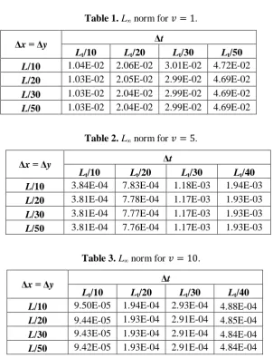
Table 1.L norm for 𝑣 = 1.
Δx = Δy Δt
Lt/10 Lt/20 Lt/30 Lt/50
L/10 1.04E-02 2.06E-02 3.01E-02 4.72E-02 L/20 1.03E-02 2.05E-02 2.99E-02 4.69E-02 L/30 1.03E-02 2.04E-02 2.99E-02 4.69E-02 L/50 1.03E-02 2.04E-02 2.99E-02 4.69E-02
Table 2.L norm for 𝑣 = 5.
Δx = Δy Δt
Lt/10 Lt/20 Lt/30 Lt/40
L/10 3.84E-04 7.83E-04 1.18E-03 1.94E-03 L/20 3.81E-04 7.78E-04 1.17E-03 1.93E-03 L/30 3.81E-04 7.77E-04 1.17E-03 1.93E-03 L/50 3.81E-04 7.76E-04 1.17E-03 1.93E-03
Table 3.L norm for 𝑣 = 10.
Δx = Δy Δt
Lt/10 Lt/20 Lt/30 Lt/40
L/10 9.50E-05 1.94E-04 2.93E-04 4.88E-04 L/20 9.44E-05 1.93E-04 2.91E-04 4.85E-04 L/30 9.43E-05 1.93E-04 2.91E-04 4.84E-04 L/50 9.42E-05 1.93E-04 2.91E-04 4.84E-04
From the results presented in Tables 1 to 3 it can be noted that for the spatial
refinements adopted, the numerical results are already stagnant, while with the increase in
refinement in time, the numerical results decrease accuracy. Next, another application will be
presented to assess whether these situations recur.
4.2 Second Application
For this application will only be modified the exact solution proposed that in this case is
given by the expression,
𝑢 𝑥, 𝑦, 𝑡 = 1 1 + 𝑒𝑥+𝑦−𝑡2𝑣
After some numerical tests it was noticed that the behavior of the numerical solution for
this case was similar to that presented in application 1, that is, the greater the number of time
computational behavior of the first order derivatives of u did not show the same numerical efficiency as the numerical solution of u, as can be seen in Tables 4 and 5.
Table 4. L norm for 𝑣 = 1, x = y = L/20, t = Lt/10.
Time
steps L norm - u L norm - u/x
1 7.28E-05 1.83E-02
2 3.63E-06 1.73E-02
3 8.60E-05 1.64E-02
4 1.71E-04 1.54E-02
5 2.56E-04 1.44E-02
6 3.43E-04 1.38E-02
7 4.29E-04 1.73E-02
8 5.16E-04 2.08E-02
9 6.03E-04 2.43E-02
10 6.89E-04 2.78E-02
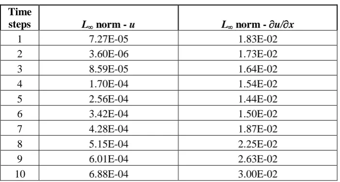
Note in the first term on the right side of Equation (12) that there is a need to calculate
the derivative of u, 𝜕𝑢𝑗
𝑛 ,𝑒
𝜕𝑥 and 𝜕𝑢𝑗𝑛 ,𝑒
𝜕𝑦 , that for the calculations performed and presented in Tables 4
and 5 the Finite Difference Method (Central Difference Method of order 2) was used. After that,
we used finite difference expressions of order 4, and the numerical results in the calculation of
the first derivative did not evolve.
It is important to note that the numerical results of u are good, however, the need to find an alternative to improve the first derivative calculation is clear.
Table 5. L norm for 𝑣 = 1, x = y = L/40, t = Lt/10.
Time
steps L norm - u L norm - u/x
1 7.27E-05 1.83E-02
2 3.60E-06 1.73E-02
3 8.59E-05 1.64E-02
4 1.70E-04 1.54E-02
5 2.56E-04 1.44E-02
6 3.42E-04 1.50E-02
7 4.28E-04 1.87E-02
8 5.15E-04 2.25E-02
9 6.01E-04 2.63E-02
5. Conclusion
The numerical results presented by the use of the Galerkin Method have proved to be
efficient, however, it is noted that the calculation of derivatives the u at each time step should be improved. For this, a first proposal for future work is to use quadrilateral elements with nine
nodes (quadratic elements) and to calculate the derivatives using finite element approximation.
Acknowledgements
The FAPESP (Procs. 2014/06679-8 and 2016/00928-1) supported the present work.
References
[1] Campos, M. D.; Romão, E. C.. A High-Order Finite-Difference Scheme with a Linearization Technique for Solving of Three-Dimensional Burgers Equation. Computer Modeling in Engineering & Sciences (Print), v. 103, p. 139-154, 2014.
[2] Srivastava, V. K.; Tamsir, M.; Bhardwaj, U.; Sanyasiraju, Y. V. S. S.. Crank-Nicolson Scheme for Numerical Solutions of Two-dimensional Coupled Burgers’ Equations. Int. J. Sci. & Eng. Research, vol. 2, no. 5, pp. 1-7, 2011.
[3] Bahadir, A. R.. A fully implicit finite-difference scheme for two dimensional Burgers equations. Appl. Math. Comput., vol. 137, pp. 131-137, 2003.
[4] Smith, G. D.. Numerical solution of partial differential equations: finite difference method, third ed., Clarendon Press, 1998.
[5] Campos, M. D.; Romão, E. C.; Moura, L. F. M.. A Finite-Difference Method of High-Order Accuracy for the Solution of Transient Nonlinear Diffusive Convective Problem in Three Dimensions. Case Studies Thermal Eng., vol. 3, pp. 43-50, 2014.
[6] Campos, M. D.; Romão, E. C.; Moura, L. F. M.. Linearization Technique and its Application to Numerical Solution of Bidimensional Nonlinear Convection Diffusion, Equation. Appl. Math. Sci., vol. 8, n. 15, pp. 743-750, 2014.
[7] Deblois, B. M.. Linearizing convection terms in the Navier-Stokes equations. Comp. Meth. Appl. Mech. Eng., vol. 143, no. 3-4, pp. 289-297, 1997.
[8] Reddy, J. N.. An introduction to the finite element method, 3ª Edition, McGraw-Hill, 2013.
[9] Romão, E. C.. Efficient Alternative for Construction of the Linear System Stemming from Numerical Solution of Heat Transfer Problems via FEM. Mathematical Problems in Engineering (Print), v. 2016, p. 1-7, 2016.