https://dx.doi.org/10.22075/IJNAA.2020.4206
Efficiency of Target Location Scenarios in the
Multi-Transmitter Multi-Receiver Passive Radar
S. Fooladi Talaria,∗, Dr. K. Mohamedpoura
aElectrical Engineering Department K.N.Toosi University of Technology, Tehran, Iran
(Communicated by M.B. Ghaemi)
Abstract
Multi-transmitter multi-receiver passive radar, which locates target in the surveillance area by the reflected signals of the available opportunistic transmitter from the target, is of interest in many applications. In this paper, we investigate different signal processing scenarios in multi-transmitter multi-receiver passive radar. These scenarios include decentralized processing of reference and lance signals, decentralized processing of surveillance signals, and centralized processing of surveil-lance signals that have different advantages, disadvantages, and requirements. A variety of possible measurements including TDOA, GROA, AOA and their combinations are presented under different scenarios. The Cramer Rao lower band (CRLB) is presented for different signal processing scenarios for the error of the target localization. The efficiency of the target localization for different signal processing scenarios and types of measurements has been investigated by the CRLB. As shown in the simulation results, the combined use of the measurements is always better than their single use. Also centralized and decentralized processing of surveillance signals, by arranging the receiver sensors in the far distances, can have better efficiency than close distance arrangements.
Keywords: Passive Radar, Multi-Transmitter Multi-Receiver Radar, Target Localization, Centralized Signal Processing, Decentralized Signal Processing.
2010 MSC: 68N30
1. Introduction
Passive radar locates the target by receiving reflected signals from the target in the several receiver sensors. These signals are radiated by the transmitters existing in the environment called
∗Corresponding Author
Email addresses: [email protected] (S. Fooladi Talari ), [email protected] (Dr. K. Mohamedpour )
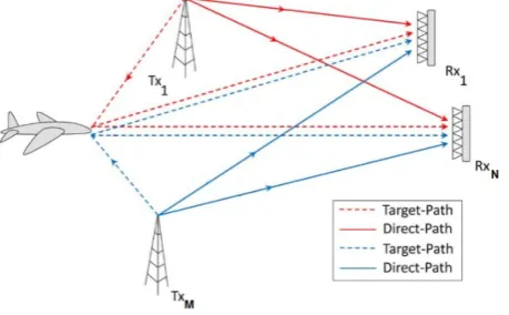
Figure 1: Geographic scheme of transmitters, receiver sensors, and target.
opportunistic transmitters. These radars for many years because of the features such as their latency in the magnetic spectrum, the low cost as compared to active radars, as well as no need of frequency allocation, have attracted much attention in various industries [1], [2], [3], [4], [5], [6], [7], [8], [9], [10]. latency in the frequency spectrum is due to the lack of signal radiation, cheapness as well as lack of need for frequency allocation due to not need on the transmitter. Various opportunistic transmitters, such as terrestrial broadcast transmitters including Radio FM, Digital Radio (DAB), Digital TV like DVB-T and DVB-T2 [11] have been investigated for use in the passive radar. On the other hand, various cellular telecommunication networks such as GSM [12], 3G and 4G [13] as well as Wi-Fi signals [14] and even satellite transmitters [15] such as GNSS [16] have also been investigated for this application [17], [18].
Target localization has been investigated under different scenarios such as active radars [19], [20]. Signal processing of passive radar is usually accomplished as multi-static active radars. Multi-static radar is created by the development of biMulti-static radars. In biMulti-static signal processing, it is necessary to receive the direct signal of the transmitter and the target reflection simultaneously. Target localization is done by extending or generalizing the bistatic radar to the multi-static radar [21], [22], [23]. Some processing scenarios and detection are reviewed by Hak [24], [25].
Localization of illuminator is studied in the context of passive source localization (PSL) [26], [27]. The effect of geographical topology has been investigated on PSL [28] that is similar to the centralized processing of reflected signals on the passive radar.
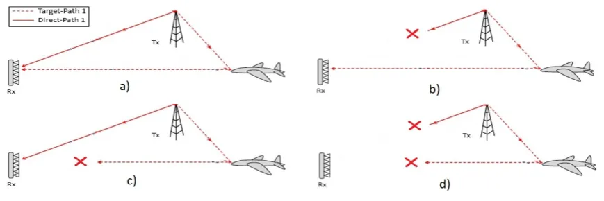
Figure 2: Different scenarios of receiving reference signals and surveillance signals
2. System model
Passive radar uses opportunistic transmitters in the environment. The target reflected signal is received by the receiver sensors in the passive radar. The geographical scheme of the problem is illustrated in Fig. 1. As shown, the M opportunistic transmitters radiate signals in the environment. The reflected signals from the target are received by the N receiver sensors. The receiver sensors use two separate channels to receive the direct path signal of the transmitter and the target reflection. Direct path signals are received from the reference channel while the reflected signals from the surveillance channel. The reference channel uses the directional antenna to receive the direct signal of the transmitter whereas the surveillance channel uses an array of omnidirectional antennas to receive the reflections.
2.1. Bistatic Scenario
The multi-transmitter multi-receiver passive radar system model, such as the MIMO radar is considered with the separated antennas. In the passive radar scenario, the transmitter is not under control of radar designers, and the transmitters are usually placed at large distances with each other to cover the under service area. However, the receiver sensors can be located at close distances. Passive radar processing is based on bistatic radar processing. Each pair of the bistatic signal consists of two signals of the transmitter and the target reflection. In the passive radar, several scenarios may occur for each pair of bistatic signals as shown in Fig. 2. These scenarios are developed by assuming the receiving or not receiving each of the direct path signals and/or the reflection and include:
a) Receive both direct signal and reflection in the receiver. b) Receive only the reflection signal.
c) Receive only direct signal. d) Receive none of the signals.
ssT xi,T a,Rxj(t) =
1 gT xi,T a,Rxj
sT xi(t−τT xi,T a,Rxj)a(θT a,Rxj, ϕT a,Rxj) (2.1)
srT xi,Rxj(t) =
1 gT xi,Rxj
τT xi,Rxj =
rT xi,Rxj
c (2.3) τT xi,T a,Rxj =
rT xi,T a+rT a,Rxj
c (2.4)
gT xi,Rxj =
(rT xi,Rxj)
γ
AT xi,RxjARxj,T xi
𝟋(2.5) gT xi,T a,Rxj =
(rT xi,T arT a,Rxj)
γ
AT xi,T a √σ
T xi,T a,RxjARxj,T a
𝟋(2.6)
θT xi,Rxj =arctan(
yT a−yRxj xT a−xRxj
)(2.7) ϕT a,Rxj =arcsin(
zT a−zRxj
rT a,Rxj
)(2.8)
The above modes are different for each pair of bistatic signals per receiver, depending on the pro-cessing scenario, the transmitters and receiver sensors arrangement, the target location and the area geography.
2.2. Signal model
Locations of transmitters are shownp
T xi = [xT xi yT xi zT xi]
T
by and Locations of receiver sensors are shown by p
Rxj = [xRxj yRxj zRxj]
T
. Where, i and j are the transmitter index and the receiver index, respectively. The target is located atp
T a = [xT a yT a zT a] T
. The reflected signal of transmitter i received by sensor j from the target which is presented in equation (2.1) and the received direct signal of transmitter i is presented in equation (2.2).
In these equations, srT xi,Rxj(t) is the received reference signal,ssT xi,T a,Rxj(t) is reflected signal
re-ceived from the target,sT xi(t) is transmitted signal of transmitter i, τ showe the path delay, g
depicts the path attenuation, θT a,Rxj and ϕT a,Rxj are the direction of arrival of the received signal in
receiverj. a(θT a,Rxj, ϕT a,Rxj)is the signal angular function of the reflection received from the target
at the receiver location. The values of these parameters depending on the characteristics of the target, transmitter, and receiver sensor are given in equations (2.3) to (2.8).
In equation (5) and (6), the Ax,y is gain of x’s antenna in the y direction,σT xi,T a,Rxj is the target RCS
value in bistatic angle of transmitter i, target, and receiverj,rx,y=||px−py|| is distance betweenpx
and p
y,c is the signal propagation speed, γ is the path loss component which usually considered
equal to 1, and 𝟋 denote other fixed parameters.||x|| shows the norm of vector x. It should be noted that by point target assumption that is true for the far-field target, the value of σT xi,T a,Rxj is
equal for all couples of receivers and transmitters and is denoted by σ. Assuming the transmitter and receiver locations are known, the direct signal will be independent of the angular function and a(θT a,Rxj, ϕT a,Rxj) can be considered equal to 1 in the equation. In fact, the receiver sensor by
directing the antenna to the transmitter receives the direct signals of the transmitter with maximum gain. Also assuming an omnidirectional antenna for the transmitter in the signal transmission, then the value ofAT xi, T ais independent of the target location and the value of AT xi,Rxj is independent of
the receiver location. Therefore, both parameters will be constant and equal to AT xi. Furthermore,
assuming an omnidirectional antenna for the receivers sensors, the parameter AT a,Rxj independent
of the target location will be equal toARxj.
2.3. Measurements model
reflected signal from the target are calculated. The target reflection signal is required for location processing. Therefore, two scenarios of receiving the reflection signal in the presence and absence of the direct transmitter signal are used for subsequent passive radar processing, including the target localization and tracking. Three types of reflection signals measurement can be performed that include TDOA, GROA, and AOA. The measurement vector is equal to:
k =τT gT θT ϕTT (2.9)
In the above equations ofk, τ, g, θ, and ϕ vectors are in the order of the vectors of all measure-ments, the TDOA, GROA, and DOA measurements respectively, azimuth angle and elevation angle of DOA measurements. The measurement of these vectors is associated with the noise that we model as additive noise. For the simplicity of calculations, we assume the measurement noises as additive Gaussian noise. Therefore, the measurement vector is equal to:
k =bk+nbk (2.10)
nbk ∼N(0, Q);diag(Q) =στ2T a2gT σ2θT σ2ϕTT (2.11) In the above equation,bk the vector represents the non-noise values of the measurements. σ2
τ,σ2g, σ2θ, andσ2ϕare the noise variance vectors of TDOA measurements, the noise of GROA measurement, noise of DOA measurement of azimuth angle and the noise of elevation angle measurements. Other scenarios of measurements are obtained by simplifying and reducing these vectors. These modes include alone TDOA, alone AOA, TDOA and AOA, TDOA and GROA, AOA and GROA.
3. Performance of target localization for different measurement scenarios
In the passive radar, the measurements accomplished by receiver sensors are dispatched to the central sensor for target locating and tracking. The central sensor engages in locating and tracking the target by per knowledge of locations of the receiver sensors and opportunistic transmitters and measurements taken at the receiver sensors. As mentioned, the available measurements include TDOA, GROA, and AOA. The measurement vector used for locating is shown in equation (2.10). All or some of these measurements can be used according to the scenario.
Measurements calculation on the passive radar by processing the received signals can be done cen-tralized on the central sensor or decencen-tralized on the receiver sensors. In the cencen-tralized processing scenario, the signals are dispatched to the central sensor and and part of signal processing is carried out there. In the decentralized processing scenario, signal processing is performed only on the receiver sensors and the measurements are sent to the central sensor. In the locating process, data association is a fundamental step. The data association involves specifying the opportunistic transmitter of the radiation’s received reflection on one hand and specifying the measurements done related to one tar-get in different receiver sensors on the other hand. This measurement allocation also depends on the type of opportunistic transmitters network topology. That is, after calculating the measurements, it must be determined which measurements belong to a specific target and which transmitter was the source of radiations. In some methods, this is done by considering all possible modes by MHT tracking algorithms [30].
τ =τT x1,T a,Rx1;T x1,Rx1 · · · τT x1,T a,RxN;T x1,RxN · · · τT xM,T a,Rx1;T xM,Rx1 · · · τT xM,T a,RxN;T xM,RxN
T
τT xi,T a,Rxj;T xi,Rxj =τT xi,T a,Rxj−τT xi,Rxj =
rT xi,T a,Rxj −rT xi,Rxj
c =
rT xi,T a+rT a,Rxj−rT xi,Rxj
c (3.2)
τ =τT a,Rx2;T a,Rx1|T x1 · · · τT a,RxN;T a,Rx1|T x1 · · · τT a,RxN;T a,RxN−1|T x1 · · · τT a,RxN;T a,RxN−1|T xM
T
(3.3)
τT a,Rxj;T xi,Rxl|T xi =τT a,Rxj −τT a,Rxl =
rT a,Rxj −rT a,Rxl
c (3.4)
τ =τT a,Rx2;T a,Rx1|T x1 · · · τT a,RxN;T a,Rx1|T x1 · · · τT a,Rx2;T a,Rx1|T xM · · · τT a,RxN;T a,Rx1|T xM
T
(3.5)
τT a,Rxj;T xi,Rx1|T xi =τT a,Rxj −τT a,Rx1 =
rT a,Rxj −rT a,Rx1
c (3.6)
g =gT a,Rx2;T a,Rx1|T x1 · · · gT a,RxN;T a,Rx1|T x1 · · · gT a,Rx2;T a,Rx1|T xM · · · gT a,RxN;T a,Rx1|T xM
T
(3.7)
gT a,Rxj;T xi,Rx1|T xi =
gT a,Rxj|T xi
gT a,Rx1|T xi
=
√σ
T xi,T a,Rx1ARx1,T arT a−Rxj √σ
T xi,T a,RxjARxj,T arT a−Rx1
(3.8)
θ =θT a,Rx1|T x1 · · · θT a,RxN|T x1 · · · θT a,Rx1|T xM · · · θT a,RxN|T xM
T
(3.9)
θT a,Rxj|T xi =atan(
(p
T a−pRxj)yT
(p
T a−pRxj)x
T);x=
1 0 0T ;y=0 1 0T (3.10)
ϕ =ϕT a,Rx1|T x1 · · · ϕT a,RxN|T x1 · · · ϕT a,Rx1|T xM · · · ϕT a,RxN|T xM
T
(3.11)
ϕT a,Rxj|T xi =asin(
(p
T a−pRxj)zT
rT a,Rxj
);z =0 0 1T (3.12)
3.1. Measurement vectors
This section presents measurement vectors under different processing scenarios. Considering two centralized and decentralized processing scenarios and two signal reception scenarios, reflections are provided in the presence or absence of a direct transmitter signal. We have three different scenarios for TDOA measurements: Decentralized processing of reference-surveillance channels, centralized processing of surveillance channels and decentralized processing of surveillance channels. In all cases, GROA and DOA measurements are calculated by the decentralized processing of surveillance channels. The total number of measurements for different scenarios is presented in Table 1.
3.1.1. TDOA measurements vector for decentralized processing of reference-surveillance channels
Both signals of the transmitter direct path and the target reflection are received in this scenario. The TDOA measurements are computed by decentralized processing of direct path signal received from the reference channel and the reflection signal received from the surveillance channel in the receiver sensors. In an MFN network, the number of M TDOA measurements can be calculated be-tween the reference and surveillance channels in each receiver sensor presented by the measurement vectors in equation (3.1). TDOAs can be obtained from cross ambiguity function of surveillance-reference channels. In the MFN network, there are M ×(N−1)measurements. In the SFN network, we haveN TDOA measurements that theT xi change to T xs in equation (3.1). Where,s indicates
the index of the strongest transmitter in that receiver. In these equations τT xi,T a,Rxj;T xi,Rxj is
pre-sented in equation (3.2).
3.1.2. TDOA measurements vector in centralized processing of surveillance channels
In this scenario, independent of whether or not to receive the direct path transmitter signal, all received reflections sampled at the receiving sensor must be transmitted to the central sensor. The TDOAs in the central sensor are calculated by processing the reflected signals received from the surveillance channels in the different receiver sensors relative to all other receiver sensors. TDOAs can be obtained from the cross ambiguity function of surveillance channels. In an MFN network, we have (N−1)/2 measurements for TDOA per each transmitter and compared to the surveillance channels of both receiver couples; the measurement vectors are presented in equation (3.3). In the SFN network, we have(N−1)/2number of TDOA measurements. In equation (3.3), the T xi changes
toT xs only. In these equations, τT a,Rxj,T a,Rxk|T xs is shown in equation (3.4).
3.1.3. TDOA measurements vector in decentralized processing of surveillance channels
In this scenario, independent of whether receiving or not receiving the direct path signal of the transmitters, received reflections are processed in the receiving sensors themselves. All receiver sensors must be synchronous with each other in clock and time reference. Signal processing is performed on each receiver sensor and calculated time of arrival (TOA) of reflection is transmitted to the central sensor. In the central sensor, the TDOA measurements are obtained from the difference of estimated TOA measurements of relations in the receiver sensors. To obtain TDOA, one has to use a specific pattern in the transmitter signal or a specific criterion in the receiver. In an MFN network, we have (N−1) number TDOA and GROA measurements per each transmitter. The measurement vectors are presented in equation (3.5). in the SFN network, we have (N−1) number TDOA measurements that the T xi change to T xs in equation (3.5). In these equations, τT a,Rxj,T a,Rx1|T xs is presented in equation (3.6).
3.1.4. GROA measurement vectors
in the receiver sensors by the estimated power in reference receiver sensor. In an MFN network, we have the N −1 number of measurements per transmitter. The measurement vectors are presented in equation (3.7). In the SFN network, we have 1 measurement in each receiver sensor against each strongest transmitter that the T xi change toT xs in this equation. Where, s indicates the index
of the strongest transmitter in that receiver. In this equation, gT a,Rxj;T xi,Rx1|T xi are presented in
equation (3.8).
3.1.5. DOA measurement vectors
Each receiver sensor can estimate the direction of the received reflection by the processing of received signals from the antenna array. In an MFN network, we have the N number of measurements per transmitter. The measurement vectors are presented in equations (3.9) and (3.10). In the SFN network, we have 1 measurement in each receiver sensor against each strongest transmitter that the T xi change to T xs in these equations. Where,s indicates the index of the strongest transmitter
in that receiver. In these equation, θT a,Rxj and ϕT a,Rxj are presented in equation (3.11) and (3.12),
respectively.
3.1.6. Rao Cramer Lower Band (CRLB)
This section presents a lower band of location estimation errors in multi-transmitter multi-receiver passive radar by TDOA, GROA, and AOA measurements. Assuming the noises of measurements are additive and Gaussian, the CRLB is obtained by using the Fisher Matrix to fit the used measurements and independent of the signal type. CRLB Matrix for p
T a is equal to [31]
CRLB=F IM−1(pT a) (3.13)
The FIM matrix represents the Fisher information matrix. Assuming the additive Gaussian noise assumption of measurement vectork FIM matrix is equal to
F IM(p T a= (
∂k ∂pT T a
)TQ−1( ∂k ∂pT T a
) (3.14)
∂k/∂pT
T a should be calculated for TDOA, GROA, and AOA measurements under centralized and
decentralized processing scenarios. This value for TDOA measurements with decentralized process-ing scenarios of surveillance-reference channels, centralized processprocess-ing of surveillance channels and decentralized processing of surveillance channels is presented in equations (3.15), (3.16), (3.17), and for GROA and AOA measurements by decentralized processing of surveillance, channel is presented in equations (3.18) and (3.19), respectively.
∂T xi,T a,Rxj;T xi,Rxj
∂pT T a
= 1 c(
[p
T a−pT xi] T
rT xi,T a
+ [p
T a−pRxj] T
rrxj,T a
) (3.15)
∂T a,Rxj;T a,Rxl
∂pT T a
= 1 c(
[p
T a−pRxj] T
rT a,Rxj
− [pT a−pRxl] T
rT a,Rxl
) (3.16)
∂gT a,Rxj;T a,Rxl
∂pT T a
= ARxl,T a
ARxj,T a
rσ
T xi,T a,Rxl
σT xi,T a,Rxj
rT a,Rxj
rT a,Rxl
( [p
T a−pRxj] T
r2
T a,Rxj
− [pT a−pRxl] T
r2
T a,Rxl
) (3.17)
∂θT a,Rxj
∂pT T a
= 1
l2
T a,Rxj
(([p
T a−pRxj]
Tx)y−[p
T a−pRxj]
∂gT a,Rxj;T a,Rxl
∂pT T a
= ARxl,T a
ARxj,T a
σT xi,T a,Rxl
σT xi,T a,Rxj
rT a,Rxj
rT a,Rxl
( [p
T a−pRxj] T
r2
T a,Rxj
− [pT a−pRxl] T
r2
T a,Rxl
) (3.19)
The matrix Q in equation (3.14) represents the covariance. The elements of this matrix are provided for the TDOA, GROA, and AOAdependent on the transmitted signal specifications and SNR value. On the other hand, the SNR of the received signal for the reflected signals. As obvious, the SNR is dependent on the range. Hence, regardless of the transmitter signal specification, the efficiency of locating through dependence on the variance of the measurements is dependent also on the inverse of square of range.
4. Simulation result
In this section, we present the simulation results of different processing scenarios. The Lower band of RMSE (Root Mean Square Error) of target location estimating will be provided with the square root of CRLB. The amount provided is of variable length and in meters. The simulations are presented in 3 different categories. The first section investigates the impact of the target location on the CRLB. In this case, the simulation results are shown with the colored contours, which indicate the RCRLB on the two-dimensional plane. These simulations provide an overview of the impact of the target location and the comparison of different scenarios. The second section investigates the impact of errors on different processing scenarios. In this case, the advantages and disadvantages of the scenarios will be observed for a variety of measurement errors. In the third cluster, the dependence of the accuracy of the measurement on the range is investigated. The locations of the transmitters are presented in Table (1). We consider the location of the receiver sensors under two categories of close distance and far distance sensors. Locations of receiver sensors in the close distance arrangement are presented in Table (2) and for the far distance arrangement is presented in Table (3).
4.1. Impact of the target location
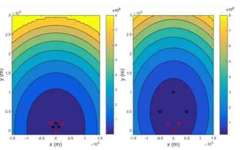
we Consider an area contains x and y equal to of AA and AA respectively in the Cartesian coordinates. The target altitude is considered equal to 9km in this area. We present the RCRLB value at different locations in this space. We also investigate several different arrangement scenarios. The sensors are assumed to use TDOA and azimuth angle of AOA measurements. The standard deviation of measurement errors for the time difference of arrival and direction of arrival are assumed equal to 100ns and 1deg respectively for different points of space. As shown in figures (3) to (6) for the different sensors arrangement of the receiver sensors. Centralized processing of surveillance chan-nels performs better than decentralized processing of surveillance chanchan-nels, but their performances are close together. processing of surveillance channels by far distance arrangement of receiver sen-sors has better performance than decentralized processing of reference-surveillance channels by close distance arrangement of receiver sensors. However, each of these processing scenarios has different requirements and limitations.
Table 1: Transmitters Table 2: Receivers sensors Table 3: Receivers sensors in close arrangement in the far arrangement
index x y z index x y z index x y z
1 0km 0km 100m 1 0 0 100m 1 0 0 100m
2 20km 20km 100m 2 10km 10km 200m 2 50km 50km 200m
3 -20km 20km 100m 3 -10km 10km 200m 3 -50km 50km 200m
Figure 3: RCRLB on plane x and y for TDOA and AOA azimuth angle measurements with standard deviations of measurements errors equal to 100ns and 1deg respectively, by one transmitter and 4 receivers at close range for a) decentralized processing of reference-surveillance channels, b) centralized processing of surveillance channels, and c) decentralized processing of surveillance channels.
Figure 4: RCRLB on plane x and y for TDOA and AOA azimuth angle measurements with standard deviations of measurements errors equal to 100ns and 1deg respectively, by 3 transmitters and 4 receivers at close range for a) decentralized processing of reference-surveillance channels, b) centralized processing of surveillance channels, and c) decentralized processing of surveillance channels.
4.1.1. A transmitter and close distance receiver sensors
In this scenario, the locations of receiver sensors are considered in accordance with Table (2) and only the first transmitter of the Table (1) is considered. The RCRLB value is shown for different locations in the area. Fig. 3 (a) shows the decentralized processing of the reference-surveillance channels. Figure b) shows the centralized processing of surveillance channels and figure c) shows the decentralized processing of surveillance channels. As shown, the RCRLB is limited to 20km. Decentralized processing of surveillance-reference channels has better efficiency than the other two methods. Furthermore, centralized processing of surveillance channels has better efficiency than the decentralized processing of them. however, this difference is low and performance is close together.
4.1.2. Three transmitters and close distance receiver sensors
surveil-lance channels, and figure c) shows the decentralized processing of surveilsurveil-lance channels. As shown, the RCRLB is limited to 10km. The use of decentralized processing of the reference-surveillance channel is better than the other two methods. The centralized processing of surveillance channels has better efficiency than the decentralized processing of them.
4.1.3. A transmitter and far distance receiver sensors
In this scenario, the locations of the receiver sensors are considered according to Table (3) and only the first transmitter of Table (1) is considered. The RCRLB value is shown for different locations of the area. Fig. 5 (a) shows centralized surveillance channels processing and figure b) shows decen-tralized processing of surveillance channels. The decendecen-tralized processing of reference-surveillance channels is not presented due to the impossibility of receiving the reference signal in this scenario. As shown, the RCRLB is limited to 10 km. The use of centralized processing of surveillance channels performs better than decentralized processing of surveillance channels, but their difference is low and the performances are close together. As it is obvious, the efficiency of centralized processing of surveillance channels by this far distance arrangement of receiver sensors is better than the decen-tralized processing of surveillance-reference channels by close distance arrangement of the receiver sensors.
4.1.4. Three transmitters and far distance receiver sensors
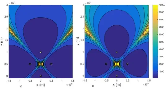
In this scenario, we consider the locations of the transmitters according to Table (1) and the receiver sensors according to Table (3). The transmitter network is considered as MFN and it is assumed that reflections caused by different transmitters’ radiations can be separated from each other in the receiver sensors. The RCRLB value is shown for different locations in the area. Fig. 6 a) shows the centralized processing of surveillance channels and figure b) shows the decentralized processing of surveillance channels. Decentralized processing of reference-surveillance channels is not provided like the previous scenario. As shown, the RCRLB is limited to 5km. The use of centralized processing of surveillance channels performs better than the decentralized processing of them, but their difference is low and the performances are close together. As it is obvious, the efficiency of centralized processing of surveillance channels by this far arrangement of receiver sensors is better than the decentralized processing of surveillance-reference channels by the close arrangement of receiver sensors.
Figure 6: RCRLB on plane x and y for TDOA and AOA azimuth angle measurements with standard deviations of measurements errors equal to 100ns and 1deg respectively, by 3 transmitters and 4 receivers at a remote distance for a) centralized processing of surveillance channels and b) decentralized processing of surveillance channels.
4.2. Effect of measurements errors
In this section, we present the impact of measurement errors on estimation efficiency by investi-gation of the lower band of error. The target is considered atp
T a= [40km 80km 9km] T
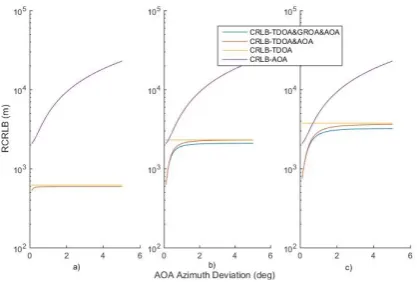
. We consider the transmitters of Table (1) and the arrangement of the receiver sensors as close distance in Table (2). Because of the far distance of the target to the transmitters and receiver sensors, we model it as point target and so it will be possible to use GROA measurements and its independence from the target RCS. Fig. 7 shows RCRLB vs standard division of TDOA error and Fig. 8 shows RCRLB vs the standard division of AOA error. The RCRLBs are shown for the scenarios of measurements include TDOA alone, AOA alone, TDOA and AOA combination and TDOA, GOA, and AOA com-bination in these figures. As illustrated, combined measurement mode has better efficiency than alone using of each measurement. As illustrated, CRLB of combined measurements is a function of measurement with a lower CRLB. where the CRLB of measurements is approximately equal, the Improvement caused by the combined use of measurements is more evident.
4.2.1. TDOA measurement error
Fig. 7 shows the RCRLB value vs standard deviation of the TDOA error from 10ns to 1us. The standard deviation of the azimuth angle and elevation angle of AOA measurement errors is 1deg and 5deg respectively. The standard deviation of GROA is considered equal to -15dB. Figure a) shows the decentralized processing efficiency of the reference-surveillance channels. Figures b) and c show the centralized processing of surveillance channels and the decentralized processing of them, respectively. As shown, the combined use of TDOA, GROA, and AOA measurements has better efficiency than other cases.
4.2.2. AOA measurement error
Figure 7: RCRLB vs TDOA standard deviation for a) decentralized processing of reference-surveillance channels, b) centralized processing of surveillance channels, and c) decentralized processing of surveillance channels.
Figure 8: RCRLB vs AOA azimuth angle standard deviation for a) decentralized processing of surveillance-reference channels, b) centralized processing of surveillance channels, and c) decentralized processing of surveillance channels.
4.2.3. Range dependency
To illustrate the dependence on range, we show the average effective range in the space. Figure 9 illustrates the mean of r2
T a,Rxj for and receivers, r
2
T xi,T ar
2
T a,Rxj don’t depend on receiver sensors
arrangement. The receiver sensors are according to Table (2) in Figure 9 a) and are according to Table (3) in Figure 9 b). As illustrated, the Value is limited to 89. The use of far distance arrangement of receiver sensors decreases effective range parameters. Thus, the SNR and accuracy of measurements improve.
5. Conclusion
Figure 9: Mean of Effective Range on plane x and y for a) receiver sensors of Table (2) and b) receiver sensors of Table (3).
the surveillance signals at the receiving sensors. The decentralized processing scenario of reference-surveillance signals requires the simultaneous reception of the direct signal of the transmitter and the target reflections. In centralized processing of surveillance signals, sampled signals at the re-ceiver sensors must be dispatched to the central sensor. In the decentralized processing scenario, the receiver sensors’ surveillance signals must be sampled synchronously in terms of time. The low band of estimation error is presented as a criterion for evaluating these passive radar localization scenarios. The proposed CRLB is provided for all scenarios and types of measurements used for target localization including TDOA and/or GROA and/or AOA. As shown in the simulation results, different combinations of measurements always lead to better accuracy than single use of them. Also, given the different scenarios of receiver sensor arrangement, centralized and decentralized processing of surveillance signals with receiver sensors arrangement at a far distance outperform close arrange-ment scenarios. The proposed method can also be used to select the optimal arrangearrange-ment for a given area and the known network of transmitters.
References
[1] N. Willis, H. D. Griffiths, Advances in Bistatic Radar, Scitech Pub Inc., (2007).
[2] H. D. Griffiths, C. J. Baker, An Introduction to Passive Radar, Artech House, (2017) . [3] M. Cherniakov, Bistatic Radar: Emerging Technology, JohnWiley Sons Ltd, (2008).
[4] Silent Sentry®. Innovative Technology for Passive, Persistent Surveillance. Lockheed Martin [Online] Available: http://www.lockheedmartin.com/measurement/assets/10644.pdf, (2007). [5] M. Skolnik, Radar Handbook (2nd Ed.), McGraw-Hill, (1990).
[6] N. J. Willis, Bistatic Radar, Silver Spring MD: Technology Service Corporation, (1995). [7] L. V. Blake, Radar Range Performance Analysis, Lexington MA: Lexington Books, (1980). [8] L. V. Blake, Radar Range Performance Analysis, Norwood MA: Artech House, (1986).
[9] M. Skolnik, An analysis of bistatic radar, IRE Transactions on Aerospace and Navigational Electronics, (1961), 19–27.
[10] H. Kuschel, D. Cristallini, K. E. Olsen, Tutorial: Passive radar tutorial, IEEE Aerospace and Electronic Systems Magazine, Vol. 34, No. 2, (2019).
[11] H. Kuschel, et al, Experimental passive radar systems using digital illuminators (DAB/DVB-T), In Proceedings of the 2014 15th International Radar Symposium (IRS), (2007) 1–4.
Performance prediction and measurement evaluation, IET Proceedings Radar, Sonar and Navi-gation, Vol. 8, (2014), 94–105.
[13] R. Zemmari, M. Broetje, G. Battistello, U. Nickel, GSM passive coherent location system: Performance prediction and measurement evaluation, IET Proceedings Radar, Sonar and Navi-gation, Vol. 8, (2014) 94–105.
[14] F. Colone, P. Falcone, C. Bongioanni, P. Lombardo, WiFi-based passive bistatic radar: Mea-surement processing schemes and experimental results, IEEE Transactions on Aerospace and Electronic Systems, Vol. 48, (2012) 1061–1079.
[15] M. Cherniakov, R. Saini, R. Zuo, M. Antoniou, Space-surface bistatic synthetic aperture radar with global navigation satellite system transmitter of opportunity experimental results, IET Proceedings Radar, Sonar and Navigation, Vol. 1, (2007) 447–458.
[16] X. He, T. Zeng, M. Cherniakov, Signal detectability in SS-BSAR with GNSS non cooperative transmitter, IEE Proceedings-Radar, Sonar and Navigation, Vol. 152, (2005) 124–132.
[17] D. Cristallini, M. Caruso, P. Falcone, D. Langellotti, C. Bongioanni, F. Colone, et al, Space-based passive radar enabled by the new generation of geostationary broadcast satellites, In Proceedings of the 2010 IEEE Aerospace Conference, (2010) 1–11.
[18] M. Cherniakov, R. Saini, R. Zuo, M. Antoniou, Space-surface bistatic synthetic aperture radar with global navigation satellite system transmitter of opportunity experimental results, IET Proceedings Radar, Sonar and Navigation, Vol. 1, (2007) 447–458.
[19] M. Ahmadi, K. Mohamedpour, Pulse Repetition Interval Modulation Type Recognition, Journal of Iranian Association of Electrical and Electronics Engineers, Vol.6- No.2 (2009).
[20] M. Alae, H. Amindavar, A New Method in Moving Target Recognition Using Ground Surveil-lance Pulse Doppler RADARs, Journal of Iranian Association of Electrical and Electronics En-gineers. Vol.6- No.2, (2000).
[21] J. Wang, Z. Qin, F. Gao, S. Wei, An Approximate Maximum Likelihood Algorithm for Target Localization in Multistatic Passive Radar, Chinese Journal of Electronics, Vol. 28, No. 1, (2019). [22] J. H. Huang, J. L. Garry, G. E. Smith, Array-based target localisation in ATSC DTV passive
radar, IET Radar, Sonar Navigation, Vol. 13 , No. 8 (2019).
[23] S. Zhang, Z. Huang, X. Feng, J. He, L. Shi, Multi-Sensor Passive Localization Using Second Difference of Coherent Time Delays With Incomplete Measurements, IEEE Access, Vol. 7, (2019). [24] D. E. Hack, L. K. Patton, B. Himed, M. Saville, Detection in Passive MIMO Radar Networks,
IEEE Transactions on Signal Processing, Vol. 62, No. 11, (2014).
[25] D. E. Hack, L. K. Patton, B. Himed, M. A. Saville , Centralized Passive MIMO Radar Detection Without Direct-Path Reference Signals, IEEE Transactions on Signal Processing, Vol. 62, No. 11, Jun, (2014).
[26] Y. Zhang, K. C. Ho, Multistatic Localization in the Absence of Transmitter Position, IEEE Transactions on Signal Processing, Vol. 67, No. 18, (2019).
[27] S. Fooladi-Talari, K. Mohamedpour, Passive Source Localization Using Joint TDOA, GROA, and AOA Measurments, Journal of Iranian Association of Electrical and Electronics Engineers, Vol. 16, (2019).
[28] S. Fooladi-Talari, K. Mohamedpour, Sensors and target geometry effects on passive source localization using joint time deference of arrival gain ratio of arrival measurements, Iranian Conference on Electrical Engineering, (2017).
[29] S. Fooladi-Talari, K. Mohamedpour, Effects of the Sensors Arrangement on the Efficiency of Multi-Transmitter and Multi-Receiver Passive Radar, Journal of Scientific Industrial Research (In proceeding), (2020).