Uncertainty Quantification in 2D Morphodynamic Model: Application to the Gironde Estuary.

(1)

Volume 3, 2018, Pages 1147–1154

HIC 2018. 13th International Conference on Hydroinformatics

Uncertainty quantification in 2D morphodynamic model:

application to the Gironde estuary.

Leroux Romain

2

_{, Goeury C´}

_edric

1

_{, El Kadi Abderrezzak Kamal}

1,2

_{, and Tassi}

Pablo

1,2

1

EDF R&D National Laboratory for Hydraulics and Environment, Chatou, France

[email protected]

2

Saint-Venant Laboratory for Hydraulics, Chatou, France.

[email protected] [email protected] [email protected]

Abstract

The purpose of uncertainty propagation is the quantification of input data uncertainties on the output results. This involves understanding(i)how uncertainty is represented in the model structure and the input data ? (ii)how are uncertainties propagated in the model ?

(iii)Which uncertainties affect mostly the model outputs ? The propagation analysis be-gins with the identification and characterization of the uncertainties of the input data. The aim of this work is to estimate the uncertainties pertaining the parameters of a 2D mor-phodynamic model so as to characterize the probability distributionPh(x, y, t)≤hcritical

of the water depthh(x, y, t) over the Gironde Estuary, wherehcritical is a critical threshold

of the water depth h(x, y, t) that allows navigation. To handle this purpose, we propose an original approach that includes sediment parameters and bathymetry data, through the use of probabilistic methods, imprecise probability and non-linear regression. The pro-posed strategy offers flexibility to handle the variability of these data are also suitable for data-driven applications since the uncertainty quantification can also be conducted from a small set of parameters of the 2D morphodynamic model.

1 Introduction

This present work is part of a mulltidisciplinary project aiming at improving the capacity of the navigation channel on the Gironde estuary. The Port of Bordeaux receive ships and has to cope with the natural estuarian constraints, such as sedimention (clay and sand). In order to satisfy the demand of the market for increasing ships size, while ensuring navigation safety, the water-depth evolutionh(x, y, t) in the estuary needs to be predicted with a certain accuracy.

(2)

results to appraise the sensitivity of the model to these parameters. Uncertainty analysis can help finding the input parameters that cause the largest output uncertainty, and can identify the most uncertain locations and the most uncertain time periods in hydro-mophodynamic model predictions.

The origin of uncertainties is diverse and may be related (i) to the measurement errors carried out to calibrate the numerical model(ii)limited available measurements, which make it difficult, for example, to estimate spatial heterogeneity in sediment properties(iii)to governing equation’s assumption. Thus, it may be that the only information on the value of a parameterθ involved in a model is an interval between the maximum and minimum values [min,max] of the θ. The value of this parameter is generally imprecise. Such information does not express random variability but inaccuracy. The parameter can be a random variable described by a single probability distribution (Gaussian, Log-Gaussian, etc) but generally the available measurements do not allow defining this distribution. The quality and quantity of available information determine the type of uncertainty representation.

In the probabilistic framework, the parameters of a model can be represented in a coherent way by a single probability distribution. For example, the sediment grain sizedfollows generally a log-normal distribution and the uncertainty is propagated using the Monte Carlo method. Nevertheless, the assumption about the nature of the probability distribution can lead to errors if the available information is incomplete. The selection of the true probability distribution is thus limited by the incomplete or inaccurate nature of the information. For an experimental context, sufficient data can not be available for a single model. In this case, an approach is used for a given variable where the mean and standard deviation are assumed. To represent inaccurate and incomplete information, formal frameworks for the representation of information have been developed: (i)the p-boxes: pair of high and low cumulative probabilities [2](ii)the theory of belief functions of Shafer [5](iii)the theory of possibilities [1].

Probability and p-box theory are used in this work to represent the data uncertainty. These theories are flexible in relation to the quantity and quality of available information. This report is organized as follow. The most important parameters of the 2D morphodynamic model under consideration and the uncertainties associated are described in Section 2. The characterization of the probability density distributions of the sediment size d50 and d90 are

presented in Section3. Section4is dedicated to the characterization of the probability density distributions of the settling velocityWs for cohesive sediment. Section5 presents the method

used to handle the nugget effect due to measurement errors in the bathymetry to generate multiple random sets of the bathymetry.

2 Model inputs

The uncertainty propagation analysis begins with the identification and characterization of the uncertainties of the input data. The most important parameters to consider in a 2D morphodynamic model are: (i)the grain size diametersd50, d90, and(ii)parameters associated

to the sediment transport, such as the settling velocityWs, dimensionless critical shear stress

for particle motion Θc, critical shear velocity for clay depositionu∗c,clay, critical shear stress for

erosionτce and Krone-Partheniades erosion law constantM.

3 Grain size distribution analysis

(3)

- the evolution of the percentage of cohesive and non-cohesive sediments for each area of the Gironde estuary from years 2000 to 2016. Cohesive properties appear for fine particle (silts and clay), with a diameter less than 63µm, depending on the physico-chemical properties of the fluid and salinity [7]. From the mean diameter and grain size distribution, two types of bed material are considered: cohesive, for whichd50 <63µm and non-cohesive, for which

63µm < d50<2mm.

-the probability density distribution ofd50and d90 for each area of the Gironde estuary.

Our approach combines probability bound analysis to represent the uncertainty of the data and an estimation by maximum likelihood of its pdf. This methodology was applied for the four parts describing the Gironde estuary. The results obtained for the grain size analysis are represented with(i) pie chartsfor the evolution of the percentage of cohesive and non-cohesive sediments and(ii) graphs of the pdfsfor the median sized50and thed90. We present here the

results obtained for the fluvial part, as shown in Figures1(a), 1(b)and4. In order to analyze the temporal variability of the proportions of cohesive and non-cohesive sediments through the years, the datadof all sites for one area are gathered together for each year. Figure1(a)shows 17 CDFs min and max ofd for all the years 2000 to 2016 for the fluvial part of the estuary. Since the sediment size Φ = log₁₀(d) becomes imprecise, its distribution becomes an imprecise CDF. In each area of the estuary, for every year, the datadare represented with a p-box that are included themselves between a minimal and maximal CDF. The distance between these two CDFs represents the uncertainty due to the imprecise variable Φ. For the fluvial part, one can see that Φ = [−3,−0.6] with few outside values. For φ90, this distance becomes larger with

values comprised between 3 and 0. Therefore there is a large imprecision on the datad. Under the assumption that Φ follows a Gaussian distribution Φ∼ N µΦ, σ2Φ

, one can write

p(Φ) = _p 1 2πσ2

Φ exp  −1 2 Φ−µΦ σΦ

!2

 (1)

where the meanµΦand the varianceσ2Φare determined from all measurements used to defined

the distribution. µΦandσ2Φare given as:

µΦ=

X

i

pi Φi+ Φi+1

/2 σΦ=

s X

i

Φi+ Φi+1

/2−µΦ

2

(2)

wherepiis the weight percentage in each Φ interval and Φi+ Φi+1/2 is the mid point of each

Φ interval. Since for one area and one year Φ is represented by a p-box, the distributionp(Φ) is imprecise, and becomes a p-box:

Φ∼ NhµΦ, µΦ

i

,hσ2_Φ, σ2 Φ

i

(3)

where the support of the p-box is given by Φ∈ hΦ,Φi since the range of the measured d is

[0,2]mm. For ine area, and seventeen years, seventeen p-boxs Φ are available. Since one p-box

Φ is a parametric p-box, the next step find the one PDF in Φ∈hΦ,Φi, among all the probability densities that the p-box prescribes, that is most likely to have produced the data. The maximum likelihood method is used to find µΦ and σΦ characterizing the probability distribution that

(4)

modeled by a mixing of cohesive and non-cohesive sediments. A sand-mud mixture can be therefore represented by two classes of bed material: the mud fraction and the sand fraction.

The non-cohesive sediment is represented by the median diameterd50. The settling velocity

Ws is assumed a function of the relative sediment density (s = 1.65) and grain diameter d.

For cohesive sediment (with grain diameterd≤63µm), the settling velocityWs is a function

of various parameters and needs to be specified through measurements. The percentage of cohesive and non cohesive sediment in the area of the estuary are established by the quantiles

P[d≥63µm] andP[d≤63µm] of this probability distribution (Figure4). Based on these results, one can see that the 2D morphodynamic model used for the uncertainties propagation must handled mixed sediment transport. Nevertheless, more insight should be conducted on these results, especially the abrupt changes between the percentages of cohesive and non cohesive sediments trough the years. For example, the fluvial part in 2011, the sediment is mainly cohesive whereas it remains mostly non-cohesive in 2013. At the end of this procedure, a vector of Φ50 quantile is estimated, representing d50 for all years for one area. Since the limited

available information does not allow estimating robustly too many parameters, the Bayesian Information Criterion (BIC) is used to find the probability distribution of the vector that containedd50 for all years, as shown in Figure 1(b) for the fluvial part. The d50 and the d90

distributions exhibit quite different shapes and supports. Contrary to thed50 pdf, thed90 pdf

tends to be more uniform. The pdf mode of thed50 is located on lower values of the sediment

size.

4 Sediment settling velocity analysis

Hereafter, we present the methodology estimating the regression modelY =f(X) whenX and Y are given and thus characterize the pdfs ofX andY. The purpose is to handle the variability of the data through the sampling of pdfs of the coefficients of the model f. The proposed strategy is based on two sets of experimental values of two sediment-related parametersX and Y. A nonlinear regression model is used to relate the set of response variablesY ={yi}ni=1to the

set of explanatory variablesX ={xi}ni=1. The nonlinear regression modelgthat map variables

Y to variablesXis assumed to take the formyi=g(xi, β)+σεi. The vectorY = (y1, y2,· · ·, yn)

is a vector of iid (independent identically distributed) Gaussian random variables and indexed by the m-dimensional parameter θ = β, σ2

with θ ∈ Θ. Consequently, an estimate of the mean response at the point of interest x0 is ˆy = g(x0,βˆ) and theγ = 95% Wald confidence

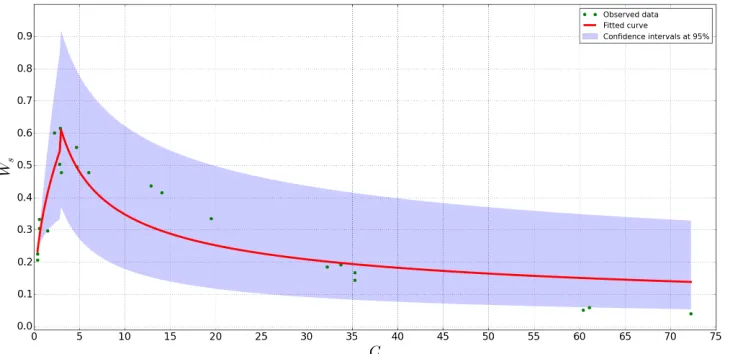
interval on the mean response at the pointx0is ˆy±1.96·se(ˆy). Figure2shows the predictions

of the mean settling velocity for cohesive sediment with confidence intervals at 95% for the nonlinear model described hereafter. A transition occurs concentrations larger than 3g·L−1_.

This regime corresponds tothe hindered regime for which we use a new piecewise continuous model:

Ws=

a1Cb1 forC <3g·L−1

a2Cb2 forC≥3g·L−1

The distributions of the parameters ai, bi are given by ai ∼ N(ˆai, σa2ˆi) et bi ∼ N(ˆbi, σ

2 ˆ_b_i), for

i= 1,2.

This methdology was also applied to the critical Shield number Θc=f(D∗) of non-cohesive sed-iment, whereD∗is the adimensional particle diameter given byD∗= d50/0.9 s−1gν−2/3,

the critical shear stress for erosionτc,e=f(C) of cohesive sediment and the Krone-Partheniades

(5)

(a)

(b)

Figure 1: 1(a)CDFs of the granulometry datadfor the fluvial part for all years 2000 to 2016. Red: upper CDFs, Blue: lower CDFs 1(b) Probability densities for the d50 and d90 for the

fluvial part of the Gironde estuary.

5 Bathymetry analysis

In spatial interpolation, the nugget effect can be attributed to measurement errors and/or spatial sources of variation at distances smaller than the shortest sampling interval. The bathymetry is then modelled applying Universal Kriging [3]. Kriging was originally introduced as a spatial interpolation method in the earth sciences, and is also known as Gaussian Process regression in machine learning. At every measurement points x, the Kriging simultaneously provides an approximation of a partially observed functionz, the kriging mean predictorµ(x), and a measure of prediction uncertainty, the kriging varianceσ2₍_x_{). The principle of Universal}

Kriging is to seez(x, y) as one realizations of a random processZ(x), and to make optimal lin-ear predictions ofZ(x) given the observations values (noisy or not) at the measurement points x. In the Universal Kriging framework,Z is generally assumed to be of the form:

Z(x) =µ(x) +G(x) =

n

X

i=1

βifi(x) +G(x) (4)

wherefi are known basis functions andGis a centered Gaussian process. In order take account

(6)

Figure 2: Predictions of the mean settling velocityWswith confidence intervals at 95% (cohesive

case), as a function of the sediment concentrationC.

assumption that the error distribution at location xis Gaussian with zero mean and variance σ2_{, the 95% confidence interval for}_Z₍_x_{) with kriging estimate}_z∗₍_x_{) is calculated as:}

P[Z(x)∈z∗(x)−1.96σ(x), z∗(x) + 1.96σ(x)] = 95% (5)

which gives upper and lower bounds for a 95% confidence interval to construct confidence envelope maps. They represent the kriging model estimation of the 95% range of potential values for any location. A set ofnmap maps of the bathymetry spatial distribution is generated

by sampling a random fieldZ∗(x) with a truncated Gaussian distribution of support [z∗(x)− 1.96σ(x), z∗(x) + 1.96σ(x)]:

Z∗(x)∼TruncatedGaussian z∗, σ(x),[z∗(x)−1.96σ(x), z∗(x) + 1.96σ(x)]

(6)

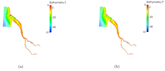
This overall procedure is repeated withndifferent levels of noise to generate bathymetry n× nmap maps of the bathymetry with the Universal Kriging. Figure 3(a) shows the original

bathymetry of the Gironde estuary and Figure3(b) shows a random field of the bathymetry generated from our method. These maps will jointly used as inputs with the other uncertain parameters in the Monte-Carlo simulations of the 2D hydrosedimentary model to estimate the uncertainties that pertained the water depthh(x, y, t).

6 Conclusion

A new methodologie processing sediment data, hydrosedimentary parameters and bathymetry data, through the use of probabilistic method, imprecise probability and non-linear regression, was presented. The main findings of our work are: (i)the highlight of the main parameters of the 2D morphodynamic models : mainly granulometry parameters (such as the sediment size d50, d90 and parameters related to the cohesive properties of the sediment),(ii)the evolution

(7)

(a) (b)

Figure 3: 3(a) Original bathymetry of the Gironde estuary. 3(b) Random field Z∗(x) of the bathymetry generated from our method.

d50andd90for different areas of the Gironde estuary,(iv)the 2D hydrosedimentary model used

for uncertainties propagation must handled mixed sediment transport(v)the characterization of the probability density distributions of the critical Shields number Θc, the settling velocity

Ws for cohesive and non-cohesive sediments, the critical shear stress for erosion τce and the

Krone-Partheniades erosion law constant M for cohesive sediment, (vi) a new model for the settlingWsfor cohesive sediment,(vii)the generation of multiple sets of the bathymetryzof the

estuary that handle the nugget effect due to measurements errors,(viii)numerical codes using OpenTurns uncertainty library [4] to process the data in Sections 2,3,4,5. Theses strategies offer flexibility to handle the variability of these experimental data are also suitable for data-driven applications since the uncertainty quantification can also be conducted from a small set of the most important parameters of the 2D morphodynamic model under consideration. They also allow to generate random sample of inputs, using their estimated probability distributions. In order to quantify the impact of the inputs uncertainties on the estimation of the water-depth h(x, y, t), the Monte Carlo method will be used to propagate these samples in a 2D morphodynamic model [6].

References

[1] Dubois, D. and Prade, H., 1988 Possibility theory.New York Plenum Press.

[2] Ferson, S. and Ginzburg, L., 1996 Different methods are needed to propagate ignorance and variability.Reliability Engineering and System Safety.54, 133–144.

[3] Montero, José and Fernández-Avilés, Gema and Mateu, Jorge, 2015 Spatial and Spatio-Temporal Geostatistical Modeling and Kriging.Princeton University Press.08

[4] Airbus-EDF-IMACS-Phimeca., 2016 Reference Guide - OpenTurns 1.7

[5] Shafer, G., 1976 A mathematical theory of evidence.Princeton University Press.

[6] Hervouet JM; Ata R., 2017 User manual of opensource software TELEMAC-2DEDF-R&D V7P2 [7] Thorn, M.F.C., 1981 Physical processes of siltation in tidal inlets.Proceedings of Hydraulic

Uncertainty Quantification in 2D Morphodynamic Model: Application to the Gironde Estuary.