ARCH-COMP18 Category Report: Stochastic Modelling

Volume 54, 2018, Pages 71–103

ARCH18. 5th International Workshop on Applied Verification of Continuous and Hybrid Systems

ARCH-COMP18 Category Report:

Stochastic Modelling

Alessandro Abate

, Henk Blom

, Nathalie Cauchi

, Sofie Haesaert

, Arnd

Hartmanns

, Kendra Lesser

, Meeko Oishi

, Vignesh Sivaramakrishnan

,

Sadegh Soudjani

_{, Cristian-Ioan Vasile}

_{, and Abraham P. Vinod}

1

University of Oxford, Department of Computer Science, Oxford, [email protected]

2 _{Delft University of Technology, Delft, The Netherlands and National Aerospace Laboratory,}

Amsterdam, The [email protected]

3 _{California Institute of Technology, Pasadena, California, USA[email protected]} 4

University of Twente, Formal Methods and Tools group, Enschede, The Netherlands [email protected]

5

Verus Research, Atlanta, Georgia, [email protected]

6

University of New Mexico, Department of Electrical and Computer Engineering, New Mexico, USA

{oishi,vigsiv}@unm.edu,[email protected]

7

School of Computing, Newcastle University, UK,[email protected]

8 _{Massachusetts Institute of Technology, Cambridge, MA, USA[email protected]} Abstract

This report presents the results of a friendly competition for formal verification and policy synthesis of stochastic models. The friendly competition took place as part of the workshop Applied Verification for Continuous and Hybrid Systems (ARCH) in 2018. In this first edition, we present five benchmarks with different levels of complexities and stochastic flavours. We make use of six different tools and frameworks (in alphabetical order): Barrier Certificates, FAUST2_{, FIRM-GDTL, Modest, SDCPN modelling & MC}

simulation and SReachTools; and attempt to solve instances of the five different benchmark problems. Through these benchmarks, we capture a snapshot on the current state-of the art tools and frameworks within the stochastic modelling domain. We also present the challenges encountered within this domain and highlight future plans which will push forward the development of more tools and methodologies for performing formal verification and optimal policy synthesis of stochastic processes.

1

Introduction

provide a set of benchmarks which we aim to push forward the development of current and future tools. To establish further trustworthiness of the results, the code describing the benchmarks together with the code used to compute the results is publicly available at

gitlab.com/goranf/ARCH-COMP.

This report summarizes results obtained in the 2018 friendly competition of the ARCH workshop1 _{for the newly established stochastic modelling group. This new category in the} friendly competition aims to push forward the verification of such models, and has the practical goal to test existing or prototype tools that verify a set of new benchmarks for such models.

Within this category, we have identified five novel benchmarks, comprising different model structures and dealing with diverse applications. All the benchmarks have varying levels of complexity, different type of stochasticity and different problem specifications. Using the current tools and algorithmic frameworks, we perform verification tasks on each of the benchmarks. The tools and frameworks used are (in alphabetical order): Barrier Certificates, FAUST2, FIRM-GDTL, Modest, SDCPN modelling & MC simulation, SReachTools. We further identify the current challenges with running the benchmarks and set out a plan for this category within upcoming rounds of the ARCH competition.

This report has the following structure. Section2presents the benchmark descriptions which include a discussion of the individual models syntax and semantics, and a presentation of the specifications of interest. Next, in Section 3 we present the participating tools or algorithmic frameworks that are used to solve instances of the individual benchmarks. We present the results for each benchmark in Section4. Finally, we identify key challenges and discuss future plans in Section5.

2

Benchmarks

We discuss a new set of benchmarks for stochastic models, and attempt a uniform syntactic presentation of them. These are: an anesthesia delivery system; a building automation system; a heated tank; a lawn mower; and a benchmark dealing with a Mars rover. Each benchmark has specific features, which we delineate first. Next, we discuss each benchmark, the different prob-lems to be solved together with specifications of interest, and different paths to their successful verification. Afterwards, the outcomes of the verification of each benchmark are presented in detail.

Specific modelling features We briefly list the key features of each benchmark:

• Anaesthesia delivery system benchmark: this benchmark is based on an automated anaes-thesia delivery problem, with a human (an anaesthesiologist) in the loop [21, 5]. The model is described in the form of a discrete-time stochastic hybrid system [1] that de-pends both the current state of the model and a history of the past input actions by the anaesthesiologist. Stochasticity comes both in the form of process noise in the underlying continuous variables and in uncertainty on the applied input action. This benchmark focuses on two verification problems: (i) the stochasticity viability problem and (ii) the stochastic first-time hitting reach-avoid problem.

• Building automation systems benchmark: this benchmark is based on a library of models describing different components within a smart building system [10]. We focus on two in-stances of possible benchmarks, both of which describe discrete-time linear systems with varying numbers of continuous state variables. The overall benchmark focuses on the verification and policy synthesis around safety properties.

• Heated tank benchmark: this benchmark is based on a known model within the area of reliability and safety [33, 34, 41]. The benchmark is composed of discrete states that transition using Poisson arrivals, depending on the failure rates of the tank and on con-tinuous variables describing the temperature and water level in the tank. The concon-tinuous variables evolve in continuous time. The difficulty in this benchmarks includes the very low probability of transitions between states due to the low failure rates.

• Lawn mower benchmark: this benchmark focuses on controller synthesis and on verifica-tion for a driverless industrial-size lawn mower [20]. While a number of diverse schemes can be used for synthesising a controller, we use one that has a simple switching mech-anism for guiding the mower between way-points in the field. We describe discrete-time dynamics of the mower together with the controller architecture. The closed-loop model fits into the framework of discrete-time hybrid systems, which has six continuous states, two discrete modes, and nonlinear vector fields in each mode. Although statistical tech-niques such as multilevel Monte Carlo method [17] can be used to verify properties of the

continuous-time dynamics presented in [20], we transform the model into discrete-time polynomial dynamics and use barrier certificates [27] for the verification task.

• Mars rover benchmark: this benchmark considers the problem of planetary exploration with a two-agent team composed of a Mars rover and a Mars helicopter, tasked to collect a set of samples from the Mars surface. Due to the high cost and risk associated with these missions, it is critical to have strong correctness and performance guarantees on the robot behaviours. This benchmark is composed of two agents described using partially observable models operating in a partially-known deterministic environment. It is tasked with complex mission specifications that could be used for real Mars rover operations [36,

35].

2.1

Anaesthesia Delivery System Benchmark

problems of interest are 1) a viability problem, in which we seek to maximise the probability of the state lying within known, safe depths of hypnosis; and 2) a reach-avoid problem, in which we seek to maximise the probability of the state reaching a desirable depth of hypnosis, while staying within safe hypnosis depths.

2.1.1 Model formulation

We denote a discrete-time time interval by _N[a,b] for a, b ∈ N and a ≤ b, which inclusively

enumerates all integers in between (and including) a and b. We denote non-random vectors with an overline, random variables with bold case, random vectors with bold case and an overline, In ∈Rn as the identity matrix, the Cartesian product of the setG with itselfk ∈N

times asGk_{, and the cardinality ofG with|G|.}

Propofol concentration in the patient with external drug administration The con-centration of a drug administered to a patient is often represented by a multi-compartment model [26]. The concentration of Propofol in different compartments of the body are modelled using the three-compartment pharmacokinetic system [32,30,21]:

˙

x(t) = 

 

−(k10+k12+k13) k12 k13

k21 −k21 0

k31 0 −k31 

 x(t) +

   1 V1 0 0  

u(t) (1)

The state x(t) = [x1(t) x2(t) x3(t)]> ∈ X = R3 represents the concentration in each of the

three compartments. The inputu(t)∈ U ⊂_Rrepresents the rate of administration of Propofol, andV1, kij∈R(i, j∈ {1,2,3}) are patient dependent parameters. Table1lists the parameter

values determined for a 11-year old child weighing 35 kilograms from the Paedfusor dataset [2].

k10 k12 k13 k21 k31 V1 0.4436 0.1140 0.0419 0.0550 0.0033 16.044

Table 1: Model Parameters from the Paedfusor dataset.

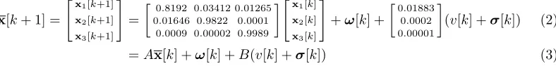
Automated anaesthesia delivery and anaesthesiologist in the loop We discretise the continuous-time model (1) using a zero-order hold with a time-step ofTs= 20s, and presume that the anaesthesiologist input occurs exactly at the sampling instant. The discrete-time approximation of (1) (using parameter values given in Table1) is

x[k+ 1] =

"_x1[k+1]

x2[k+1] x3[k+1] #

=

0.8192 0.03412 0.01265 0.01646 0.9822 0.0001

0.0009 0.00002 0.9989 "x1[k]

x2[k] x3[k] #

+ω[k] +

0.01883 0.0002 0.00001

(v[k] +σ[k]) (2)

=Ax[k] +ω[k] +B(v[k] +σ[k]) (3) The automated input is v[k] ∈ V, and the input from the anaesthesiologist is the random variableσ[k]∈ H, a finite set that contains all possible dosages the anaesthesiologist can give at the current time instant k. We presume the anaesthesiologist may either choose to not provide a bolus dosage or give a bolus dosage at the rate of 30 mg/min forTsseconds resulting in a dose of 10 mg being administered during the interval of Ts seconds. The zero-mean Gaussian random vectorω[k] ∼ N(0, M) with known covariance matrix M ∈ R3×3 accounts

system matrix A ∈ _R3×3 _{and input matrix B ∈}

R3×1. The bolus dosage ensures that the

required concentration of the drug can be achieved and maintained throughout the duration of administration with the help of a trained anaesthesiologist [26]. In this benchmark problem, we choose V = [0,7] mg/min, H={0,30} mg/min, and M = 10−3_I

3. The continuous state x[k] = [x1[k]x2[k]x3[k]]> ∈ R3 is a random vector due to the stochastic human input σ[k]

and the noiseω[k].

Probabilistic model of the anaesthesiologist actions We model the bolus dosage,σ[k], as a stochastic process that depends on the current statex1[k] and the past values ofσ[·]. We also assume the anaesthesiologist uses a concentration threshold parameter α to decide if a bolus dosage is to be given. Table2describes a fictitious anaesthesiologist model, through the probability of applying the bolus dosage under various conditions.

Probability of applying

Conditions the bolus dosage

0.95 x1[k]> α and 0/1 bolus dosage was given in past three minutes 0.90 x1[k]≤α and 0 bolus dosage was given in past three minutes 0.50 x1[k]≤α and 1 bolus dosage was given in past three minutes

0 otherwise

Table 2: A model of the anaesthesiologist’s decision to apply a bolus

2.1.2 Discrete-time stochastic hybrid system model

We write (2) as a discrete-time stochastic hybrid system (DTSHS) [1] by defining the tuple H(X,Q,V, Tx, Tq), where

1. X =R3is the continuous state space,

2. Q={0,1}9_{is the discrete state space,}

3. S=Q ×X is the hybrid state space,

4. V = [0,7] mg/min is the admissible controls for the automation,

5. Tq :Q × S →[0,1] is a discrete stochastic transition kernel onQgiven the current hybrid state (q, z)∈ S and is defined by (5), and

6. Tx:B(X)× S × V →[0,1] is a Borel-measurable stochastic kernel on X given given the current hybrid state and the current automation action (q, z, v)∈ S × V and is defined by (6).

state are described by

q[k+ 1] =         

0 0 . . . 0 0 1 0 . . . 0 0 0 1 0 . . . 0

..

. . .. . .. . .. 0

0 . . . 0 1 0         

q[k] +       1 30 0 .. . 0      

σ[k]. (4)

The binary counter stateq[k] is a random vector sinceσ[k] is a random variable. We incorporate the anaesthesiologist model in Table2 to define the discrete transition kernel,

Tq(q0, q, z) =                             

0.95 q0 = [1q_1:8]>,kqk₁≤1, z1> α 0.05 q0 = [0q1:8]

>

,kqk₁≤1, z1> α 0.9 q0 = [1q_1:8]>,kqk₁= 0, z1≤α 0.1 q0 = [0q1:8]

>

,kqk₁= 0, z1≤α 0.5 q0 = [1q_1:8]>,kqk₁= 1, z1≤α 0.5 q0 = [0q1:8]

>

,kqk₁= 1, z1≤α 1 q0 = [0q_1:8]>,kqk₁= 2

0 otherwise

(5)

where q_1:8 is the vector [q₁ . . . q₈]> ∈ {0,1}8, and z1 ∈Ris the first component of z. From

(4), the first component ofq0₁is 1 if the current action of the anaesthesiologistσ[k] is 30 (apply bolus); otherwise,q0₁ is 0.

The stochastic continuous state transition kernel, Tx, can be defined using (2) and the probability measure over (_R3_,B(

R3)). Sinceω[k]∼ N(0, M), if the current automation input

isν∈ V, the current continuous state isz∈ X, and the discrete stateq∈ Q

Tx(·|q, z, ν)∼ N(Az+B(ν+ 30q1), M). (6)

2.1.3 Verification problem

Consider a safe setK ={z∈ X : 1≤z1≤6,0≤z2≤10,0≤z3≤10} ⊂ X, and a target set T ={z∈ X : 4≤z1≤6,8≤z2≤10,8≤z3≤10} ⊂ X.

Problem 2.1.1. (Stochastic viability problem)Given an initial state(q[0], z[0])∈ S, com-pute the maximum probability of guaranteeingx[k]∈ Kfork∈_N[0,10], and design an admissible

controller that achieves this probability.

2.2

Building Automation System Benchmark

The Building Automation System (BAS) benchmark is a modular and extendable benchmark constructed from a library of stochastic models representing the different components making up a BAS. The library of models is presented in [10] and the reader is referred to the afore-cited paper for more details. Using this library of models we setup two instances which aim to address verification and policy synthesis respectively. We denote the first instance as CS1BAS, while the second instance as CS2BAS. For each instance (i) we establish the dynamics of the models, (ii) the specification of interest, and (iii) we describe possible solutions.

2.2.1 CS1BAS: Model

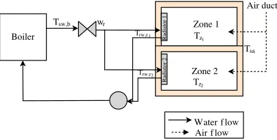
Figure 1: BAS setup for the first case study

We consider two zones, each heated by one radiator and with a common supply air, as portrayed in Figure1. The model is described as stochastic linear discrete-time model

x[k+ 1] =Ax[k] +Bu[k] +Q+ ΣW[k] (7)

ys[k] =

1 0 0 0

0 1 0 0

x[k], (8)

with a uniform sampling time ∆ = 15 minutes. Here, the matrices A, B, Q are properly sized andΣ =diag([(√∆σz1)

2₍√_∆σ

z2)

2₍√_∆σ

rw,r1)

2₍√_∆σ

rw,r2)

2_{])encompasses the variances of the}

process noise for each state. W = w1 w2 w3 w4 T

are independent Gaussian random variables, which are also independent of the initial condition of the process. The exact matrix values are kept within the ARCH repository.

2.2.2 CS1BAS: Specification

We consider the stochastic safety property: to decide whether traces generated by the models remain within a specified safe set for a given time period. Specifically, this is described using the PCTL property:

Φ :=P=p[≤N=1.5hoursS] (9)

where pis the probability of satisfaction, S is the safe set is described as an interval around the temperature set-pointTSP = 20oC ±0.5oC, specifically,

S= 

  

19.5 20.5 19.5 20.5 19.5 20.5 19.5 20.5 

  

We have defined the acceptable probability of the specification to be true forp≥0.9.

2.2.3 CS2BAS: Model

In this second case study we focus on the stochastic dynamics of the zone component. The model is a discrete-time model with a sampling time ∆ = 15 minutes, and takes the form of

xc[k+ 1] =Acxc[k] +Bcuc[k] +Fcdc[k] +Qc (10)

yc[k] =

1 0 0 0 0 0 0

xc[k]. (11) Here the continuous state variable xc is composed of 7 states representing the zone and wall temperatures, the inputuc corresponds of the fan supply rate having a dimension of 1. The disturbance vectordc has a dimension of 6 which represent external heat sources (weather, oc-cupancy, radiators), whileQc represents constant additive terms within the model. We model the disturbances as random external effects following Gaussian distributions with a meanµand varianceσ, affecting the room temperature dynamics asTout[k]∼ N(µ= 9, σ= 1), Thall[k]∼ N(µ = 15, σ = 1), CO2i[k] ∼ N(µ = 500, σ = 100), i ∈ {1,2}, Trw,ri[k] ∼ N(µ = 35, σ = 5), i∈ {1,2}.

2.2.4 CS2BAS: Specification

We would like to synthesise a policy ensuring that the temperature within zone 1 does not deviate from the set point by more then 0.5o_{C over a time horizon equal to 1.5 hours (i.e}

N = 6). This can be translated into following PCTL specification: Φ :=P=p[≤N=6|Tz1−TSP| ≤0.5]

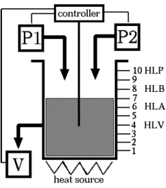
Figure 2: Illustration of the heated tank benchmark (version 5)

2.3

Heated Tank Benchmark

The Heated Tank benchmark is a well-known example problem from the dynamic reliability literature [33,34,41]. The system consists of a tank containing liquid whose level is influenced by two pumps and one valve managed by a controller (see Fig.2). The purpose of the liquid in the tank is to absorb and transport the heat from a heat source; this means that under nominal conditions one of the pumps produces a constant inflow of cool liquid, and a similar flow of heated liquid leaves the tank through the valve.

2.3.1 Continuous-time hybrid-state process model

The general model adopted for this heated tank system is that of piecewise deterministic Markov processes (PDMP). The discrete-valued process θt consists of components for the two inflow pumpsP1andP2, the outflow valveV, the controllerC and the tankT, i.e.

θt=hθP1,t, θP2,t, θV,t, θC,t, θT ,ti.

The Euclidean-valued processxt has twoR-valued components, one for liquid heightxH,t and another for liquid temperaturexT ,t. These Euclidean-valued components evolve according to the following switching differential equations:

˙

xH,t= (χP1,t+χP2,t−χV,t)·q with initial conditionxH,0=Hinit and

˙

xT ,t= ((χP1,t+χP2,t)·(Tin−xT ,t)·q+Ein)/xH,t with initial conditionxT ,0= 15 2_/3◦_C

where χU,t indicates if unit U ∈ {P1, P2, V} is working or not (i.e. χU,t = 1 if unit U is working and 0 otherwise),qis the flow parameter, Tin = 15◦C is the inflow temperature, and

Ein= 1

◦_Cm

h is the heat source parameter. The differential equation forxT ,t is from [41]. The (rare) event probabilities to be estimated on a finite time interval [0, tend] are:

• the dryout probabilityP(∃t∈[0, tend] :xH,t≤Hdryout),

• the overflow probabilityP(∃t∈[0, tend] :xH,t≥Hoverflow), and

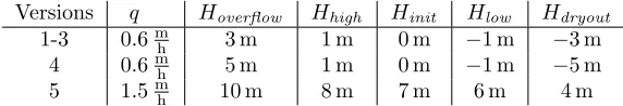
Versions q Hoverflow Hhigh Hinit Hlow Hdryout

1-3 0.6m

h 3 m 1 m 0 m −1 m −3 m

4 0.6m_h 5 m 1 m 0 m −1 m −5 m

5 1.5m_h 10 m 8 m 7 m 6 m 4 m

Table 3: Parameter values for different versions of the heated tank benchmark

The evolution of the two R-valued state componentsxH,t and xT ,t depends on the evolution of the indicator processes χP1,t, χP2,t and χV,t. Codetta-Raiteri [11] identified five different versions for the evolution of these indicator processes and the parameters. The values used across the five versions for the flow and level parameters are listed in Tab. 3. We describe all other differences between the five versions in the following subsections.

2.3.2 Version 1: Baseline

Each of the three unitsP1,P2 andV has the following set of four discrete modes: ΘU ={On,Off,StuckOn,StuckOff}.

The initial condition is

θP1,0=On∧θP2,0=Off ∧θV,0=On.

The switching fromOn toOff and vice-verse is managed by the controller.

In addition to this switching, there are four exponentially distributed failure switching pos-sibilities: from On to StuckOn, from On to StuckOff, from Off to StuckOff, and from Off

to StuckOn. Each of these failure transitions happens at rate ˆλP1 = 1/438 h for P1, at rate ˆ

λP2 = 1/350 h forP2, and at rate ˆλV = 1/640 h forV.

The controller mode processθC,t switches between the following three configurations: ΘC ={Normal,Increase,Decrease}.

The initial condition of the controller isθC,0=Normal.IfxH,t≤HLow thenθC,tswitches from

Normal or Decrease toIncrease. IfxH,t ≥HHigh thenθC,t switches from Normal or Increase toDecrease. The low and high liquid level parameter values areHLow= 6 m andHHigh = 8 m.

The control law of the controller is a function ofθC,t. IfθC,t=Normal then the controller does not try to influence the pumps and valve. IfθC,t =Increase then the controller aims to increase the height of the liquid in the tank, by switching both pumps on, and by switching the valve off. IfθC,t=Decreasethen the controller aims to decrease the height of the liquid in the tank, by switching both pumps off, and by switching the valve on. The switching by the controller has no effect on unitU if it is in failure modeStuckOn or StuckOff.

2.3.3 Version 2: Mode-dependent Failure Rates

Compared to version 1, the failure rates now depend on the current mode of the respective component, and the two different kinds of failures occur with different rates. The following modifications are made to the rates: ForP1, the rate to move fromOff toStuckOn is 20·λˆP1 and the rate to move fromOff to StuckOff is 200·ˆλP1. For P2, the rate to move from On to

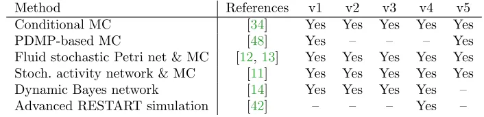
Method References v1 v2 v3 v4 v5

Conditional MC [34] Yes Yes Yes Yes Yes

PDMP-based MC [48] Yes – – – Yes

Fluid stochastic Petri net & MC [12,13] Yes Yes Yes Yes Yes Stoch. activity network & MC [11] Yes Yes Yes Yes Yes

Dynamic Bayes network [14] Yes Yes Yes Yes –

Advanced RESTART simulation [42] – – – Yes –

Table 4: Methods previously applied to the heated tank benchmark

2.3.4 Version 3: Controller Failure on Switching

Relative to version 1, each time the controller’s law is to trigger a switching of one or more of the units P1, P2 and V, it is assumed that this controller action will be realized with a probability of 90 % only. This means that there is a 10 % probability that a required switch is not implemented forP1,P2andV.

2.3.5 Version 4: Controller-Triggered Repairs

Relative to version 1, it is assumed that the control laws underIncrease andDecrease include triggering a repair of any unit (P1,P2 or V) if it cannot be switched. The duration of such a repair is assumed to be exponentially distributed, with a mean of 5 hours. Upon repair of unit

U, the controller implements the desired switching for this unit.

2.3.6 Version 5: Temperature-Dependent Failure Rates

Relative to version 1, the static failure rates ˆλP1, ˆλP2 and ˆλV are replaced by temperature-dependent failure rates ˆλP1·α(xT ,t), ˆλP2·α(xT ,t) and ˆλV ·α(xT ,t), respectively, where

αxT ,t=

b1·ebc·(xT ,t−20)+b2·e−bd·(xT ,t−20)

/(b1+b2) (12)

with parameter valuesb1= 3.0295,b2= 0.7578,bc = 0.05756 andbd = 0.2301. Note that, in order to resolve a typo in [11], for the above equation we followed [41].

2.3.7 Results from the Literature

2.4

Lawn Mower Benchmark

Here we describe dynamics of a lawn mower adapted from [20]. A conceptual model of the driverless lawn mower is shown in Fig. 3(a). The lawn mower is steered by controlling the velocity separately on the two driving wheels. A sketch of the vehicle is shown in Fig. 3(b)and its chassis and caster wheels are shown in Fig. 3(c).

(a) (b) (c)

Figure 3: Lawn mower schematics [20]

2.4.1 Dynamical model

The dynamic response of the lawn mower can be described by a 6-dimensional nonlinear stochas-tic difference equation

x[k+ 1] =f(x(k), v(k), w(k)), k= 0,1,2, . . . (13)

wherex(·)∈R6is the state,v(·) = [Vr(·), Vl(·)]T ∈R2≥0is the input, andw(·)∈R

2_{is the noise.}

The vector fieldf :_R6_×

R2≥0×R2→R6 is defined by the following elements

f1(x, v, w) =x1+

Ts

Izz

Af ysin

x6+

π

2

a+ 2Cγtan

2(x₂−bx₁) (Vr+Vl)

b

,

f2(x, v, w) =x2+

Ts

M

Af ysin

x6+

π

2

−2Cγtan

2(x₂−bx₁) (Vr+Vl)

−Ts(Vr+Vl) 2 x1,

f3(x, v, w) =x3+

Ts(Vr+Vl)

2 cos(x5), (14)

f4(x, v, w) =x4+

Ts(Vr+Vl)

2 sin(x5),

f5(x, v, w) =x5+Ts _V

r−Vl 2D +x1

+w1,

f6(x, v, w) =x6−

Ts(Vr+Vl)

2d cos(x6)−

Ts(Vr−Vl)(d+ p

D2_{+ (a+b)}2_sin(x 6))

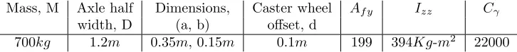
Mass, M Axle half Dimensions, Caster wheel Af y Izz Cγ

width, D (a, b) offset, d

700kg 1.2m 0.35m, 0.15m 0.1m 199 394Kg-m2 ₂₂₀₀₀ Table 5: Lawn mower parameters

where x1, x2, x3, x4, x5, and x6 are respectively yaw, yaw rate, x, y, angle of vehicle with respect tox-axis (θ), and relative orientation of caster wheel (β), respectively. Thew1 andw2 are noises in orientation and angle of caster wheel generated due to uneven ground surface. Vr andVlare the control inputs representing velocity of right and left driving wheels, respectively. ParameterTs is the sampling time. The remaining parameters are listed in Table5.

2.4.2 Controller mechanism

The main objective for the lawn mower is to cover a given area as soon as possible. This can be seen as a path planning problem and is usually achieved by specifying a set of way-points, and the task of the controller would be to move from an initial position in the vicinity of the current way-point to the vicinity of the next way-point. We provide simple On-Off type controller for the lawn mover to reach the desired position (xd, yd). Consider base velocity Vb and boost velocityVd. The control inputs that is velocities of right and left wheel are given as

Vr=Vb+Vdsgn(sin(θd−x5))

Vl=Vb−Vdsgn(sin(θd−x5)), (15) whereθd= atan2((yd−x4),(xd−x3)) and atan2 is the four-quadrant inverse tangent.

2.4.3 Specification of interest

The controller of the previous subsection does not take into account avoiding obstacles and preventing collision with boundaries of the area. Here we define a specification that computes the probability of avoiding obstacles over finite-time traces of the system.

The state space of the system isX=R6. Consider the desired location (xd, yd) = (−10,−5) with selection ofVb= 2 andVd= 1.5 We also consider the regionX0= [−0.5,0.5]2×[−1,1]2× [−π, π]2 for the initial state of the system and X1 = [−0.5,0.5]2×[−4,4]×[2.5,4]×[−π, π]2 for the obstacles or one of the boundaries of the area. The set of atomic propositions is given by Π = {p0, p1, p2} with labeling function L(xi) = pi for all xi ∈ Xi, i ∈ {0,1,2}, with

X2:=X\(X0∪X1) . The objective is to compute a lower boundα >0 on the probability that the solution process of lengthN = 200 satisfies the safe LTLf formulap0∧≤200¬p1:

Figure 4: Labelled map of a campaign where blue and purple mark regions containing science targets for the rover and orange area shows the region in sand.

2.5

Mars Rover Benchmark

We introduce the problem of planetary exploration with a two-agent team composed of a Mars rover and a Mars helicopter, tasked to collect a set of samples from the Mars surface. Due to the high cost and risk associated with these missions, it is critical to have strong correctness and performance guarantees on the robots’ behaviours. To aid in this objective, we give a mission specification framework and formally encode complex mission specifications used for real Mars rover operation. The logic of choice is syntactically co-safe Linear Temporal Logic (scLTL) defined over predicates in belief space [28,43]. This approach allows us to capture temporal and uncertainty constraints ranging from science campaign (e.g., getting science results from specific regions) to operational constraints such as maintaining certain accuracy over the vehicles’ state and the environment, inter-agent distance, and energy level.

For a first and more accessible case study, we consider a simplified version of the full spec-ification set. Additionally, the rover is assumed to have stochastic motion and perception, and is tasked with collecting samples from a partially-known deterministic environment. The helicopter provides support by exploring the environment on-demand. Exploration is neces-sary if insufficient knowledge is available to synthesise a control policy with sufficient success probability.

2.5.1 Scientific Mars Mission

The set of requirements below specify a potential science campaign. We say that actions taken by the rover or copter have an associated risk (r) of a certain (hidden) event, the requirements impose bounds on the risks associated to specific events that the Mars rover copter mission can take.

1. Rover must get a type A sample from a type A target and it must get one type B sample of a science target of type B. Areas that potentially include either type A or B are shown in purple and blue, respectively, in Fig.4. They represent areas for potentially high-science-value rock/soil samples that need to be collected.

2. Rover must maintain the variance of its state belowΣmax. This specification is to maintain accuracy along the mission, and reduce the risk of unexpected events.

Rock (CFA)

Slope (degrees)

7%

14%

10

20

Figure 5: Speed Constraints for Slope vs Rock CFA (Cumulative Fractional Area). High speed (green), Low speed (yellow) and Stop (red).

4. Rover must follow speed constraints. Rover’s maximum speed is a function of the cumu-lative fractional area of rocks, and the terrain slope, see Fig. 5.

5. Mars helicopter must avoid landing near hazards. These hazards include, inter alia, large rocks, deep sands, and steep slopes. More precisely, the helicopter cannot land somewhere, where it has a risk probability greater than r5 of landing within x5 meters of a hazard zone.

6. Helicopter must maintain a minimum distancedmin and a maximum distancedmaxfrom

the rover. The purpose of this specification is to protect the primary asset of the mission: the rover, which carries all vital science instruments. The helicopter should not pose any risk for the rover in case of helicopter failure, but should also maintain communication range.

2.5.2 Introduction: A formal Belief space planning problem

In this section, we define the planning problem under uncertainty and in partially-observable environments. We start by reviewing Partially-Observable Markov Decision Process (POMDP) and associated synthesis problem. Then, we present the belief-based linear temporal logic (LTL) properties to be used for mission planning.

POMDP. Let us denote the system state, action, and observation at the k-th time-step by

x[k], u[k], z[k], respectively. Let

x[k+ 1] =g(x[k], u[k], w[k]) (16)

z[k] =h(x[k], v[k]) (17) denote the system dynamics and measurement models, where w[k] ∼ pw(·|x[k]) and v[k] ∼

pv(·|x[k]) denote the state-dependent process and observation noise. Due to the observation noise, the best one can infer about the system state is a probability distribution over all possible states, referred to asbelief b[k] =p(x[k]|i[k]) with historyi[k] :={(u, z)0:k}. The belief space (i.e., the set of all beliefs) is denoted by B. Belief is typically evolved using a recursive filter

denoted byτ as

As is common, one can generally assume that the belief space is a Polish space2 _{and that the} recursive filter is a Borel measurable mapping.

Belief-space LTL. Letb =b[0]b[1]b[2]. . . ∈ Bω be a belief sequence, and AP be finite set

of atomic propositions. Each elementf ∈ AP is a predicate over the belief space B, and we

say that a beliefb satisfies f if f(b) =>, where> is the truth Boolean value. Moreover, the predicate functionsf must be Borel measurable mappings. Using the set of belief-based atomic propositionAP, we defined mission specifications using scLTL, which has as syntax

φ:=> | f | ¬f | φ1∧φ2|φ1Uφ2 | φ

For convenience, we use the additional operators: φ1∨φ2 ≡ ¬(¬φ1∧ ¬φ2), ♦φ≡ > Uφ, and 2φ≡ ¬♦¬φ, where ≡denotes semantic equivalence.

Control synthesis problem. The control synthesis problem for the POMDP with belief-based LTL specifications can be formulated as follows:

Problem 2.5.1. Let φ be a given LTL formula and let the robot evolve according to dynam-ics (16), with observation dynamics (17), and using a Bayesian filter defined by (18). Find a policyµ∗ such that

µ∗= arg max µ∈M

P r[b|=φ] subject to (16),(17),(18). ₍₁₉₎

2.5.3 POMDPs modeling rover, helicopter, and environment

In this section, we define the models for the Mars rover robot and helicopter robot, and the Martian environment, where the two robots must perform science campaigns such as the one described in Sec.2.5.1.

The state of this combined system model is denoted as x= (xr, xc, m) and is comprised of the rover statexr, the helicopter state xc, and the unknown environment statem. Each of these states is not exactly known. Due to the noise in the robots’ motion and perception, the best one can infer about the overall system state is its belief, i.e., the probability distribution over all possible states, denoted byb[k] =p(x[k]|i[k]), where the history is given composed of the past actionsuand the past observationsz, that is,i[k] :={(u, z)0:k}.

Based on joint belief over rover, helicopter, and the environment,b we can compute three separate marginalised beliefs for each of the models as

br=p(xr|i[k]) = rover position distribution

bc=p(xr|i[k]) = copter position distribution

bm=p(m|i[k]) = environment belief

(20)

Rover model. The kinematics of the rover can be described using the special Euclidean group of planar motions, i.e. SE(2). The rover’s state xr _{= (p}r_{, v}r_{) is a combination of its pose} parameterised aspr_∈

R2×[−π, π) and its velocityvr∈R3. The dynamics of the rover can be

represented by a unicycle model





x[k+ 1]

y[k+ 1]

ϕ[k+ 1] 

= 



x[k] +vcos(ϕ[k]δk y[k] +vsin(ϕ[k]δk

ϕ[k] +ωδk



+w, (21)

wherev(velocity) andω(angular velocity) are the inputs andw∼ N(0, Q) is Gaussian process noise.

Helicopter model. Similarly to the rover, the helicopter’s kinematic are given viaSE(3) and its statexc_{= (p}c_{, v}c_{) includes the pose parameterised asp}c_∈

R3×[−π, π)2×[0, π], and velocity

vc_∈

R6.

Simplified rover and copter belief models For simplicity and practical implementation, we will assume that the belief about the state of the rover’s and helicopter’s pose and velocity are maintained using extended Kalman filters [29]. Thus, the beliefs are normal distributions parameterised by mean and covariance, i.e.,br≡(ˆxr,Σr) andbc≡(ˆxc,Σc), respectively. Environment and sensor model. The Martian environment contains N regions of type

A, B, ... More specifically, every region is labeled by a single type indicating whether it could potentially include either samples of that type, or hazards in case of hazard typed regions. Thus the state of the environment comprises of 0,1 values for each of the regions, 0 indicates the absence of the type whereas 1 signifies its presence. Therefore the set of states of the environment is given asR:={0,1}N _{with elements m∈ R. Over the time of a Mars mission} the unknown environment state remains constant.

Let thei−th region be represented by a bounded connected setRi_⊂

R2, and assume that

Ri _andRj _{are disjoint sets iffi6=j.}

Furthermore, we use the notation RA to indicate the collection of sets of type A and RB the collection of sets of typeB.

At every time instant the rover, or helicopter, can decide to make an observation of one of the regions. For thei-th region, we can obtain measurementszi∈ {0,1}of the semantic labels over the environment by running classifiers on the images collected from the camera on the rover. The false rate of these measurement is as follows:

p(zi6=xi_true) = 1 2dmax

min{di, dmax} (22)

where di _{is the relative distance to the i−th region and wherex}i

true ∈ {0,1} is the true, but unknown, state of that regions. Where dmax is the largest distance from which you still get informative images.

2.5.4 Mission Specification in LTL

In this section, we define the LTL predicates and properties corresponding to the mission specifications described in Sec.2.5.1.

The overall specificationφfor the campaign executed over the span ofT time units:

φ:=2≤T(funcert∧φsaf ety∧φoperational)∧φscience (23) which expresses the mission where the science objective φscience needs to be satisfied and we need to maintain a desired level of accuracy, safety, and operational constraints until the end of the mission as expressed byfuncert, φsaf ety, andφoperational, respectively. The operator2≤T denotes the bounded time invariance.

Science: The science objective in this campaign is to collect one sample from each of the high-valued science areas A and B. The rover can obtain a sample from a region once it has entered the region and if the sample type is present in the region. Thus we can specify its behavior next. Consider the following predicate to indicate the position of the rover with respect region

iand riskgiven as

fi,(br) :=

1 if_P(pr_∈R

Furthermore, we denote a predicate associated to the observation of thei-th region as (zi_{= 1).} Thus we finally have the mission specification as

φscience :=♦≤T _

i∈A

(zi = 1)∧fi,1−(br)

∧ ♦≤T _ i∈B

(zi= 1)∧fi,1−(br)

. (24)

Uncertainty: The uncertainty objective is to maintain the desired level of accuracy on the state estimates.

funcert:=tr(Σr)<Σrmax withbr≡(ˆxr,Σr),

funcert:=tr(Σc)<Σcmax withbc≡(ˆxc,Σc). (25) Safety: Space applications fall into the category of safety-critical applications. Thus, main-taining the safety of systems during operation is a paramount objective of the mission. We express the safety specification as:

φsaf ety :=φkeepout∧fnear. (26) The keepout part of the specification is given as follows. The distance from risky regions in the map such as non-traversable obstacles, sandy areas with a risk of getting stuck, cliffs, and high-slope areas, is captured by propertyφkeepout. We define keep-out constraints for the rover:

φkeepout:= ^

i∈O

(bmi ≥0.05)→ ¬f(i,0.05)(br) (27)

3

Participating Tools & Frameworks

The tools and frameworks used in the category Stochastic Modelling are introduced subse-quently in alphabetical order.

Barrier Certificates The paper [27] provides a systematic approach of using barrier certifi-cates for algorithmic verification of stochastic systems against a wide class of temporal proper-ties. It provides a method for computing lower bounds on the probability that a discrete-time stochastic system satisfies a given safe LTL specification over a finite time horizon. This is achieved by first decomposing the specification into a sequence of simpler verification tasks based on the structure of the automaton associated with the negation of the specification. Then it uses barrier certificates for computing probability bounds for simpler verification tasks, which are further combined to get a lower bound on the probability of satisfying the original specification. Computation of barrier certificates can be performed for polynomial dynamics using sum-of-squares optimizations.

FAUST2 The toolFormal Abstractions of Uncountable-STate STochastic processes (FAUST2) [39] generates formal abstractions of discrete-time Markov processes (dtMP) defined over con-tinuous state spaces. The dtMP model is abstracted into a finite-state Markov chain or a Markov decision process. The abstract model is formally put in relationship with the con-crete dtMP via a user-defined maximum threshold on the approximation error introduced by the abstraction procedure. FAUST2 _{allows exporting the abstract model to well-known} probabilistic model checkers, such as PRISM [31] or STORM [16]. Alternatively, it can han-dle internally the computation of PCTL properties (e.g. safety or reach-avoid) over the ab-stract model, and refine the outcomes over the concrete dtMP via a quantified error that depends on the abstraction procedure and the given formula. The toolbox is available at

https://sourceforge.net/projects/faust2/

FIRM-GDTL The feedback information roadmap tool for Gaussian distribution temporal logics supports the path planning of partially observable robots. The python-based toolbox can handle several kinds of robots The tool is available at https://github.com/wasserfeder/ gdtl-firm/tree/dev-mars-fsa

Modest Toolset The Modest Toolset [25] supports the modelling and analysis of hybrid, real-time, distributed and stochastic systems. A modular framework centred around the stochastic hybrid automata formalism [24] and supporting the JANI specification [8], it provides a va-riety of input languages and analysis backends. The modelling formalism at the core of the Modest Toolset is the model of networks of stochastic hybrid automata (SHA), which combine nondeterministic choices, continuous system dynamics, stochastic decisions and timing, and real-time behaviour, including nondeterministic delays. A wide range of well-known and ex-tensively studied formalisms in modelling and verification can be seen as special cases of SHA e.g. STA (stochastic timed automata), PTA (probabilistic timed automata) and PA/MDP (probabilistic automata/Markov decision processes). The toolset can can be obtained from

SDCPN modelling & MC simulation Stochastically and Dynamically Coloured Petri Nets (SDCPN) [18, 19] have been developed in support of the compositional modelling of any Gen-eralized Stochastic Hybrid Automaton [9]. In combination with conditional and rare event MC simulation, SDCPN modelling has successfully been applied for the quantitative risk modelling and assessment of future air traffic management designs, e.g. [4].

SReachTools A MATLAB toolbox to tackle various problems in stochastic reachability. It aims to support the following problems: Stochastic reach-avoid problem [40, 1] (guarantee-ing safety for stochastic systems), Lagrangian methods-based underapproximation [22], Fourier transforms-based underapproximation [46, 47], and forward stochastic reachability [45] (char-acterizing the stochasticity of the state at a future time of interest). The tool is available at

https://unm-hscl.github.io/SReachTools/.

4

Results

We present the results obtained for each benchmark using the tools highlighted in Sec.3. Given the different modelling structures, the dissimilar stochastic elements and that most of the tools and frameworks are tailored to a specific task, not all tools or frameworks could be applied to each benchmark. Consequently, in this section we present the results of the specific tools and frameworks when a solution can be computed.

4.1

Anaesthesia benchmark

4.1.1 Verification and controller synthesis using SReachTools

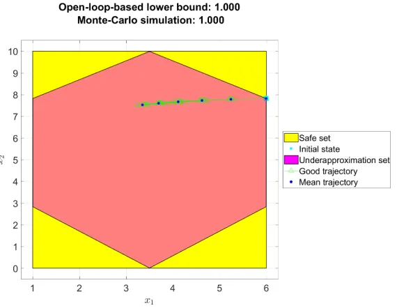
We solve Problem2.1.1by synthesising an open-loop controller as well as a polytopic underap-proximation of the true stochastic reach-avoid set. Figure6 shows the obtained 2-dimensional underapproximative polytope (x3[0] = 5) of the stochastic reach-avoid set for a probability threshold of 0.99 using 10 direction vectors. This computation took ∼ 77 seconds on an In-tel Xeon CPU with 3.4GHz clock rate and 32 GB RAM. Figure 7 shows the Monte-Carlo simulation-based validation of the open-loop controller from one of the vertices.

The SReachTools code to solve Problem2.1.1is available on [44].

4.1.2 Verification using FAUST2

We perform probabilistic reachability analysis for the specification,

Φ :=P=p[≤N S]

with

S= 



1 6

0 10 0 10 

.

Figure 6: Polytope containing a subset of the initial states from which an open-loop controller exists that solves Problem2.1.1.

(a) N = 1

(b) N = 5

Figure 8: Partition of the safe set along with the optimal safety probability afterN time steps

Next, we generate the optimal policy for the given abstractions. The input has been discre-tised into two points: [3.5 7]. We result with an optimal policy in the form of a look up table which describes the optimal action to take for each grid point and time horizon. We show the corresponding plot for a time horizonN = 1 in Fig.4.1.2.

Figure 9: Input action lookup table atN = 1

4.2

Building Automation System benchmark

4.2.1 CS1BAS: Results

The results obtained using the individual tools are presented hereunder.

Verification using FAUST2 Here, we compute the optimal safety probability for the safe set described in within the PCTL property described using (9) by applying FAUST2. Here, FAUST2 abstracts the safe set into uniform partitions over which the safety probabilities are given. The obtained results are depicted in Fig.10. The abstraction and computation of the value functions took 21.08 seconds to be generated. The abstraction consists of 1444 representative points for the continuous variables, while it consists of 25 representative points of the input.

19.5 20 20.5

19.5 20 20.5

Tz1( o_C) Tz

2

(

oC

)

0.6 0.8

Prob.

4.2.2 CS2BAS: Results

For the model described using (11) and the given specification, we aim to synthesise a policy that maximises the safety probabilityp. This synthesis goal can be computationally hard due to the number of continuous variables making up (11).

Verification using FAUST2 _{In order to make use of the FAUST}2_{, we perform policy synthesis} via abstractions and (ε, δ) simulation relations [23]. The (ε, δ) pair providing the optimal trade off is obtained using an abstract model with 1 continuous variable and corresponds to (0.28592,

10−2_{). Next, we use FAUST}2_{to perform a grid-based computation of the safety probability on} the abstract model and obtain a model of size 5943640 with an overall accuracy of 0.15. Over this approximation we synthesise the optimal policy for the abstract model which results in a safety probability ofp0= 1. We refine the obtained policy [23] such that it can be applied to the original model (11). The overall process results in Φ being satisfied with a safety probability ofp=p0η−N δ = 0.7900, whereη is the abstraction error introduced by FAUST2. The total computational time taken to obtain the optimal policy was 185.65 seconds.

4.3

Heated Tank benchmark

Versions 1 through 4 of the Heated Tank benchmark have been evaluated using both the Modest and the SDCPN based MC simulation approach. On this basis we identify similarities and differences regarding:

• understanding of the Heated tank benchmark versions

• formal modelling of the Heated tank versions

• estimated probabilities for dryout and overflow

4.3.1 Understanding of the Heated Tank benchmark versions

The understanding of the five versions of the Heated tank benchmark created by far the largest challenge. There appeared to be various types of ambiguities on model details. There were three sources of ambiguities:

1. ambiguity in the English language description of the problem;

2. differences in formal parts of the problem description;

3. differences in parameter values adopted

4.3.2 Formal modelling of the Heated Tank versions

As is shown by [42], the Heated tank example is such simple that it can also be captured in a Piecewise Deterministic Markov Process (PDMP) model without the need to use of a compositional model specification approach of FSPN, SAN, SDCPN or Modest. However, the advantage of the latter is that larger stochastic hybrid models that consist of many interacting systems can also be dealt with.

4.3.3 Estimated probabilities for dryout and overflow

The estimation results obtained for dryout probabilities, Overflow probabilities, and Overheat-ing probabilities appear to agree well with those obtained by others in literature. From a rare event probability estimation perspective, most interesting are the estimates obtained for the dryout probability for version 4 of the Heated tank benchmark. In the Table below the results obtained by the various methods are presented. Of these methods, Restart [42] and Modest have shown the advantage of using splitting techniques in MC simulation of rare event probabilities. An overview of the results produced by different tools is shown in Tab.6.

The results for the Modest Toolset were obtained by using the modes simulator [7] and rare event simulation using fixed effort importance splitting (64 child runs per main run) and an ad-hoc importance function counting the number of components that fail in a relevant way. They were obtained on an Intel Core i7-4790 system running 64-bit Ubuntu Linux 18.04. To compute the reported result with 95% confidence and a relative-width confidence interval of 5% half-width, 2517 fixed effort runs were used, taking 25 seconds of simulation runtime.

Method SAN&MC[11] DBN[14] MC[42] Restart[42] Modest SDCPN & MC

EstimatedPdryout 5.1×10−4 5.2×10−4 4.9×10−4 5.4×10−4 5.09×10−4 5.3×10−4

Number of MC runs 100,000 - - - - 100,000

Standard deviation - - 1.7×10−3 _1.7×10−4 _-

-95% confidence ±1.4×10−4 _{- - - ±5 % ±1.4×10}−4

4.4

Lawn Mower benchmark

4.4.1 Verification using Barrier Certificates

We use Barrier Certificates for computing bounds on reachability probability. More specifically, the approach has been recently developed for computing lower bound on probability of satis-fying a safe LTL specification. Thus, it can be used for finding upper bounds on reachability properties. Computationally, the approach is developed for discrete-time stochastic systems with polynomial dynamics and uses sum-of-squares optimization techniques for finding such bounds.

Transformation to polynomial dynamics. The dynamics of the lawn mower is not polyno-mial. We employ a nonlinear transformation of the states to get polynomial vector fields with polynomial constraints. We do coordinate transform as

[y1, y2, y3, y4, y5, y6] = [x1,tan

2(x₂−bx₁) (Vr+Vl)

, x3, x4, x5, x6].

The closed-loop dynamics become

y1[k+ 1] =y1[k] +Ts ₁

Izz

(Af yz4[k]a+ 2Cγy2[k]b)

,

y2[k+ 1] =y2[k] +Ts

2(1 +y2[k]2)

Vr[k] +Vl[k] 1

M(Af yz4[k]−2Cγy2[k])

−Vr[k] +Vl[k] 2 y1[k]−

b Izz

(Af yz4[k]a+ 2Cγy2[k]b)

,

y3[k+ 1] =y3[k] +Ts _V

r[k] +Vl[k] 2 z2[k]

,

y4[k+ 1] =y4[k] +Ts _V

r[k] +Vl[k] 2 z1[k]

,

y5[k+ 1] =y5[k] +Ts _V

r[k]−Vl[k]

2D +y1[k]

+w1[k],

y6[k+ 1] =y6[k] +Ts −

Vr[k] +Vl[k] 2d z4[k]−

(Vr[k]−Vl[k](d+ p

D2_{+ (a+b)}2_z 3[k] 2Dd

!

+w2[k],

where z1 = sin(y5), z2 = cos(y5), z3 = sin(y6), z4 = cos(y6). The controller (15) in the new coordinates can be simplified to two modes of operation depending on location in state space as

(

Vl=Vb−Vd, Vr=Vb+Vd, ifz1(xd−y3)−z2(yd−y4)<0

Vl=Vb+Vd, Vr=Vb−Vd, ifz1(xd−y3)−z2(yd−y4)>0.

4.4.2 Verification using FAUST2

The dynamics of lawn mover fits in the class of partially degenerate stochastic systems. Verifi-cation of this class of systems using abstraction techniques is studied in [38,37]. The available theoretical results are developed for the general setting without particular assumption on the dynamics except Lipschitz continuity of functions and sets. But the computations are per-formed for the restricted case of “affine” deterministic dynamics and “polytopic” safe/target sets. This restriction is due to the deterministic reachability analysis required in the first phase of the approach.

The Lawn Mover case study is challenging due to the fact that the deterministic vector filed is nonlinear, thus we would have to perform deterministic reachability over nonlinear dynamics. This in principle is possible and has to be done approximately using numerical methods from deterministic reachability. However, the error computation requires Lipschitz constants of the boundaries of these sets. The computation can be easily done for polytopes, but since we don’t know the shape of reachable sets, again the computation should be done numerically.

4.5

Mars Rover benchmark

In this section, we present results for a simplified version of the general problem presented in Sec.2.5. The full problem still presents significant tractability issues, and scalable methods are under active development. Partial solutions to the general problem presented in Sec.2.5 can also be found in [36,35].

We tackle the science, safety and uncertainty parts of the mission specification, and assume that: (a) the rover has stochastic motion and perception, and access to a partially known deterministic environment map, and (b) the helicopter has deterministic motion and perception that can suffer from terrain classification errors.

The approach has two components: (a) an off-line planner that returns a motion plan for the rover to satisfy the science mission or generate a request for exploring the environment by the helicopter, and (b) an on-line execution algorithm that is coupled with a monitor to detect mismatches between the maintained environment map and observations.

The off-line method is similar to the work in [43, 15] and starts by converting the LTL specification to a Finite State Automaton (FSA). Then a belief space sampling-based planner called Feedback Information RoadMap (FIRM) [3] is used to compute a finite abstraction of the rover dynamics. The transition probabilities of the product MDP between the FIRM MPD and specification FSA are computed using Monte Carlo simulation as detailed in [43]. The product MDP captures motion, map state evolution, and specification satisfaction concurrently. The maximally satisfying control policy is computed as the solution of a stochastic reachability prob-lem on the product MDP projected onto the system MDP, robot, and environment. Execution failures are handled by re-planning and mapping unexplored regions.

(a) Rover starts by trying to plan in the initial re-gion explored by the he-licopter (shaded in gray) but fails to find a solution. Hence, the rover asks the helicopter to map new re-gions.

(b) Rover gets the map from the copter and suc-cessfully finds a policy that satisfies the specifica-tion.

(c) Rover starts executing (blue line) the policy but detects an additional ob-stacle ObsLater that was not labelled in the map obtained from the heli-copter. Rover tries to re-plan but fails to find a solution and extends the FIRM abstraction.

(d) Rover uses the up-dated map to find a solu-tion from it’s current be-lief and state in the FSA. Finally, it executes the solution and reaches the goal state.

(e) Visualization of the Mars environment and trajectory executed by the rover at Kimberly region in Gale Crater.

Figure 11: Illustration of the incremental planning, re-planning and re-mapping procedure.

moves towards region B (green) but detects a new obstacle (red) on the way. Thus, it re-plans and re-maps the environment until it finds a policy from its current belief and FSA state. After finding the solution, the rover executes it and completes the campaign by picking up a sample from region B.

5

Challenges and Future plans

First, we list a set of challenges encountered in this first round of friendly competition within the stochastic modelling category:

• translating and encoding soft specifications, expressed in natural language, into formal specifications, which are tailored to given models

• developing integrated modelling and verification tools, or a software providing an interface (mathematically, a mapping) between different software tools

• addressing a number of mathematical challenges in modelling and in performing rare event simulation of safety-critical Cyber Physical Human Systems (CPHS)

Second, we conclude this section by highlighting our future plans for the future rounds of the competition in this category:

• developing a unified description language for stochastic (hybrid) models

• further developing theory supporting compositional modelling; further, defining specifi-cations for large-scale modular systems

• including benchmarks, tools, or algorithmic advances from areas not currently represented: e.g. work on rare-event estimation, or on agent-based simulations

• extending the barrier certificate technique for synthesising control policies – different optimization techniques are needed for continuous and discrete input spaces

6

Conclusion and Outlook

This report presents the results on a first friendly competition for the formal verification of stochastic models as part of the ARCH’18 workshop. The reports of other categories can be found in the proceedings and on the ARCH website: cps-vo.org/group/ARCH.

7

Acknowledgments

This work is partially supported by the Alan Turing Institute, UK and Malta’s ENDEAVOUR Scholarships Scheme.

The authors would like to thank Pushpak Jagtap and Dr Carl Gamble for the discussions on the details of lawn mower case study.

The anesthesia delivery system benchmark is based upon work supported by the National Science Foundation, under Grant Numbers CMMI-1254990 (CAREER, Oishi), CNS-1329878, and IIS-1528047. Any opinions, findings, and conclusions or recommendations expressed in this material are those of the authors and do not necessarily reflect the views of the National Science Foundation.

A

Specification of Used Machines

A.1

M

• Processor: Intel(R) Core(TM) i5-4300U CPU @ 1.90GHz 2.50 GHz

• Memory: 8.00 GB

• Average CPU Mark onwww.cpubenchmark.net: 3739

A.2

M

• Processor: Intel Core i7-8550U CPU @ 1.80GHz×8

• Memory: 8.00 GB

• Average CPU Mark onwww.cpubenchmark.net: 8337

A.3

M

• Processor: Intel Core i7-6820HQ CPU @ 2.7GHz

• Memory: 8.00 GB

• Average CPU Mark onwww.cpubenchmark.net: 8784

A.4

M

• Processor: Intel Core i7-4790 @ 3.6-4.0 GHz (4 cores×2 threads)

• Memory: 8.00 GB

• Average CPU Mark onwww.cpubenchmark.net: 9994

A.5

M

• Processor: Intel Core i5-2400 @ 3.10GHz

• Memory: 8.00 GB (7.88 GB usable)

• Average CPU Mark onwww.cpubenchmark.net: 5949

A.6

M

• Processor: Intel Xeon CPU @ 3.4GHz

• Memory: 32.00 GB

References

[1] Alessandro Abate, Maria Prandini, John Lygeros, and Shankar Sastry. Probabilistic reachability and safety for controlled discrete time stochastic hybrid systems. Automatica, 44(11):2724–2734, 2008.

[2] A Absalom and G Kenny. ‘paedfusor’ pharmacokinetic data set. British Journal of Anaesthesia, 95(1):110–110, 2005.

[3] Ali-akbar Agha-mohammadi, Suman Chakravorty, and Nancy Amato. FIRM: Sampling-based feedback motion planning under motion uncertainty and imperfect measurements. International Journal of Robotics Research (IJRR), 33(2):268–304, 2014.

[4] Henk AP Blom, Jaroslav Krystul, GJ Bakker, Margriet B Klompstra, and Bart Klein Obbink. Free flight collision risk estimation by sequential mc simulation.Stochastic Hybrid Systems, pages 249–281, 2007.

[5] Olivier Bouissou, Eric Goubault, Sylvie Putot, Aleksandar Chakarov, and Sriram Sankara-narayanan. Uncertainty propagation using probabilistic affine forms and concentration of measure inequalities. InInternational Conference on Tools and Algorithms for the Construction and Anal-ysis of Systems, pages 225–243. Springer, 2016.

[6] Carlos E. Budde, Pedro R. D’Argenio, and Arnd Hartmanns. Better automated importance split-ting for transient rare events. InThird International Symposium on Dependable Software Engi-neering. Theories, Tools, and Applications (SETTA), volume 10606 ofLecture Notes in Computer Science, pages 42–58. Springer, 2017.

[7] Carlos E. Budde, Pedro R. D’Argenio, Arnd Hartmanns, and Sean Sedwards. A statistical model checker for nondeterminism and rare events. In24th International Conference on Tools and Algo-rithms for the Construction and Analysis of Systems (TACAS), volume 10806 ofLecture Notes in Computer Science, pages 340–358. Springer, 2018.

[8] Carlos E Budde, Christian Dehnert, Ernst Moritz Hahn, Arnd Hartmanns, Sebastian Junges, and Andrea Turrini. Jani: Quantitative model and tool interaction. InInternational Conference on Tools and Algorithms for the Construction and Analysis of Systems, pages 151–168. Springer, 2017. [9] Manuela L Bujorianu and John Lygeros. Toward a general theory of stochastic hybrid systems.

InStochastic hybrid systems, pages 3–30. Springer, 2006.

[10] Nathalie Cauchi and Alessandro Abate. Benchmarks for cyber-physical systems: A modular model library for buildings automation. InIFAC Conference on Analysis and Design of Hybrid Systems, 2018.

[11] Daniele Codetta-Raiteri. Modelling and simulating a benchmark on dynamic reliability as a stochastic activity network. In 23rd European Modeling and Simulation Symposium (EMSS), pages 545–554, 2011.

[12] Daniele Codetta-Raiteri and Andrea Bobbio. Evaluation of a benchmark on dynamic reliability problems via fluid stochastic Petri nets. In7th International Workshop on Performability Modeling of Computer and Communication Systems (PMCCS), pages 52–55, 2005.

[13] Daniele Codetta-Raiteri and Andrea Bobbio. Solving dynamic reliability problems by means of ordinary and fluid stochastic Petri nets. InEuropean Safety and Reliability Conference (ESREL), pages 381–389, 2005.

[14] Daniele Codetta-Raiteri and Luigi Portinale. Approaching dynamic reliability with predictive and diagnostic purposes by exploiting dynamic Bayesian networks. Proceedings of the Institution of Mechanical Engineers, Part O: Journal of Risk and Reliability, 228(5):488–503, 2014.

[16] Christian Dehnert, Sebastian Junges, Joost-Pieter Katoen, and Matthias Volk. A storm is coming: A modern probabilistic model checker. InInternational Conference on Computer Aided Verifica-tion, pages 592–600. Springer, 2017.

[17] Sadegh Esmaeil Zadeh Soudjani, Rupak Majumdar, and Tigran Nagapetyan. Multilevel monte carlo method for statistical model checking of hybrid systems. In Nathalie Bertrand and Luca Bortolussi, editors, Quantitative Evaluation of Systems, pages 351–367, Cham, 2017. Springer International Publishing.

[18] Mariken HC Everdij and Henk AP Blom. Hybrid petri nets with diffusion that have into-mappings with generalised stochastic hybrid processes. InStochastic Hybrid Systems, pages 31–63. Springer, 2006.

[19] Mariken HC Everdij and Henk AP Blom. Hybrid state petri nets which have the analysis power of stochastic hybrid systems and the formal verification power of automata. InPetri Nets Appli-cations. InTech, 2010.

[20] Frederik F Foldager, Peter Gorm Larsen, and Ole Green. Development of a driverless lawn mower using co-simulation. InInternational Conference on Software Engineering and Formal Methods, pages 330–344. Springer, 2017.

[21] Victor Gan, Guy A Dumont, and Ian Mitchell. Benchmark problem: A pk/pd model and safety constraints for anesthesia delivery. InARCH@ CPSWeek, pages 1–8, 2014.

[22] Joseph D. Gleason, Abraham P. Vinod, and Meeko M. K. Oishi. Underapproximation of reach-avoid sets for discrete-time stochastic systems via lagrangian methods. InIEEE Conference on Decision and Control (CDC), pages 4283–4290, Dec 2017.

[23] Sofie Haesaert, Nathalie Cauchi, and Alessandro Abate. Certified policy synthesis for general markov decision processes: An application in building automation systems. Performance Evalua-tion, 117:75–103, 2017.

[24] Ernst Moritz Hahn, Arnd Hartmanns, Holger Hermanns, and Joost-Pieter Katoen. A composi-tional modelling and analysis framework for stochastic hybrid systems.Formal Methods in System Design, 43(2):191–232, 2013.

[25] Arnd Hartmanns and Holger Hermanns. The Modest Toolset: An integrated environment for quantitative modelling and verification. In20th International Conference on Tools and Algorithms for the Construction and Analysis of Systems (TACAS), volume 8413 ofLecture Notes in Computer Science, pages 593–598. Springer, 2014.

[26] SA Hill. Pharmacokinetics of drug infusions. Continuing education in anesthesia, critical care & Pain, 4(3):76–80, 2004.

[27] Pushpak Jagtap, Sadegh Soudjani, and Majid Zamani. Temporal logic verification of stochastic systems using barrier certificates. ArXiv e-prints, June 2018.

[28] Austing Jones, Mac Schwager, and Calin Belta. Distribution temporal logic: Combining correct-ness with quality of estimation. InIEEE 52nd Conference on Decision and Control (CDC), pages 4719–4724, 2013.

[29] Rudolph Emil Kalman. A new approach to linear filtering and prediction problems. Journal of basic Engineering, 82(1):35–45, 1960.

[30] Shahab Kaynama. Scalable techniques for the computation of viable and reachable sets: Safety guarantees for high-dimensional linear time-invariant systems. PhD thesis, University of British Columbia, 2012.

[31] Marta Kwiatkowska, Gethin Norman, and David Parker. PRISM 4.0: Verification of probabilistic real-time systems. In G. Gopalakrishnan and S. Qadeer, editors,Proc. 23rd _{International}

Confer-ence on Computer Aided Verification (CAV’11), volume 6806 ofLNCS, pages 585–591. Springer, 2011.

[33] Marzio Marseguerra, Massimo Nutini, and Enrico Zio. Approximate physical modelling in dynamic PSA using artificial neural networks. Reliability Engineering & System Safety, 45(1):47–56, 1994. [34] Marzio Marseguerra and Enrico Zio. Monte Carlo approach to PSA for dynamic process systems.

Reliability Engineering & System Safety, 52(3):227–241, 1996.

[35] Cristian-Ioan Vasile Rohan Thakker Ali-akbar Agha-mohammadi Aaron D. Ames P. Nilsson, S.Haesaert and Richard M. Murray. Toward specification-guided active mars exploration for co-operative robot teams. InConference on Robotics: Science and Systems, 2018.

[36] Cristian-Ioan Vasile Rohan Thakker Ali-akbar Agha-mohammadi Aaron D. Ames S.Haesaert, P. Nilsson and Richard M. Murray. Temporal logic control of pomdps via label-based stochastic simulation relations. InIFAC Conference on Analysis and Design of Hybrid Systems, 2018. [37] S. Soudjani and A. Abate. Probabilistic reach-avoid computation for partially degenerate stochastic

processes. IEEE Transactions on Automatic Control, 59(2):528–534, Feb 2014.

[38] Sadegh Soudjani and Alessandro Abate. Probabilistic invariance of mixed deterministic-stochastic dynamical systems. InACM Proceedings of the 15th International Conference on Hybrid Systems: Computation and Control, pages 207–216, Beijing, PRC, April 2012.

[39] Sadegh Esmaeil Zadeh Soudjani, Caspar Gevaerts, and Alessandro Abate. Faust2: Formal Ab-stractions of Uncountable-STate STochastic processes. In TACAS, volume 15, pages 272–286, 2015.

[40] Sean Summers and John Lygeros. Verification of discrete time stochastic hybrid systems: A stochastic reach-avoid decision problem. Automatica, 46(12):1951–1961, 2010.

[41] B. Tombuyses and T. Aldemir. Continuous cell-to-cell mmapping and dynamic PSA. In Interna-tional Conference on Nuclear Engineering, volume 3, pages 431–438, 1996.

[42] Pietro Turati, Nicola Pedroni, and Enrico Zio. Advanced RESTART method for the estimation of the probability of failure of highly reliable hybrid dynamic systems. Reliability Engineering & System Safety, 154:117–126, 2016.

[43] Cristian-Ioan Vasile, Kevin Leahy, Eric Cristofalo, Austin Jones, Mac Schwager, and Calin Belta. Control in Belief Space with Temporal Logic Specifications. InIEEE Conference on Decision and Control (CDC), pages 7419–7424, Las Vegas, NV, USA, December 2016.

[44] Abraham P. Vinod, Joseph Gleason, and Meeko Oishi. Underapproximative verification and con-troller synthesis for Automated Anesthesia Delivery system using SReachTools.

[45] Abraham P. Vinod, Baisravan HomChaudhuri, and Meeko M. K. Oishi. Forward stochastic reach-ability analysis for uncontrolled linear systems using fourier transforms. InProceedings of the 20th International Conference on Hybrid Systems: Computation and Control, HSCC, pages 35–44, April, 2017.

[46] Abraham P. Vinod and Meeko M. K. Oishi. Scalable underapproximation for the stochastic reach-avoid problem for high-dimensional lti systems using fourier transforms. IEEE Control Systems Letters, 1(2):316–321, Oct 2017.