Volume 8, 2018, Pages 24–37
TNC’18. Trusted Numerical Computations
Toward the Synthesis of Gauss Pivoting Code for Linear
Systems Resolution : Application Mechanical Problems
Nacera Djehaf, Matthieu Martel, and Mikael Barboteu
University of Perpignan Via Domitia [email protected] [email protected]
Abstract
The purpose of this talk is primarily to introduce a new methodology to synthesize nu-merically accurate programs for the Gaussian elimination method in order to solve linear systems coming from mechanical problems. The synthesis is based on program transfor-mation techniques and it is guided in its estitransfor-mation of accuracy by interval arithmetic that computes the propagation of roundoff errors. Besides a discussion on numerical accuracy issues related to floating-points arithmetics and roundoff errors, we present our approach used to compute the error bound during the resolution process. Finally, some experimental results will be presented to prove the efficiency of our synthesizer tool and show that the specialized produced code to solve the family of systems given in input is far more accurate and faster than the standard implementation of the Gauss method.
1
Introduction
Indeed, the arithmetic of floating-point numbers strongly differs from the arithmetic of real numbers. For example, the usual rules on elementary operations like associativity, distributiv-ity, etc. do not hold any longer and the numerical accuracy of the computation depends on how formulas are written. For these reasons, it is necessary to develop original and domain specific approaches to treat these family of systems.
Recently, several tools such as Herbie [15] and Salsa [6] have been proposed to automatically rewrite the mathematical formulas occurring in programs into mathematically equivalent for-mulas which evaluate more accurately in the computer arithmetic (in the sense that we obtain a result closer to the mathematical result that we would obtain if the computer used the real arithmetic). This work is motivated by the fact that the floating-point arithmetic is particu-larly not intuitive and that it is hard for the programmer to determine by hand how formulas should be written. In this work, we go a step further by introducing a new tool to synthesize automatically algorithms specialized for a family of systems. More precisely, we generate nu-merically accurate and time efficient programs for the Gauss pivoting method, given a family of systems described by interval matrices (matrices whose elements are intervals). The synthesis generates the code and uses Salsa to rewrite the computations in function of the ranges of the variables given by the intervals. As a result, we obtain automatically specialized solving methods, optimized for a family of systems.
To demonstrate the efficiency of our code synthesizer, we use it to generate programs for the resolution of systems coming from finite element method arising in two problems of Mechanics. The first problem consists of an academic but relevant mechanical problem which concerns the flexion of a one dimensional elastic beam fixed on its extremities. For the second example, we consider a non-trivial problem which describes the sliding contact of a two dimensional viscoelastic body against a moving foundation. For both problems we show that the code synthesized by our tool is far more accurate and faster than a standard code for Gauss pivoting method. More generally, this show that code synthesis is a credible and promising approach to efficiently solve numerically difficult problems, in domains like Mechanics.
The rest of the paper is structured as follows. In Section 2 we give the state of the art of the program transformation techniques and code synthesis. In Section 3, we describe the numerically accurate code synthesis for the Gauss pivoting method. Next, in Section 4 we present several numerical simulations to highlight the performance and the efficiency of the synthesized code compared to the classical Gauss pivoting method. Finally, in Section 5, we conclude and discuss about the future work in the continuation of the present article.
2
Program Transformation and Code Synthesis
In this section, we introduce background material needed to understand the rest of this article. Section2.1introduces the IEEE754 Standard for floating-point arithmetic. Section2.2presents the arithmetic used to compute safe bounds on the roundoff errors and an overview of our program transformation techniques is given in Section2.3.
2.1
IEEE Standard 754 for Floating-Point Arithmetic
We introduce here some elements of floating-point arithmetic [2,7]. First of all, afloating-point numberxin baseβ is defined by
wheres∈ {−1,1} is the sign,m=d0d1. . . dp−1 is thesignificant, 0≤di < β, 0≤i≤p−1,p is theprecision andeis the exponent,emin≤e≤emax.
A floating-point number xis normalized whenever d0 6= 0. Normalization avoids multiple
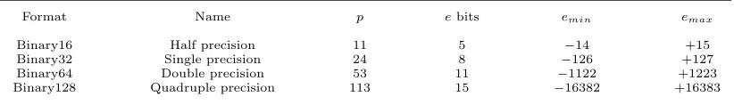
representations of the same number. The IEEE754 Standard also defines denormalized numbers which are floating-point numbers with d0 = d1 = . . . = dk = 0, k < p−1 and e = emin. Denormalized numbers make underflow gradual [7]. The IEEE754 Standard defines binary formats (with β = 2) and decimal formats (with β = 10). In this article, without loss of generality, we only consider normalized numbers and we always assume thatβ = 2 (which is the most common case in practice). The IEEE754 Standard also specifies a few values for p, emin andemaxwhich are summarized in Figure1. Finally, special values also are defined: nan (Not a Number) resulting from an invalid operation, ±∞corresponding to overflows, and +0 and−0 (signed zeros).
Format Name p ebits emin emax
Binary16 Half precision 11 5 −14 +15 Binary32 Single precision 24 8 −126 +127 Binary64 Double precision 53 11 −1122 +1223 Binary128 Quadruple precision 113 15 −16382 +16383
Figure 1: Basic binary IEEE754 formats.
The IEEE754 Standard also defines five rounding modes for elementary operations between floating-point numbers. These modes are towards −∞, towards +∞, towards zero, to the nearest ties to even and to the nearest ties to away and we write them↑−∞, ↑+∞,↑0,↑∼e and
↑∼a, respectively. The elementary operations ∈ {+, −, ×, ÷}are then defined by
f1 ↑◦ f2 =↑◦(f1 f2) (2)
where◦ ∈ {−∞,+∞,0,∼e,∼a}denotes the rounding mode. Equation (2) states that the result of a floating-point operation◦done with the rounding mode◦returns what we would obtain by
performing the exact operationand next rounding the result using◦. The IEEE754 Standard also specifies how the square root function must be rounded in a similar way to Equation (2) but does not specify the roundoff of other functions like sin, log, etc.
Because of the roundoff errors, the results of the computations are not exact. For example, the valuev= 2.7182818. . . can be computed using Bernoulli’s formula:
v= lim
n→+∞un with un=
1 + 1 n
n
, n≥0.
In double precision,u8= 2.718282 but then the accuracy decreases asngrows: u14= 2.716110,
u16 = 3.035035 and u17 = 1.0. The transformation techniques detailed in Section2.3 aim at
generating an expression which is mathematically equal to the original one and which minimizes the roundoff error on the result, i.e. the distance|r− ↑◦(r)|between the exact resultrand the
floating-point result↑◦(r). To deal with the errors introduced by the floating-point arithmetic,
we introduce the function↓◦:R→Rwhich computes the exact error due to rounding operation.
2.2
Error Bound Computation
In order to compute the errors during the evaluation of arithmetic expressions, we compute with values which are pairs (f, ε)∈F×R=Ewheref denotes the floating point number used by the machine and ε denotes the exact error ↓◦ (f) attached to f, i.e., the exact difference
between the real and floating-point numbers as defined in Equation (3). For example, the real number 1
3 is represented by the valuew= (↑∼ 1 3
,↓∼ 13) = (0.333333,(13−0.333333)). The
elementary operations onEis defined in [14].
In practice, we use a set based version of this arithmetic based on intervals. A so-called abstract value [5] is a pair of intervals such that the first interval corresponds to the range of the floating-point values of the program and the second interval corresponds to the range of the errors obtained by subtracting the floating-point values from the exact ones. In ([f],[ε])∈E], we have [f] the interval for the range of the values and [ε] the interval of errors on the values [f]. The pair ([f],[ε]) abstracts the set of concrete values {(f, ε) : f ∈ [f],and ε ∈[ε]} by intervals in a component-wise way.
We now introduce the arithmetic expressions on E]. We approximate an interval [x] with real bounds by an interval based on floating-point bounds, denoted by↑]◦([x]).
↑]
◦ ([x, x]) = [↑◦(x),↑◦(x)] . (4)
We denote by↓]◦ the function that abstracts the concrete function↓◦. It over-approximates
the set of exact values of the error ↓◦ (x) =x− ↑◦ (x). Every error associated to x∈[x, x] is
included in↓]◦([x, x]). We also have for the rounding mode to the nearest
↓]
◦([x, x]) = [−y, y] with y=
1
2ulp max(|x|,|x|)
. (5)
Formally, theunit in the last place, denoted byulp(x), is the weight of the least significant digit of the floating-point numberx. Equations (6) and (7) give the semantics of the addition and multiplication amongE], for other operations see [14]. If we sum two numbers, we must add errors on the operands to the error produced by the roundoff of the result. When multiplying two numbers, the semantics is given by the development of ([f]1+ [ε]1)×([f]2+ [ε]2).
([f]1,[ε]1) + ([f]2,[ε]2) = ↑]
◦([f]1+ [f]2),[ε]1+ [ε]2+↓
]
◦([f]1+ [f]2)
, (6)
([f]1,[ε]1)×([f]2,[ε]2) = ↑]◦([f]1×[f]2),[f]2×[ε]1+ [f]1×[ε]2+ [ε]1×[ε]2
+↓]◦([f]1×[f]2)
. (7)
2.3
Program Transformation for Numerical Accuracy
expressions:
A(p) =
(a+a) +b
×c, (a+b) +a
×c, (b+a) +a
×c,
(2×a) +b
×c, c× (a+a) +b
, c× (a+b) +a
, c× (b+a) +a
, c× (2×a) +b
, (a+a)×c+b×c,
(2×a)×c+b×c, b×c+ (a+a)×c, b×c+ (2×a)×c
(8)
To improve an expression, we first build its APEGA(p) and then we search inAthe most accurate expression following the error computation model of Section2.2.
2 a
× +
b □
+(a,a,b) ×
c ×
+
c b c ×
a a
+ ×
× +
Figure 2: APEG for the expression expr= (a+a) +b
×c.
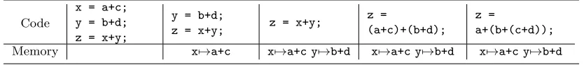
For commands, i.e. assignments, conditionals, loops, functions, etc., we use a set of transfor-mation rules allowing to mix the computations occurring in different instructions [6]. Basically, these rules build large expressions in order to offer more opportunities to rewrite them by asso-ciativity, commutativity, etc. For assignments, a first rule discards an assignment after saving it in the memory of the transformation tool and a second rule rewrites an assignment by inlin-ing the memorized expressions in the current expression, in order to build a larger expression. When the obtained expressions become too large, we slice them at a defined level of the syntac-tic tree and we assign the sub-expressions to intermediary variables. For example, let us take the code of Figure3 with three variablesx,yandzand constantsa= 0.1,b= 0.01,c= 0.001 andd= 0.0001. We aim at optimizingz.
Code
x = a+c; y = b+d; z = x+y;
y = b+d;
z = x+y; z = x+y;
z =
(a+c)+(b+d);
z =
a+(b+(c+d));
Memory x7→a+c x7→a+c y7→b+d x7→a+c y7→b+d x7→a+c y7→b+d
Figure 3: Example of code transformation.
We remove the variablexand memorize it. So, the first assignment is discarded and memo-rized. We then repeat the same process fory. We may not removezbecause it is the variable to be optimized. Then, we substitutexandyby their expressions and we transform the expression thanks to its APEG.
the last one seen in conditionals. At last, we use some rules dealing with sequences of commands and functions.
2.4
Code synthesis
Code synthesis is the mechanized construction of a program. Synthesizing tools takes a specifi-cation of what the program should do, then it automatically generates an implementation that provably satisfies this specification. Obviously, the synthesized code has to be as efficient as possible. In our context efficiently means numerically accurate and fast.
Synthesis Tool Linear Systems
+ Resolution method
Automatically Generated Implementation
Figure 4: Code Synthesis Process.
In our case, as a specifications, we consider a particular family of linear systems coming from the finite element discretization of a Mechanical system of PDE0s. The synthesizer tool should generate automatically a program for the numerical solvers applied on the specified linear system. Figure4illustrates the process of program synthesis.
3
The
Rock-N-Roll
tool
When we execute a numerical algorithm to solve a linear system of equations on a computer, each single operation introduces some roundoff errors, which are accumulated during the reso-lution process. Then, instead of the exact soreso-lutionxof a linear system we get an approximate result. In order to solve this accuracy problem, we have developed a code synthesis tool that generates automatically a fast and accurate C program for a given family of linear systems. In this section, we present this tool, Rock-N-Roll. We detail its architecture, its inputs and outputs.
3.1
Architecture
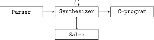
In this section, we describe the main architecture of our tool as shown in Figure5. Rock-N-Roll
is written inCand made of several modules, described hereafter:
Synthesizer
Parser C-program
Salsa
Figure 5: Software architecture of theRock-N-Rolltool.
matrix [A] = (aij])16i,j6n and the interval vector [b] = (bi])16i6n are build for each i andj as follows:
aij]= ([aij−aij×k1, aij+aij×k1],[−aij×k2, aij×k2]),
bi]= ([bi−bi×k1, bi+bi×k1],[−bi×k2, bi×k2]).
Wherek1 and k2 are two random (in our experiments Section 4, we gave k1 = 0.11 and
k2= 0.00001). Equation10describes an input family of linear :
[S] :
a11] · · · a1n] ..
. . .. an1] · · · ann]
x=
b1]
.. .
bn]
. (9)
Sinceaij]= ([f]ij ,[ε]ij) andbi]= ([f]i ,[ε]i) for all 16i6n and 16j 6n, we may rewrite Equation9 as:
([f]11 ,[ε]11) · · · ([f]1n ,[ε]1n) ..
. . ..
([f]n1 ,[ε]n1) · · · ([f]nn ,[ε]nn)
x=
([f]1 ,[ε]1) .. . .. . ([f]n ,[ε]n)
(10)
Recall from Section2.2that in the pairs ([f],[ε]), the first interval [f] consists of the range of floating-point value and the second interval [ε] consists of the error range associated to the floating-point interval [f].
• Salsa: It is a tool that improves the numerical accuracy of programs by automatic transformation, it takes a program as input and returns more accurate one [6]. The optimization done by Salsa depends on the ranges (intervals) given as inputs for the variables of the code to be optimized,
• Synthesizer: This module eliminates the zero elements of the given system. It produces a numerically optimized code for the Gaussian elimination rule for each abstract syntactic structure of aij] and bi]. In order to have more accurate results, theGaussSynthesis routine builds a specific code for theSalsa tool [6]. When theSalsa transformation is done, the synthesizer replaces the old piece of code by the transformed one, which is more accurate. In our case we have the choice between using the backward substitution, matrix inversion, LU-decomposition... etc.
• C-program: Rock-N-Roll outputs a file containing a C-program corresponding to the efficient implementation to compute an accurate solutionxofS∈[S] with the resolution method specialized for a given family of linear systems with much better accuracy.
4
Numerical experimentations
arising in Mechanics: The flexion of a beam fixed on its extremities and the compression of a viscoelastic body against a moving foundation. In both cases, the discretization is based on the finite element method (FEM) that was usually used to solve complicated problems in engineering, notably in elasticity and structural Mechanics modeling involving elliptic PDEs and complicated geometries. Note that the linear systems come from a Fortran computer code based on a MODULar Finite Element library (MODULEF)1. We compared between the
solu-tion namedxSGP M computed by synthesized Gauss pivoting method (SGPM) and the solution namedxCGP M calculated with a non-synthesized or what we named a classical Gauss pivoting method (CGPM).
4.1
Flexion of a beam
The first example consists of an academic but relevant mechanical problem which concerns the flexion of an 1D elastic beam with Dirichlet boundary conditions on its extremities where the physical setting is depicted in Figure6(for homogeneous Dirichlet boundary conditions).
α=0
β=0
f
u(x)
Figure 6: Physical setting of the flexion of a 1D beam.
To do that let us consider the following very simple 1D model problem which consist to find a displacementu∈C2([0,1],
R) such that,
(
−u00(x) =f ∀x∈]0,1[
u(0) =α and u(1) =β, (11)
where f is a constant vertical force acting on the domain interval Ω = [0,1]. In order to discretize the 1D elastic beam problem (11) and thus to obtain the related linear system, we use the finite element method. To do that, we have to introduce the mesh of the domain Ω = [0,1] by consideringN+ 1 nodes {xi, i = 1, .., N+ 1} of the interval [0,1] withx1 = 0,
xN+1 = 1 and xi+1 = xi +hi, for i = 1, .., N where h = max1≤i≤N{hi} is the mesh size. Therefore, the domain [0,1] is discretized into N nonuniform intervals (xi, xi+1) that are the
finite elements of sizehi. Then, we consider the simplest finite dimensional space that is to say the piecewise continuous linear function space defined over the mesh of the domain Ω = [0,1]. Thus, after elementary calculus (see [11] and [12]) we finally obtain the following tridiagonal systems, 1 h1 +C
−1 h1
−1 h1
1 h1+
1 h2 −1 h2 . .. . .. . .. −1 hN−1
1 hN−1 +
1 hN −1 hN 1 hN −1 hN +C
u1 u2 . . . uN uN+1 =f 2
h1+Cα
h1+h2 . . .
hN−1+hN
whereC is a large penalization value in order to take into account the boundary conditions at x= 0 and x= 1.
In such type of problem, it is well known that the previous linear system is ill-conditioned and the condition number of the matrix is related to themax1≤i≤N{h1i}. For this reason, it is an interesting example to test the Gauss Pivoting algorithm developed in Section3. For our experiment, we considered thatf =−20N/m2, max
1≤i≤N{h1 i}= 10
6, the penalization value
C= 106 and that the beam is fixed on its extremities (α=β = 0). First we created different
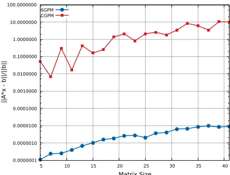
linear systems of size 4 6N 6 40. Then, we calculated the solution of each system by the synthesized Gauss pivoting (SGPM) program given by our toolRock-N-Roll: xSGP M and by a classical Gauss pivoting method (CGPM) program: xCGP M.
0.0000001 0.0000010 0.0000100 0.0001000 0.0010000 0.0100000 0.1000000 1.0000000 10.0000000 100.0000000
5 10 15 20 25 30 35 40
||
A
*x
b
||
/|
|b
||
Matrix Size
SGPM CGPM
Figure 7: Comportment of the relative errors of the solutions for different sizes.
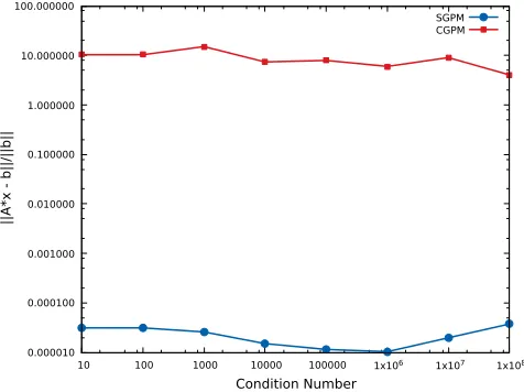
Finally, in order to highlight the differences between solutions, we compute and display in
Figures7and8the relative errorRelErr(x) = kA∗x−bk2
kbk2
of each solution ones with
increas-ing the condition number and keepincreas-ing the size constant and conversely. We can observe a sig-nificant difference between the curves corresponding toRelErr(xSGP M) andRelErr(xCGP M), which are calculated with xSGP M and xCGP M respectively. We see that the difference in accuracy between the results of the two methods is of the order of 5×10⁻⁶on average.
We can also see that the increase of the error is more regular and smoother with the solution calculated by the program generated byRock-N-Rollin both of the condition number and the matrix size figures.
For execution time measurements, all the programs have been written in the C language and compiled withGCC 4.9.2-03, and executed onIntel Core i7in IEEE754 single precision in order to emphasize the effect of the finite precision. The results displayed in Figure9show that by synthesizing Gauss pivoting code, we improve not only its accuracy but we reduce its execution time too. This is mainly due to the fact that the systems comingfrom from our mechanical problem are sparse and that is the case,Rock-N-Roll is able to simplify the computation and to remove all the zero terms. For instance, in the examples of Section??some zero terms have been removed in the expression ofx2andB4otherwise we would have a far more
0.000010 0.000100 0.001000 0.010000 0.100000 1.000000 10.000000 100.000000
10 100 1000 10000 100000 1x10⁶ 1x10⁷ 1x10⁸
||
A
*x
b
||
/|
|b
||
Condition Number
SGPM CGPM
Figure 8: Comportment of the relative errors of the solutions for different condition numbers.
0.1 0.2 0.3 0.4 0.5 0.6 0.7 0.8 0.9
5 10 15 20 25 30 35 40
T
im
e
/s
Matrix Size
SGPM CGPM
Figure 9: Execution time measurements of SGPM-program generated byRNRand CGPM-program
4.2
A frictional contact problem with a moving foundation
example, it is obvious that other methods of resolution (as preconditioned gradient conjugate for instance) can be used to solve such kind of systems. In this problem, the ill-conditioning comes from the frictional contact conditions that leads to large terms in the linearized systems related to the numerical treatment (augmented Lagrangian method and penalization method) of these non-smooth and non linear boundary conditions.
Ωdeformable body
Γ1
f2
Γ3 contact interface
x2
x1
0000000000000000000000000000000
1111111111111111111111111111111
0000000000000000000000000000000 0000000000000000000000000000000 0000000000000000000000000000000 0000000000000000000000000000000 0000000000000000000000000000000 0000000000000000000000000000000 0000000000000000000000000000000 0000000000000000000000000000000 0000000000000000000000000000000
1111111111111111111111111111111 1111111111111111111111111111111 1111111111111111111111111111111 1111111111111111111111111111111 1111111111111111111111111111111 1111111111111111111111111111111 1111111111111111111111111111111 1111111111111111111111111111111 1111111111111111111111111111111
Γ2
g
v*
crust
moving foundation
asperities
rigid material
Figure 10: Physical setting of the sliding frictional contact problem.
moving foundation v*
v*
moving foundation
Figure 11: Deformed meshes with respect to two opposite velocity of the moving foundation.
The physical setting used for this problem is depicted in Figure10. Here, we consider the frictional contact between a deformable body and a moving foundation. This specific foundation is composed by a rigid material covered by a thin crust and a deformable layer of asperities of depth g. Here g represents the maximum value of the allowed penetration in the foundation. When this value of penetration is reached, the contact follows a unilateral condition without any additional penetration. Since the foundation is moving, the friction condition is in a slip status within the Coulomb’s form. The deformable body is a rectangle, Ω = (0,2)×(0,1)⊂R2, and its boundary Γ is split as follows: Γ1= ({0} ×[0,1]), Γ2= ((0,2)× {1})∪({2} ×[0,1)),
Γ3 = (0,2]× {0}. The domain Ω represents the cross section of a three-dimensional linearly
viscoelastic body subjected to the action of tractions in such a way that a plane stress hypothesis is assumed. On the part Γ1the body is clamped and, therefore, the displacement field vanishes
there. Vertical compressions act on the part (0,2)× {1} of the boundary Γ2 and the part
body. The body is in frictional contact with an obstacle on the part Γ3 of the boundary. For
the numerical simulations, all the data concerning the problem can be found in [4].
In Figure 11, we present the two deformed configurations of the body with respect to two opposite velocity of the moving foundation.
For this second example, in order to illustrate the efficiency of the Rock-N-Roll tool we consider the first linearized system generated during the last iteration of the Newton solver. This linear system has the particularity to be non-symmetric due to the presence of friction terms, and ill-conditioned because of the augmented Lagrangian approach for the treatment of frictional contact conditions. (see [1,4, 9,13]).
0.0000001 0.0000010 0.0000100 0.0001000 0.0010000 0.0100000 0.1000000 1.0000000 10.0000000
10 100 1000
||
A
*x
b
||
/|
|b
||
Matrix Size
SGPM CGPM
Figure 12: Comportment of the relative errors of the solutions for different sizes.
0 0.1 0.2 0.3 0.4 0.5 0.6 0.7 0.8
10 100 1000
T
im
e
i
n
S
e
co
n
d
s
Matrix Size
SGPM CGPM
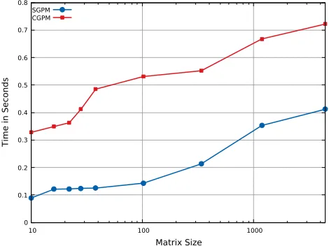
Figure 13: Execution time measurements of SGPM-program generated byRNRand CGPM-program
displayed, both for the CGPM-program and SGPM-program generated by our Rock-N-Roll
tool with respect to 9 different sizes. As for the first example, a significant difference between the two methods is observed in favor of Rock-N-Roll. In Figure12, we see that the difference in accuracy is of order 10−2. The results displayed in Figure13show that the SGPM-program
generated byRock-N-Roll is faster. We can see a 30% increase (for the resolution time) for the CGPM whereas this increase is only 2% for the SGPM-program time implemented by our synthesizerRock-N-Roll.
5
Conclusion
In this article, we have introduced a synthesized Gauss pivoting method implemented in
Rock-N-Roll, an automatic synthesizer tool to improve the numerical accuracy of linear systems resolution, specifically systems coming from mechanical problems. We have detailed its architec-ture, and the different inputs and the outputs that it supports. We have testedRock-N-Roll
across experimental results obtained on two examples coming from two different mechanical problems with and without contact. The results obtained show the efficiency of our synthesized Gauss pivoting method which improves the numerical accuracy of computations compared to the classical Gauss pivoting method, so as the execution time. An interesting perspective con-sists of extending our work to synthesize Gauss pivoting method on partitioned matrices and also parallel. Furthermore, as prospect it would be interesting to add the Conjugated Gradient and the double Conjugated Gradient methods to ourRock-N-Roll. Taking into account non linear solvers as Newton type methods would be very challenging in the framework of numerical accuracy.
References
[1] P. Alart and A. Curnier, A mixed formulation for frictional contact problems prone to Newton like solution methods,Comput. Meth. Appl. Mech., Engrg.92, 353-375, 1991.
[2] ANSI/IEEE. IEEE Standard for Binary Floating-point Arithmetic. ANSI/IEEE, std 754-2008 edition, 2008.
[3] Atkinson, Kendell A. An introduction to numerical analysis (2nd ed.). John Wiley and Sons. ISBN 0-471-50023-2, 1998.
[4] M. Barboteu & Y. Souleiman, Numerical Analysis of a Sliding frictional contact problem with Normal Compliance and Unilateral Contact, submitted toMathematical Methods in the Applied Sciences, Wiley.
[5] P. Cousot and R. Cousot. Abstract interpretation: a unified lattice model for static analysis of programs by construction or approximation of fixpoints. InPrinciples of Programming Languages, pages 238–252. ACM Press, 1977.
[6] N. Damouche, M. Martel, and A. Chapoutot. Intra-procedural optimization of the numerical accuracy of programs. InFMICS’15, volume 9128 ofLNCS, pages 31–46. Springer, 2015. [7] D. Goldberg. What every computer scientist should know about floating-point arithmetic. ACM
Computing Surveys, 23(1), Mar, 1991.
[8] Grossmann, Christian, Roos, Hans-G., Stynes, Martin. Numerical Treatment of Partial Differential Equations. Springer. ISBN 978-3-540-71584-9, 2007.
[10] A. Ioualalen and M. Martel. A new abstract domain for the representation of mathematically equivalent expressions. InSAS’12, volume 7460 ofLNCS, pages 75–93. Springer, 2012.
[11] T. JR. Hughes,The finite element method, Prentice Hall, 1987. [12] N. Kikuchi,Finite element methods in Mechanics, Cambridge, 1986.
[13] T. Laursen,Computational Contact and Impact Mechanics, Springer, Berlin, 2002.
[14] M. Martel. Semantics of roundoff error propagation in finite precision calculations. Higher-Order and Symbolic Computation, 19(1):7–30, 2006.
[15] Panchekha, P., Sanchez-Stern, A., Wilcox, J.R., Tatlock, Z.: Automatically improving accuracy for floating point expressions. In: PLDI. pp. 1–11. ACM, 2015.
[16] Saad, Yousef. Iterative methods for sparse linear systems (2nd ed.). Philadelphia, Pa.: Society for Industrial and Applied Mathematics. p. 195. ISBN 978-0-89871-534-7, 2003.
[17] M. Sofonea and A. Matei, Mathematical Models in Contact Mechanics, London Mathematical Society Lecture Note Series398, Cambridge University Press, Cambridge, 2012.
[18] M. Sofonea & Y. Souleiman, A Viscoelastic Sliding Contact Problem with Normal Compliance, Unilateral Constraint and Memory Term,Mediterranean Journal of Mathematics.13, 2863–2886, 2016.