Numerical Method For Approximate Solutions of Fractional Differential Equations with Time Delay

(1)

Vol. 3, No. 2, pp. 127-136, April (2020)

Numerical Method for Approximate Solutions of

Fractional Differential Equations with

Time-Delay

Fahimeh Akhavan Ghassabzadeh

1

, Samaneh Soradi-Zeid

2,†

1_{Department of Mathematics, Faculty of Sciences, University of Gonabad, Gonabad, Iran} 2_{Faculty of Industry and Mining (Khash), University of Sistan and Baluchestan, Zahedan, Iran.}

Due to the easy adaption of radial basis functions (RBFs), a direct RBF collocation method is considered to develop an approximate scheme to solve fractional delay differential equations (FDDEs). In spite of easy implementation of other high-order methods and finite difference schemes for solving a problem of fractional order derivatives, the challenge of these methods is their limited accuracy, locality, complexity and high cost of computing in discretization of the fractional terms, which suggest that global scheme such as RBFs that are more accurate way for discretizing fractional calculus and would allow us to remove the ill-conditioning of the system of discrete equations. So, the proposed approach, either employ any global RBFs for interpolating technique or uses arbitrary points for discretization, offers a very flexible framework for solving FDDEs. Applications to a variety of problems confirm that the proposed method is slightly more efficient than those introduced in other literatures and the convergence rate of our approach is high.

Article Info

Keywords:

Collocation method, Direct method, Error analysis, Fractional delay differential equation, Radial basis function. Article History:

Received 2019-05-30

Accepted 2020-01-19

I.

I

NTRODUCTION

Using fractional order dynamics for diaphragms, bellows, and other devices that may have sprig-property yields a more accurate model for such industrial systems than the classical integer order models. In particular, relaxation processes deviating from the classical exponential behavior are often encountered in the dynamics of complex materials. In recent decay, the applications of fractional calculus in scientific fields such as power and environment sciences is improved and this has caused that the FDDEs have been review by many researchers due to their applications over the simulation and modeled in engineering, physics, hydrology, pure and applied mathematics [1, 2, 3, 4]. Many considerable studies on the theory, existence of solutions and numerical analysis of FDDEs have been presented in [5, 6, 7, 8, 9, 10]. Dehghan

et al. used the concept of Legendre operational matrix to present the numerical solutions of FDDEs in [11]. Morgado [12], applied the Mittag-Leffler functions to approximate solutions for FDDEs. The Chebyshev wavelet method to compute an approximation to the solution of the FDDEs has been employed in [13]. Dehghan et al. [14] used the variational iteration and Adomian decomposition methods to obtain the approximate solutions for the delay logistic equation. Amar et al. in [15], concentrated on developing an efficient approximate solution of fractional delay quasi-linear control inclusion. Finite difference scheme is applied to solve the FDDEs in [16]. Wang [17] approximated the FDDEs by combining the general Adams-Bashforth-Moulton method with the linear interpolation method. In another paper, Wang et al. [18] introduced a numerical method for nonlinear functional order differential equations with constant time varying delay, based on Grunwald-Letnikov definition. Recently, Pandey et al. [19] applied the Bernstein’s

†_{Corresponding Author:}_{[email protected]}

Tel: +98-54-33723560, University of Sistan and Baluchestan, Faculty of Industry and Mining (Khash), Zahedan, Iran.

(2)

International Journal of Industrial Electronics, Control and Optimization .

…

128

operational matrix for the fractional derivative to solve two FDDEs of physical importance. Mohammadi in [20] used Chelyshkov-Wavelet to solve systems of FDDEs and a finite time stability results for FDDEs by virtue of delayed Mittag-Leffler type matrix present in [21]. The review article [22] contains an up-to-date bibliography on numerical methods for solving FDDEs.

The field of industry is a special application domain for fractional order systems as the demanding performance expectations with uncertainties make it a challenge to come up with models that are useful, or control modules that can alleviate the difficulties in various forms. The interest of the industry to fractional order systems lie in the fact that complicated modules can be simplified significantly and practical applications can be diverse. The investigation of industrial mathematics problems sometimes leads to the development of new methods of solution of differential equations. This special issue has covered both the theoretical and applied aspects of industrial mathematics. Papers contain the development of new mathematical models or well-known models applied to new physical situations as well as the development of new mathematical techniques [23, 24, 25, 26, 27]. This is bilaterally meaningful collaboration between mathematics and industry. Some literatures [28, 29, 30] consider the fractional order systems and control methods (such as PID controller, adaptive control and sliding mode control) within the context of industrial automation. The expectations of the industrial applications are demanding and often times the conventional solutions to problems are so complicated that the manufacturing of the goods based on standard approaches is not feasible. To overcome this challenge, we present a practical direct numerical method to solve these equations.

Radial basis techniques are one of the relatively new techniques used for finding solutions of fractional differential equations (FDEs). Due to better accuracy, stability, efficiency, memory requirement, and simplicity of implementation of RBFs over other methods, a number of researchers are being attracted toward these techniques. RBF meshless method used by Liu et al. in [31] for solving time fractional advection-diffusion equation with distributed order and by Dehghan et al. in [32] for solving the nonlinear time fractional Sine-Gordon and Klein-Gordon equations. Ahmadi et. al. applied RBFs for solving stochastic fractional differential equations in [33]. In addition, the local RBF method has been investigated in [34] to solve the variable-order time fractional diffusion equation. Also, RBFs are actively used for solving KdV equation in [35, 36]. A local RBFs collocation method based on the MQ RBFs for solving nonlinear coupled Burgers equations is presented in [37]. Kumar and Yadav in [38] provide RBF neural network techniques for solving differential equations of various kinds. Some other work related to this field may be found in [39, 40,

41]. Control systems can include both the fractional-order dynamic system to be controlled and the fractional-order controller. However, in the current paper, we focus on providing a numerical scheme based on RBFs to solve the following FDDE:

𝐷𝛼_{𝑥(𝑡) = 𝑎(𝑡)𝑥(𝑡) + 𝑏(𝑡)𝑥(𝑡 − 𝜏) + 𝑓(𝑡),} 𝑡𝜖(0, 𝑇], 𝜏 > 0, 𝑛 − 1 < 𝛼 ≤ 𝑛

𝑥(𝑡) = 𝜑(𝑡), − 𝜏 ≤ 𝑡 ≤ 0. (1) where 𝑎, 𝑏 and 𝑓 are continuous functions on [0, 𝑇], the initial function 𝜑 is a continuous function on [−𝜏, 0] and 𝐷𝛼_{denotes the Caputo derivative of order} _𝛼_{that was} defined as follow:

Definition 1. The Caputo fractional derivative of order α is defined by

𝐷𝛼_{𝑓(𝑡) =} 1

Γ(𝑛 − 𝛼)∫(𝑡 − 𝜏)𝑛−𝛼−1𝑓(𝑛)(𝜏)𝑑𝜏 𝑡

𝑡₀

,

𝑛 − 1 < 𝛼 ≤ 𝑛, 𝑡 > 0, (2)

where Γ(. ) is a Gamma function and 𝐷𝛼 satisfies the following properties:

𝐷𝛼_{𝐾 = 0 (𝐾 𝑖𝑠 𝑎 𝑐𝑜𝑛𝑠𝑡𝑎𝑛𝑡),} 𝐷𝛼_𝑥𝛽₌ Γ(𝛽+1)

Γ(𝛽−𝛼+1)𝑥

𝛽−𝛼_{, 𝛽 > 𝛼 − 1 (𝑤ℎ𝑒𝑛 𝑡}

0= 0 𝑖𝑛 (2)) 𝐷𝛼_{(𝜆𝑓(𝑡) + 𝜇𝑔(𝑡)) = 𝜆𝐷}𝛼_{𝑓(𝑡) + 𝜇𝐷}𝛼_{𝑔(𝑡). (3)}

(3)

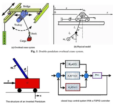
Fig. 1: Double-pendulum overhead crane system.

Fig. 2: Closed loop control system With a PID controller.

II. RBF CALLOCATION METHOD FOR

SOLVING FDDEs AND ERROR ESTIMATE

The industrial applications exploiting the expertise of systems and control engineering has a significantly wide spectrum covering the open-loop characterization of processes to develop high-performance feedback mechanisms, tuning of controllers via expert knowledge and computer tools, adaptive and selftuning mechanisms taking care of the changes in the process dynamics, nonlinear, robust and optimal control policies to meet a predefined set of performance criteria, fault tolerant schemes, and safety critical applications. The ultimate expectation in all such branches of industry is to maintain the production, while keeping the cost at minimum possible level.

Looking at the sectors and their needs, in the sequel, we propose a numerical computational approach based on RBF collocation method to directly solve the FDDEs. At first, we introduced and utilized the RBFs to interpolate a function in any dimensions. A function 𝜙: ℝ𝑑→ ℝ is called to be radial if there exists a univariate function 𝜑: [0, ∞) → ℝ such that

𝜙(𝑥) = 𝜑(𝑟), where 𝑟 =∥ 𝑥 ∥ and ∥. ∥ is usually Euclidean distance on ℝ𝑑, although other distance functions are also possible.

Definition 2 Commonly used types of RBFs include the following forms in which 𝑟 =∥ 𝑥 − 𝑥𝑖 ∥ and the shape parameter 𝜀 controls their flatness [45, 46]:

- Piecewise Smooth:

𝜙(𝑟) = 𝑟3, Cubic RBF 𝜙(𝑟) = 𝑟5, Quintic RBF

𝜙(𝑟) = 𝑟2𝑙𝑜𝑔(𝑟), Thin Plate spline (TPS) RBF 𝜙(𝑟) = (1 − 𝑟)𝑚+ 𝑝(𝑟), Wendland functions where 𝑝 is a polynomial.

- Infinitely Smooth:

𝜙(𝑟) = √1 + (𝜀𝑟)2, Multiquadric (MQ) RBF

𝜙(𝑟) =_1+(𝜀𝑟)1 ₂, Inverse Quadratic (IQ) RBF

𝜙(𝑟) = 𝑒−(𝜀𝑟)2, Gaussian RBF. Next, we proceed by discussing on RBFs approximation. Definition 3 Given a global radial function 𝜙(𝑟), 𝑟 ≥ 0, scattered points 𝑥1, 𝑥2, ⋯ , 𝑥𝑁 selected on the domain 𝛺 ⊂ ℝ𝑑_{and data}_𝑓

(4)

International Journal of Industrial Electronics, Control and Optimization .

…

130

interpolating RBF approximation for function 𝑠(𝑥) at an arbitrary point 𝑥 ∈ 𝛺 takes the form:

𝑠(𝑥) = ∑ 𝑁

𝑖=1

𝜆𝑖𝜙(∥ 𝑥 − 𝑥𝑖 ∥) + 𝜓(𝑥), (4)

where 𝜆𝑖 are the set of unknown RBF coefficients to be determined by the interpolation conditions 𝑠(𝑥𝑖) = 𝑓𝑖, 𝑖 = 1,2, ⋯ , 𝑁 and 𝜓 is a polynomial. The input variable 𝑥 and points 𝑥𝑖 can be either scalars or vectors. As well, in a similar representation as Eq. (4), for any linear fractional differential operator 𝐷𝛼, 𝐷𝛼𝑠(𝑥) can be approximated by:

𝐷𝛼_{𝑠(𝑥) = ∑} 𝑁

𝑖=1

𝜆𝑖𝐷𝛼𝜙(∥ 𝑥 − 𝑥𝑖 ∥) + 𝐷𝛼𝜓(𝑥) ₍₅₎

Eq. (4) can be written without the additional polynomial 𝜓. In that case, 𝜙 must be strictly positive definite to guarantee the solvability of the resulting system (e.g., Gaussian or inverse multiquadrics). However, 𝜓 is usually required when 𝜙 is conditionally positive definite, i.e., when 𝜙 has a polynomial growth toward infinity [46, 47]. Obtaining a closed form analytic expression for the fractional derivative of a radial function may lead to a challenge. Accordingly, Mohammadi and Schaback in [48], provide the required formulas for the fractional derivatives of RBFs in which allow us to use high order numerical methods for solving fractional problems such as FDDEs.

Now, we briefly introduce the RBFs collocation method. Consider the following boundary value problem when Ω ⊂ ℝ𝑑_:

𝐿𝑢 = 𝑓 𝑖𝑛 Ω (6) 𝑢 = 𝑔 𝑜𝑛 𝜕Ω (7) where 𝐿 is a linear differential operator and 𝑑 is the dimension of the problem. We distinguish in our notation centers of RBFs 𝑋 = {𝑥1, . . . , 𝑥𝑁} and the collocation points Ξ = {𝛼1, . . . , 𝛼𝑁}. Then we have the approximate solution of (2.3) and (2.4) in the form:

𝑢̃(𝑥) = ∑𝑁

𝑖=1𝜆𝑖𝜙(∥ 𝑥 − 𝑥𝑖 ∥), (8) where 𝜆𝑖, 𝑖 = 1,2, ⋯ , 𝑁, are unknown coefficients that

determined by collocation, 𝜙 is a RBF, ∥. ∥ is the Euclidean norm and 𝑥𝑖 is the centers of the RBFs.

Now, let Ξ divided into two subsets. One subset contains 𝑁𝐼 centers, Ξ1, where Eq. (6) is enforced and the other subset contains 𝑁𝐵 centers, Ξ2, where boundary conditions are enforced. The collocation matrix that is obtained by matching the differential equation and the boundary condition at the collocation points has the following form:

, I B A A A  _{ }  

in which, 𝐴𝐼= 𝐿𝜙(∥ 𝛼 − 𝑥𝑗∥)𝛼=𝛼_𝑖,𝛼𝑖∈ Ξ1,𝑥𝑗∈ 𝑋, and

𝐴𝐵= 𝐿𝜙(∥ 𝛼 − 𝑥𝑗∥)𝛼=𝛼_𝑖, 𝛼𝑖∈ Ξ2, 𝑥𝑗∈ 𝑋. The unknown coefficients 𝜆𝑖 are determined by solving the linear system 𝐴𝜆 = 𝐹, where 𝐹 is a vector included 𝑓(𝛼𝑖), 𝛼𝑖 ∈ Ξ1, and 𝑔(𝛼𝑖), 𝛼𝑖 ∈ Ξ2.

A. APPLICATION OF RBF COLLOCATION METHOD In this section, we will develop the RBF collocation method for solving problem (1). For this purpose, we rewrite problem (1) as the following form:

        



 

1 ; 0 ,

0, 0,

D u t a t u t b t u t f t t T

u t t

 _



     

    (9)

where 𝑢(𝑡) = 𝑥(𝑡) − 𝑤(𝑡) is a new unknown function that

𝑤(𝑡) = {𝜑(𝑡), 𝑡 ∈ [−𝜏, 0] 0, 𝑡 ∈ (0, 𝑇] and

𝑓1(𝑡) = {𝑓(𝑡) + 𝑏(𝑡)𝜑(𝑡 − 𝜏), 𝑡 ∈ [0, 𝜏]_{𝑓(𝑡), 𝑡 ∈ (𝜏, 𝑇].}

The unknown functions 𝑢(𝑡) and 𝑢(𝑡 − 𝜏) are approximated using 𝑁 RBFs as following:

𝑢(𝑡) ≃ ∑𝑁

𝑖=1𝜆𝑖𝜙(∥ 𝑡 − 𝑡𝑖 ∥) = ∑𝑁

𝑖=1𝜆𝑖𝜙𝑖(𝑡) (10)

(11) 𝑢(𝑡 − 𝜏) ≃ ∑

𝑁

𝑖=1

𝜆𝑖𝜙(∥ 𝑡 − 𝜏 − 𝑡𝑖∥)

= {

0, 0 ≤ 𝑡 ≤ 𝜏

∑ 𝑁

𝑖=1

𝜆𝑖𝜙𝑖(𝑡 − 𝜏), 𝜏 ≤ 𝑡 ≤ 𝑇.

By substituting (10)-(11) in (9), we have:

   





 

1 1 1 1 1

; 0 , 0, 0,

N N

i i i i i i

i i i N i N i i

D t a t t b t t f t t T

t t                      



(12) Rewrite (12) for collocation nodes {𝑡𝑘}𝑘=1𝑁 , yields a system of 𝑁 linear equations with 𝑁 unknowns as follow:

        







 

1 1 1

; 0

0, 0. N i i N i i

i k k i k k i k k k

i k k

D t a t t b t t f t t

t t _ _ _ _               



(13) One can write this system in matrix form as:

0 Λ= , A F B            (14)

(5)

with elements

𝐵𝑖𝑗= 𝐷𝛼𝜙𝑗(𝑡𝑖+1) − 𝑎(𝑡𝑖+1)𝜙𝑗(𝑡𝑖+1) − 𝑏(𝑡𝑖+1)𝜙𝑗(𝑡𝑖+1− 𝜏) furthermore, Λ ∈ ℝ𝑁 is the vector of unknown coefficients and the components of 𝐹 are the data 𝑓1(𝑡𝑗), 𝑗 = 2,3, ⋯ , 𝑁.

Finally, by solving the above system of algebraic equations, we can find the unknown coefficients {𝜆𝑖}𝑖=1𝑁 . Consequently 𝑢(𝑡) can be approximated by (10) and 𝑥(𝑡) is approximated from 𝑥(𝑡) = 𝑢(𝑡) + 𝑤(𝑡).

B. Error estimate

In this section, the error analysis of the applied method for solving FDDEs will be provided. Exponential convergence estimates for the RBFs interpolation provided from [46]. For simplicity, in the next, we will assume that Ω = [0,1]. In this position for subsequent error analysis, we have to consider the following definition and theorems.

Definition 4 A real-valued continuous even function 𝜙 is called positive definite on 𝛺 if

∑𝑁

𝑗=1∑𝑁𝑘=1𝑐𝑗𝑐𝑘𝜙(𝑥𝑗− 𝑥𝑘) ≥ 0, (15) for different points 𝑥1, 𝑥2, ⋯ , 𝑥𝑁∈ Ω , and 𝑐 = [𝑐1, 𝑐2, ⋯ , 𝑐𝑁]𝑇∈ ℝ𝑁. The function 𝜙 is called strictly positive definite on Ω if the only vector 𝑐 = 0 that turns (2.12) into an equality is the zero vector [46].

Theorem 1 [46] Suppose that 𝜙 is positive definite RBF with infinite smoothness. Let 𝑠(𝑥) be the interpolate to 𝑓 by using RBF approximation 𝜙 in (4). Then, there is a positive constant 𝐶, independent of 𝑋, such that

∥ 𝑓(𝑥) − 𝑠(𝑥) ∥∞≤ 𝐶ℎ𝑋|𝑓(𝑥)|ℵ_𝜙(Ω), 𝑥 ∈ Ω, (16) where ℵ𝜙(Ω) is the so called real native Hilbert space of 𝜙

on Ω (the idea of the native spaces introduced in [49]) and ℎ𝑋= sup

𝑥∈Ωmin𝑥𝑖∈𝑋∥ 𝑥 − 𝑥𝑖∥, (17)

is the fill distance of a set of points 𝑋 = {𝑥1, 𝑥2, ⋯ , 𝑥𝑁} on Ω.

Therefore, the infinitely smooth RBFs such as Gaussians and (inverse) multiquadrics have a high convergence rates for local interpolation RBFs [49]. As a result of Theorem 1, the error for the RBF interpolation of delay function in (1) is similar to (16) and for the fractional derivative of 𝑓 ∈ ℵ𝜙(Ω) ∩ 𝑊∞𝑚(Ω) defined by (5) we have [50]:

 

2 

 

  1

, Ω Ω

Ω

sup |_{m L} | ,

x

D f x D s x CN f x f x

           _  _   (18) where, 𝜙 is strictly positive definite and 𝑊∞𝑚 is the Sobolev space.

Let us suppose that 𝐸(𝑡) = 𝑢(𝑡) − 𝑢̂(𝑡) is the error function where 𝑢(𝑡) is the exact solution of the FDE (9) and 𝑢̂(𝑡) is that the approximate solution of this equation that is given by Eq. (10) . Therefore,

        



 

1 1

2

; 0 , , 0.

ˆ ˆ ˆ

ˆ

D u t a t u t b t u t f t R t t T

u t R t t

 _



      

   

(19) Now, by subtracting (9) from (19), we have:



   





 

   

2

 

1

;

, 0.

ˆ ˆ ˆ

ˆ

D u u t a t u u t b t u u t R t

u t u t R t t

 _



       

     

(20) Now, the error function 𝐸(𝑡) is established by the following equation:

        



 

1

2

; 0 ,

, 0,

D E t a t E t b t E t R t t T

E t R t t

 _



      

    

(21) in which, 𝑅1(𝑡) and 𝑅2(𝑡) are known functions in the collocation points. So, to find approximate error, we can follow the same method mentioned in the last section.

III.

RESULT

AND

DISCUSSIONS

In this section, we use the presented numerical approach to solve two illustrative examples. Based on the pervious discussion, as 𝑁 → ∞, the error of the RBF interpolation is bounded. So, the convergence behavior of the method is confirmed by some numerical examples in this section. All the computations were carried out using the Matlab software. Here, we will consider the power RBF as 𝜙(𝑟) = 𝑟𝑛 with 𝑛 = 3. Here, the error between the exact solution 𝑥(𝑡) and the approximate solution 𝑥̃(𝑡) , found using our method, namely the absolute error and computed as follows:

𝐸𝑟𝑟𝑜𝑟{𝑥(𝑡), 𝑥̃(𝑡)} =∥ 𝑥(𝑡) − 𝑥̃(𝑡) ∥∞,

𝑡 ∈ [0, 𝑇] (22)

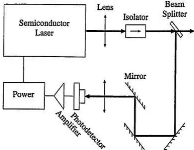
Example 1 As an applicable problem, we consider the problem of the effect of noise on light which is reflected from laser to mirror as follows:

𝐷𝛼_{𝑥(𝑡) =}−1 𝜖 𝑥(𝑡) +

1

𝜖𝑥(𝑡)𝑥(𝑡 − 1), 0 < 𝛼 ≤ 1, 𝑡 > 0, 𝑥(𝑡) = 0.9, −1 ≤ 𝑡 ≤ 0.

(6)

International Journal of Industrial Electronics, Control and Optimization .

…

132

Fig. 3: Semiconductor laser subject to an optoelectronic feedback.

Fig.4: The numerical solution of Example (1) at different values of 𝛼 with 𝜖 = 0.1 and 𝑁 = 20.

Example 2 Consider the following FDDE:

  

  

 





1 3

2 2

2

Γ 3

1 2 1 , 0

5 Γ

2

, 1,0 .

D x t x t x t t t t

x t t t

      

     

  

The exact solution in this case is 𝑥(𝑡) = 𝑡2 for 𝑡 ≥ 0. This problem was introduced by Morgado et. al. [12] in which the authors analyzed existence and uniqueness solutions for initial value problems of linear FDDEs. The authors in [5] used the shifted Jacobi polynomials for solving this problem. The method based on reproducing kernel space for approximated solution of this problem obtained by [50]. In Fig. 5, we plotted the exact solution and the approximated solution of 𝑥(𝑡) for 𝑁 = 15,25,30. As expected, we can observe by increasing the value of 𝑁, the approximated solution converge to the exact values. The absolute errors of the presented method for this example, shown in Fig. 6 and

Fig. 7. To evaluate the efficiency and performance of the RBF collocation method presented in Section 2 is better than those introduced in other literatures, a comparison is made between the absolute errors obtained by our method for different values of 𝑁 with the best results that achieved by other researchers in Table 1. From the perspective of this table, our suggested approach is somewhat more effective by increasing 𝑁.

Example 3 Consider the following FDDE:

  

  

 





2.7

0.3 2

3

2000

1 1 3 3

1071Γ 0.7

, 1,0 ,

t D x t x t x t t t

x t t t

      

  

The exact solution in this case is 𝑥(𝑡) = 𝑡3 for 𝑡 ≥ 0. The absolute errors of the presented method for this example, shown in Fig. 8. Also, Table 2, demonstrates the effect of various values of 𝑁 for this example. Comparing the numerical results obtained in this table, reveals that the accuracy of the RBF collocation method is higher than the methods presented in [12, 52].

Table I: Absolute errors and CPU time(second) at different choices of N in [0,100] for Example (2).

𝑵 Ref. [12] This study CPU time

𝟏𝟎𝟎𝟎 0.0491843 0.0785 1.864828

𝟐𝟎𝟎𝟎 0.0276172 0.0221 7.398307

𝟒𝟎𝟎𝟎 0.0146507 0.0063 30.177423

𝟖𝟎𝟎𝟎 0.0075649 0.0018 129.507482

III.

C

ONCLUSIONS

(7)

Fig. 5: Exact and approximate values of 𝑥(𝑡) at different values of 𝑁 in [0,2] for Example (2).

Fig. 6: Absolute error of x(t) with N = 500 in [0,2] for Example (2).

Fig. 7: Absolute error of x(t) with N = 4000 in [0,100] for Example (2).

Table II:Absolute error and CPU time (second) at different choices of N in [0,100] for Example (3).

𝑁 Ref. [12] Ref. [52] This study CPU time

1000 0.0710508 0.00001 3.0268𝑒 − 09 1.855609

2000 0.0411543 − − 6.4028𝑒 − 09 7.475098

4000 0.0219612 − − 1.7899𝑒 − 08 31.21183

8000 0.0113125 − − 2.5844𝑒 − 08 132.473657

(8)

International Journal of Industrial Electronics, Control and Optimization .

…

134

Fig. 8: Absolute error of x(t) with N = 500 in [0,10] for example (3).

R

EFERENCES

[1] H. L. Smith, “An introduction to delay differential equations with applications to the life sciences,” Vol. 57, New York, Springer. 2011.

[2] G.A. Walter, H.I. Freedman, J. Wu , “Analysis of a model representing stage-structured population growth with state-dependent time delay,” SIAM Journal Appl Math, Vol.52, No.3,: pp. 855-869 , 1992.

[3] Y. Kuang, “Delay differential equations: with applications in population dynamics”, Academic Press, New York, 1993. [4] M. Malek-Zavarei, M .Jamshidi, “Time-delay systems:

analysis optimization and applications”, Elsevier Science Ltd, New York, 1987.

[5] P. Muthukumar, and B. Ganesh Priya, “Numerical solution of fractional delay differential equation by shifted Jacobi polynomials,” International Journal of Computer Mathematics, Vol. 94, No. 3, pp.471-492, 2017. [6] V. Daftardar-Gejji, Y.Sukale, and S. Bhalekar, “Solving

fractional delay differential equations: a new approach,”

Fractional Calculus and Applied Analysis, Vol. 18, No. 2, pp. 400-418, 2015.

[7] D. Baleanu, R. L.Magin, S. Bhalekar, and V. Daftardar-Gejji, “Chaos in the fractional order nonlinear Bloch equation with delay,” Communications in Nonlinear Science and Numerical Simulation, Vol. 25, No. 1-3, pp.41-49, 2015.

[8] C. Ravichandran, and D. Baleanu, “Existence results for fractional neutral functional integro-differential evolution equations with infinite delay in Banach spaces,” Advances in Difference Equations, Vol. 1 , pp.215, 2013.

[9] E. Kaslik, and S. Sivasundaram, “Analytical and numerical methods for the stability analysis of linear fractional delay differential equations,” Journal of Computational and Applied Mathematics, Vol. 236, No.16, pp. 4027-4041, 2012.

[10] J. Cermak, Z. Dosla, and T. Kisela, “Fractional differential equations with a constant delay: stability and asymptotics of solutions,” Applied Mathematics and Computation, Vol.298, pp.336-350, 2017.

[11]A. Saadatmandi, and M. Dehghan, “A new operational matrix for solving fractional-order differential equations,”Computers & mathematics with applications, Vol.59, No.3, pp.1326-1336. , 2010.

[12]M.L. Morgado, N.J. Ford, and P.M. Lima, “Analysis and numerical methods for fractional differential equations with delay,” Journal of computational and applied mathematics, Vol.252, pp.159-168, 2013.

[13]U. Saeed, M. ur Rehman, and M.A Iqbal, “ Modified Chebyshev wavelet methods for fractional delay-type equations,” Applied Mathematics and Computation, 264, 431-442. 2015

[14]M. Dehghan, and R. Salehi, “ Solution of a nonlinear time-delay model in biology via semi-analytical approaches,”

Computer Physics Communications, Vol.181, No.7,

pp.1255-1265, 2010.

[15]A. Debbouche, and D.F. Torres, “Approximate controllability of fractional delay dynamic inclusions with nonlocal control conditions,” Applied Mathematics and Computation, Vol.243, pp.161-175, 2014.

[16]B.P. Mohaddam, Z.S Mostaghim, “ A numerical method based on finite difference for solving fractional delay differential equations,” Journal of Taibah University of Science7, pp.120-127, 2013.

[17]Z. Wang, “A numerical method for delayed fractional-order differential equations,” Journal of Applied Mathematics, 2013.

[18]Z. Wang, X. Huang, and J. Zhou, “A numerical method for delayed fractional-order differential equations: based on GL definition,” Appl. Math. Inf. Sci, Vol. 7, No.2, pp.525-529, 2013.

[19]R. K. Pandey, N. Kumar, and R. N. Mohaptra, “An approximate method for solving fractional delay differential equations,” International Journal of Applied and Computational Mathematics, Vol. 3, No. 2, pp.1395-1405, 2017.

[20]F. Mohammadi, “Numerical solution of systems of fractional delay differential equations using a new kind of wavelet basis,” Computational and Applied Mathematics,

pp.1-23, 2018.

[21]M. Li, and J. Wang, “Finite time stability of fractional delay differential equations,” Applied Mathematics Letters, Vol. 64, pp.170-176, 2017.

[22]S. S. Zeid, “Approximation methods for solving fractional equations,” Chaos, Solitons & Fractals, Vol. 125, pp.171-193, 2019.

[23]D. Baleanu, J. A. T. Machado, and A. C. Luo, (Eds.),”Fractional dynamics and control. Springer Science and Business Media,” 2011.

[24]C.A Monje, B.M Vinagre, V. Feliu, and Y Chen, “Tuning and auto-tuning of fractional order controllers for industry applications,” Control engineering practice, Vol. 16, No.7, pp.798-812, 2008.

(9)

structures,” Journal of Guidance, Control, and Dynamics, Vol.14, No.2, pp. 304-311, 1991.

[26]D. Xue, and Y. Chen, “ A comparative introduction of four fractional order controllers,” In Proceedings of the 4th

World Congress on Intelligent Control and Automation

IEEE2002 , Vol. 4, Cat. No. 02EX527, pp. 3228-3235, June,

2001.

[27]B.M Vinagre, C.A Monje, A.J CalderÃ³n, and J.I. Suarez, “Fractional PID controllers for industry application. A brief introduction,” Journal of Vibration and Control, Vol.13, No. 9-10, pp.1419-1429, 2007.

[28]J. Nakagawa, K. Sakamoto and M.Yamamoto, “Overview to mathematical analysis for fractional diffusion equations-new mathematical aspects motivated by industrial collaboration,” Journal of Math-for-Industry, Vol. 2, No. 10, pp.99-108, 2010.

[29]A. Razminia, and D. Baleanu, “Fractional order models of industrial pneumatic controllers,” In Abstract and Applied AnalysisHindawi ,Vol. 2014, 2014.

[30]M. O. Efe, “Fractional order systems in industrial automation-a survey,” IEEE Transactions on Industrial Informatics, Vol.7, No.4, pp.582-591, 2011.

[31]Q. Liu, S.Mu, B. Bi, X. Zhuang, and J. Gao, “An RBF based meshless method for the distributed order time fractional advection-diffusion equation,” Engineering Analysis with Boundary Elements, Vol. 96, pp.55-63, 2018. [32]M. Dehghan, M. Abbaszadeh, and A. Mohebbi, “An

implicit RBF meshless approach for solving the time fractional nonlinear sine-Gordon and Klein-Gordon equations,” Engineering Analysis with Boundary Elements, Vol. 50, pp.412-434, 2015.

[33]N. Ahmadi, A.R Vahidi, and T. Allahviranloo, “An efficient approach based on radial basis functions for solving stochastic fractional differential equations,” Mathematical Sciences, Vol. 11, No. 2, pp.113-118, 2017.

[34]S. Wei, W. Chen, Y. Zhang, H. Wei, and R. M. Garrard, “ A local radial basis function collocation method to solve the variable-order time fractional diffusion equation in a two-dimensional irregular domain,” Numerical Methods for Partial Differential Equations, Vol. 34, No. 4, pp. 1209-1223, 2018.

[35]M. Dehghanand A. Shokri, “A numerical method for KdV equation using collocation and radial basis functions,”

Nonlinear Dynamics, Vol. 50, No. 1-2, pp.111-120, 2007. [36]I. Dag, Y. Dereli , “ Numerical solutions of KdV equation using radial basis functions,” Appl Math Model 2008, Vol. 32, pp. 535-46, 2008.

[37]B. Sarler, R. Vertnik, and G. Kosec, “ Radial basis function collocation method for the numerical solution of the two-dimensional transient nonlinear coupled Burgers equations,” Applied Mathematical Modelling, Vol. 36, No. 3, pp. 1148-1160, 2012.

[38]M. Kumar, and N. Yadav, “Multilayer perceptrons and radial basis function neural network methods for the solution of differential equations: a survey,”Computers and

Mathematics with Applications, Vol. 62, No. 10,

pp.3796-3811, 2011.

[39]B. F. Kazemi, and F. Ghoreishi, “ Error estimate in fractional differential equations using multiquadratic radial basis functions,” Journal of Computational and Applied Mathematics, Vol. 245, pp. 133-147, 2013.

[40]M. Dehghan, M. Tatari , “Determination of control parameter in a one-dimensional parabolic equation using the method of radial basis functions,” Math Comput Model, Vol. 44, pp. 1160-1168, 2006.

[41]C. Franke, R. Schaback , “Convergence order estimates of meshless collocation methods using radial basis functions,”

Adv Comput Math, Vol. 8, pp. 381-99, 1998.

[42]A. Khalid, J. Huey, W.Singhose, J. Lawrence, and D. Frakes, “Human operator performance testing using an input-shaped bridge crane,” Journal of dynamic systems, measurement, and control, Vol. 128, No. 4, pp.835-841, 2006.

[43]S. G. Lee, “Sliding mode controls of double-pendulum crane systems,” Journal of Mechanical Science and Technology, Vol. 27, No. 6, pp.1863-1873, 2013.

[44]M. R. Dastranj, “Design optimal Fractional PID Controller for Inverted Pendulum with Genetic Algorithm,” Majlesi Journal of Mechatronic Systems, Vol. 2, No.2, 2013. [45]R. Schaback, “ MATLAB Programming for Kernel-Based

Methods, Preprint Gottingen,” 2009.

[46]H. Wendland, “ Scattered data approximation” Cambridge university press, Vol. 17, 2004.

[47]G. E. Fasshauer, “Meshfree methods,” Handbook of theoretical and computational nanotechnology, Vol. 27, pp. 33-97, 2005.

[48]M. Mohammadi, and R. Schaback, “On the fractional derivatives of radial basis functions,”arXiv preprint arXiv, 1612.07563, 2016.

[49]R. Schaback, “Native Hilbert spaces for radial basis functions I. In New Developments in Approximation Theory,” BirkhÃ¤user, Basel. pp. 255-282, 1999. [50]S. Hosseinpour, A. Nazemi, and E. Tohidi, “A New

Approach for Solving a Class of Delay Fractional Partial Differential Equation,” Mediterranean Journal of Mathematics, Vol. 15, No. 6, pp.218, 2018.

[51]B.P. Moghaddam, and Z. S. A. Mostaghim, “Numerical method based on finite difference for solving fractional delay differential equations,” Journal of Taibah University for Science, Vol. 7, No. 3, pp.120-127, 2013.

[52]Xu, Min-Qiang, and Ying-Zhen Lin. Simplified reproducing kernel method for fractional differential equations with delay. Applied Mathematics Letters 52 (2016): 156-161.

Fahimeh Akhavan-Ghassazadeh received the .S. and M. S. degrees and also her Ph.D. in applied mathematics from Ferdowsi University of Mashhad, Iran, in 2006, 2008 and 2018, respectively. She is an assistant professor at the University of Gonabad. Her main research interests are the radial basis functions, fractional differential equations, Spectral method, and the delay differential equations.

(10)

International Journal of Industrial Electronics, Control and Optimization .

…

136

IECO