Please cite this article as: O. Rivera, M. Mauledoux, A. Valencia, R. Jimenez, O. Avilés, Hardware in Loop of a Generalized Predictive Controller for a Micro Grid DC System of Renewable Energy Sources, International Journal of Engineering (IJE), IJE TRANSACTIONS B: Applications Vol. 31, No. 8, (August 2018) 1215-1221
International Journal of Engineering
J o u r n a l H o m e p a g e : w w w . i j e . i rHardware in Loop of a Generalized Predictive Controller for a Micro Grid DC System
of Renewable Energy Sources
O. Rivera, M. Mauledoux, A. Valencia, R. Jimenez, O. Avilés*
Mechatronics Engineering Department, Universidad Militar Nueva Granada, Bogota, Colombia
P A P E R I N F O
Paper history:
Received 16 February 2018 Received in revised 27 April 2018 Accepted 02 July 2018
Keywords:
Generalized Predictive Control Hardware in the Loop Micro-grid STM32
A B S T R A C T
In this paper, a hardware in the loop simulation (HIL) is presented. This application is purposed as the first step before a real implementation of a Generalized Predictive Control (GPC) on a micro-grid system located at the Military University Campus in Cajica, Colombia. The designed GPC, looks for keep the battery bank State of Charge (SOC) over the 70% and under the 90%, what ensures the best performance in the battery bank according its technical specifications. The GPC algorithm was embedded on a STM32 microcontroller and the micro-grid model was embedded on an ARDUINO MEGA microcontroller.
doi: 10.5829/ije.2018.31.08b.08
1. INTRODUCTION1
Modern society depends on the availability and accessibility to electrical energy, from small to large tasks electrical energy is necessary in our daily living. For many decades, almost all the electricity consumed in the world has been generated from three different forms of power plant: Fossil, hydro and nuclear [1], nonetheless, issues such as, global warming, the pollution of the air, water and land, the production of acid rain or the health threats caused by burning fossil fuels, have forced society to find new ways to generate electrical energy.
Renewable energies have turned into an efficient, optimal and ecofriendly solution to supply the energy demand across the world [2], especially inside those areas where electrical energy cannot be taken easily. In Colombia, according to the Mines and Energy Ministry, around 52% territory is not interconnecting to the grid, even more, inside these areas, there are 5 main cities of the country, and these cities supply their demand of electrical energy through fossil power plants, which increase contamination levels inside those areas.
*Corresponding Author Email: [email protected] (O. Avilés)
Therefore, how to combat this contamination if energy is essential for daily living? This necessity of generate energy has forced people to take advantage of different kinds of natural resources, available near these areas, solar energy and wind energy are trending to solve this problem [3].
Then the problem lays on how to improve the efficient and performance of these renewable energies, so here is when terms like smart grid and micro grid appear. A smart grid is an electrical grid which includes a variety of operational and energy measures including smart meters, smart appliances, renewable energy resources, and energy efficient resources [4], in the other side, a micro grid is a small, independent power system, which increase reliability with distributed generation, efficiency with reduced transmission length and Combined Heat and Power (CHP), at the same time, this kind of grids integrate alternative energy sources easier than conventional grids [5].
micro grid systems [6, 7] aimed to optimize their performance, what we proposed in this article is a validation of a GPC work on a micro-grid system through embedding the control algorithm on a STM32 board and the micro-grid mathematical model on an ARDUINO MEGA board, this with the final purpose of test and validate the performance of this kind of controllers.
GPC is capable of stable control of processes with variable parameters, variable dead-time, and with a model order which changes instantaneously [8]. This method has become one of the most popular Model Predictive Control (MPC) methods both in industry and academia. It has been successfully implemented in many industrial applications, showing good performance and a certain degree of robustness [9]. We improved the robustness of this controller through CARIMA [10] model application, in this way it ensures an optimal performance of the micro grid. As this system reads the input signals given by the sensors placed in the micro grid, it will know how the performance of micro grid will be, and the controller will determine how much current will pass from the alternative energy to the load powered by the micro grid. Instead of having a reactive control which only detects when the load in battery is below 70%, the predictive controller will anticipate that and will proceed according the previous setup in the micro grid.
2. MICRO-GRID MODELLING
In order to identify the micro-grid system, it is necessary to represent each one of its components, mathematical models are proposed next.
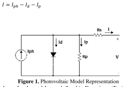
2. 1. Photovoltaic Model A photovoltaic panel (PV) module is represented as two nodes electrical circuit with the sunlight emulated as a current source, a diode connected in antiparallel, in a series and parallel resistances, as shown in Figure 1.
Then, the equation that defines the PV model dynamics in terms of an output current can be obtained via Kirchhoff’s current law, as shown in Equation (1).
𝐼 = 𝐼𝑝ℎ− 𝐼𝑑− 𝐼𝑝 (1)
Figure 1. Photovoltaic Model Representation
where, 𝐼𝑝ℎ,𝐼𝑑, and 𝐼𝑝 are defined in Equations (2), (3) and (4).
𝐼𝑝ℎ=𝐺𝐺
𝑟𝑒𝑓(𝐼𝑝ℎ,𝑟𝑒𝑓+ 𝜇𝑠𝑐∆𝑇) (2)
𝐼𝑑= 𝐼𝑜[exp (𝑉+𝐼∙𝑅𝛼 𝑠) − 1] (3)
𝐼𝑝=
𝑉+𝐼𝑅𝑠
𝑅𝑝
(4)
where, 𝐺 is the irradiance, 𝐺𝑟𝑒𝑓 is the irradiance at Standard Conditions, 𝑇𝑐 is the cells temperature, thus 𝑇 =
𝑇𝑐− 𝑇𝑐,𝑟𝑒𝑓 (𝑇𝑐,𝑟𝑒𝑓 = 298𝐾) and 𝜇𝑠𝑐 is the coefficient temperature of short circuit.
2. 2. Wind Turbine Model To model a wind turbine starts by defining the static and mechanical characteristics. The tip-speed ratio (TSR), denoted by 𝜆, is the radio between the linear speed as shown in Equation (5), calculated by the rotor radius and angular speed.
𝜆 =𝑟𝑟∙𝑤𝑟
𝑉𝑤 (5)
The TSR and the user-defined blade pitch angle, are used to calculate the rotor power coefficient, denoted by 𝐶𝑝 as shown in Equation (6) [11].
𝐶𝑝=
𝑃𝑟
𝑃𝑤 (6)
𝑃𝑤 is defined as the power of wind and 𝑃𝑟 is the power of rotor. Finally, the state equation is presented in the Equation (7), with the output in the current 𝑖𝑔. Where 𝐵𝑒𝑞 is the equivalent damping, 𝐾𝑒𝑞 is the equivalent hardness,
𝐽𝑟𝑒 is the reflected inertia, 𝐿𝐼 is the rotor electric inductance, 𝐿𝑔 the armature electric inductance and 𝑅𝑟𝑜𝑡 is the rotor electric resistance
[ 𝑤𝑟𝑒̇
𝜃𝑟𝑒̇
𝑖𝑔̇
] =
[
−𝐵𝐽𝑟𝑒𝑒𝑞 −
𝐾𝑒𝑞
𝐽𝑟𝑒 0
1 0 0
𝐿𝐼
𝐿𝑔 0 −
𝑅𝑟𝑜𝑡
𝐿𝑔]
[ 𝑤𝑟𝑒
𝜃𝑟𝑒
𝑖𝑔
] + [
1
𝐽𝑟𝑒
0 0
] 𝑇𝑟
𝑦 = [0 0 1] [ 𝑊𝑟𝑒
𝜃𝑟𝑒
𝑖𝑔
]
(7)
2. 3. Battery Model The Battery model can be expressed by the open circuit voltage (𝑉𝑜𝑐) or electromotive force (EMF) 𝐸𝑜, the battery voltage 𝑉𝑡, the internal resistance 𝑅𝑖, the discharge current 𝑖 and the State Of Charge (SOC) 𝑄 as shown in the Equations (8) and (9).
𝐸 = 𝐸0− 𝐾𝑄−∫ 𝑖 𝑑𝑡𝑄 + 𝐴𝑒 −𝐵 ∫ 𝑡 𝑑𝑡
(8)
𝑉𝑡= 𝐸 − 𝑅𝑖∙ 𝑖 (9)
constant and 𝐵 is the time constant inverse capacity. The battery voltage obtained is given by Equation (10).
𝐸𝑏𝑎𝑡𝑡= 𝐸𝑜− 𝐾 𝑄
𝑄−𝑖𝑡− 𝑅𝑖− 𝐾
𝑄
𝑄−𝑖 𝑖
∗+ 𝐴
𝑒
−𝐵𝑖𝑡
(10)
2. 4. Buck Converter Model The typology of Buck converter is shown in Figure , with a power switch 𝑆, inductor 𝐿 and capacitor 𝐶. The resistance 𝑅 represents the load on the battery circuit. This converter is attempted to emulate a diesel power source; which is commonly present in isolated power systems [12].
The dynamic process of the circuit can be described by the ordinary differential Equations (11) and (12). Buck response was controlled by a discrete time servo system.
𝐿𝑑𝑡𝑑𝑖= −𝑣 + 𝐸𝑢 (11)
𝐶𝑑𝑣
𝑑𝑡= 𝑖 − 𝑅𝑣 (12)
2. 5. Micro Grid System The micro-grid was designed to be modeled as shown in Error! Reference source not found..
Figure 2. Buck converter diagram
When the individual renewable source representation is obtained, it is integrated into the micro grid to get the final mathematical model, in this case is required the
application of linearization techniques that provides a lot of insight about its dynamics. From the above, a process of discrete-time system identification was helpful to get the linearization model, obtaining the Simulink representation shown in Error! Reference source not found.. In this tool is required define the operating point, in this case we use the model initial conditions as shown in Table 1.
The toolbox shows the state space, the zero-pole gain and the transfer function representation; it is implemented the transfer function in the Equation (13), to calculate a generalized predictive control.
𝐺(𝑧) =0.0002535 z3+1.31𝑒−5z2+5.381𝑒−5z−9.82𝑒−46
z4−z3+9.517𝑒−10z2−3.952𝑒−35z−8.246𝑒−67 (13)
3. CARIMA MODEL IN A GPC WITH MEASUREMENT DISTURBANCES MODEL
The common SISO transfer function model for GPC is the CARIMA model, because it considers the uncertainty that could have a non-zero steady state in its representation, so in Equation (15) is shown its mathematical expression [13]. Where 𝜍𝑘 = 0 means a random variable and 𝑇(𝑧) is treated as a design parameter. For convenience the CARIMA model can be expressed as shown Equation (16), where [𝑎(𝑧)∆] is a combination between 𝑎(𝑧) and Delta(∆), and ∆𝑢𝑘 use input increments with ∆= 1 − 𝑧−1 [14-16].
Figure 1. Micro Grid Representation
TABLE 1. Model Initial Conditions
Condition Value
Wind Turbine 0.0001
Battery model 498960
Buck Converter 1
Photovoltaic Panel 0
𝑎(𝑧)𝑦𝑘 = 𝑏(𝑧)𝑢𝑘+ 𝑑(𝑧)𝑣𝑘+ 𝑇(𝑧)
𝜍𝑘
𝛥 (15) where, 𝑑(𝑧)𝑣𝑘 is the representation of disturbances transfer function. For convenience, the CARIMA model can be expressed as shown in Equation (16), where
[𝑎(𝑧)𝛥 ] is a combination between 𝑎(𝑧) and delta (𝛥),
[𝑎(𝑧)𝛥]𝑦𝑘= 𝑏(𝑧)[𝛥𝑢𝑘] + 𝑑(𝑧)[𝛥𝑣𝑘] + 𝑇(𝑧)ς𝑘 (16)
Another way to represent the CARIMA model is through Equation (17). In SISO models 𝑏(𝑧) and 𝐴(𝑧) are given by the numerator and denominator of transfer function as shown in Equations (18) and (19). While 𝑑(𝑧) are given by the numerator of disturbance model as is shown in Equation (20).
𝐴(𝑧)𝑦𝑘= 𝑏(𝑧)[𝛥𝑢𝑘] + 𝑑(𝑧)[𝛥𝑣𝑘] + 𝑇(𝑧)𝜍𝑘 (17)
𝑏(𝑧) = 𝑏1𝑧−1+ ⋯ + 𝑏𝑚𝑧−𝑚 (18)
𝐴(𝑧) = 1 + 𝐴1𝑧−1+ ⋯ + 𝐴𝑛𝑧−𝑛 (19)
𝑑(𝑧) = 𝑑0+ 𝑑1𝑧−1+ ⋯ + 𝑑𝑝𝑧−𝑝 (20)
To have an appropriate notation it is considered the system in terms of matrix and vectors as shown in Equation (21).
𝑦𝑘+1= 𝐻 𝛥
→ 𝑢𝑘+ 𝑃 𝛥
← 𝑢𝑘−1+ 𝐸 𝛥
→ 𝑣𝑘+ 𝐺 𝛥
← 𝑣𝑘−1− 𝑄𝑦←𝑘
(21)
where, 𝐻 = 𝐶𝐴−1 𝐶𝑏 , 𝑃 = 𝐶𝐴−1 𝐻𝑏, = 𝐶𝐴−1 𝐶𝑑 , 𝐺 =
𝐶𝐴−1 𝐻𝑑y, 𝑄 = 𝐶𝐴−1 𝐻𝐴. The H, 𝑃, 𝐸, 𝐺 and 𝑄, matrix
dimension are determinates by the prediction and control horizons.
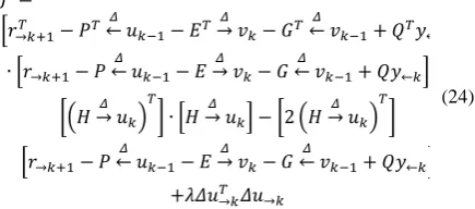
3. 1. Control Law To develop a GPC law algorithm the unbiased cost (𝐽) as shown in Equation (23) is defined. Where 𝑒𝑘+1= 𝑟𝑘+1– 𝑦𝑘+1, and 𝜆 is a constant value between 0 and 1, that determines the controller robustness.
𝐽 = 𝑒→𝑘+1𝑇 𝑒𝑘+1+ 𝜆𝛥𝑢→𝑘𝑇 𝛥𝑢→𝑘 (23)
It must consider the same unbiased cost showed in Equation (15). Consequently, we can perform a minimization to find the optimum 𝐽 value. So, considering the Equation (23), is necessary replace it to get a representation with the past and future values as shown in Equation (24) [17].
𝐽 = [𝑟→𝑘+1𝑇 − 𝑃𝑇
𝛥
← 𝑢𝑘−1− 𝐸𝑇 𝛥
→ 𝑣𝑘− 𝐺𝑇 𝛥
← 𝑣𝑘−1+ 𝑄𝑇𝑦←𝑘]
∙ [𝑟→𝑘+1− 𝑃 𝛥
← 𝑢𝑘−1− 𝐸 𝛥
→ 𝑣𝑘− 𝐺 𝛥
← 𝑣𝑘−1+ 𝑄𝑦←𝑘] +
[(𝐻→ 𝑢𝛥 𝑘) 𝑇
] ∙ [𝐻→ 𝑢𝛥 𝑘] − [2 (𝐻 𝛥
→ 𝑢𝑘) 𝑇
]
[𝑟→𝑘+1− 𝑃 𝛥
← 𝑢𝑘−1− 𝐸 𝛥
→ 𝑣𝑘− 𝐺 𝛥
← 𝑣𝑘−1+ 𝑄𝑦←𝑘]
+𝜆𝛥𝑢→𝑘𝑇 𝛥𝑢→𝑘
(24)
Considering the above equation, it can eliminate the past terms because they do not affect the values that should be minimized in the optimization rule.
In the optimization of the cost function 𝐽 exists an only minimum defined by a gradient equal zero, so the
optimum is given by Equation (25).
𝛥𝑢→𝑘=
(𝐻𝑇𝐻 + 𝜆𝐼)−1𝐻𝑇∙
[𝑟→𝑘+1− 𝑃 𝛥
← 𝑢𝑘−1− 𝐸 𝛥
→ 𝑣𝑘− 𝐺 𝛥
← 𝑣𝑘−1+ 𝑄𝑦←𝑘]
(25)
The control law equation is determined by a 𝑘 constant defines by the first row of matrix (𝐻𝑇𝐻 + 𝜆 𝐼 )−1 𝐻𝑇 multiply by 𝛥𝑢→𝑘 as shown in Equation (26) [18].
𝛥𝑢→𝑘=
𝑘(𝐻𝑇𝐻 + 𝜆𝐼)−1𝐻𝑇∙
[𝑟→𝑘+1− 𝑃 𝛥
← 𝑢𝑘−1− 𝐸 𝛥
→ 𝑣𝑘− 𝐺 𝛥
← 𝑣𝑘−1+ 𝑄𝑦←𝑘]
(26)
To design a block diagram simulation is required unpack each term of the 𝑢𝑘 equation in vectors as shown in Equation (27). Then the GPC control law is summarized as is shown in Equation (28).
𝑃𝑟= 𝑘(𝐻𝑇𝐻 + 𝜆𝐼)−1𝐻𝑇
𝐷𝑘= 𝑃𝑟𝑃
𝑁𝑘= −𝑃𝑟𝑄
𝑅𝑘= 𝑃𝑟𝐸
𝑆𝑘= 𝑃𝑟𝐺
(27)
𝛥𝑢𝑘= 𝑃𝑟𝑟→𝑘+1− 𝐷𝑘𝛥𝑢𝑘− 𝑅𝑘 𝛥
→ 𝑣𝑘+1− 𝑠𝑘 𝛥
← 𝑣𝑘− 𝑁𝑘𝑦←𝑘
(28)
The final representation 𝑢𝑘 is shown in Equation (29).
𝑢𝑘= [(1 − 𝐷𝑘)𝛥]−1(𝑃𝑟𝑟→𝑘+1− 𝑅𝑘 𝛥
→ 𝑣𝑘+1− 𝑠𝑘 𝛥
← 𝑣𝑘− 𝑁𝑘𝑦←𝑘)
(29)
4. RESULTS AND DISCUSSION.
Then, the GPC behavior is simulated as structure shown in the Error! Reference source not found..
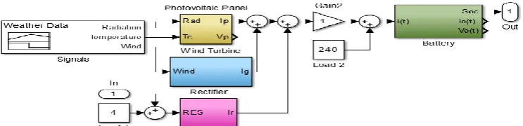
Considering the above, Figure 2 shows the block simulation in Simulink/MATLAB. Which proposes a control block followed by a Switch System block that allows charge the battery in specific cases, a Rectifier block that give the current to charge the batteries and a Measurement Disturbances block.
To develop the control system, a control horizon of 320, and prediction horizon of 720, with a lambda of 1. Then, it is obtained as result a charge battery behavior in Error! Reference source not found. with disturbances, with a signal control in Error! Reference source not found. and rectifier response in Error! Reference source not found..
Figure 2. Micro Grid control diagram
Figure 6. Behavior of Battery Charge with GPC 80% SOC
Figure 7. Control Signal with Disturbances
Figure 3. Rectifier Signal Response with Disturbances
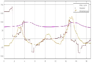
In this case, in order to decrease the controller’s response time with the intention of avoid big numerical data, which would diminish the embedded controller on the STM32 performance, it was added a couple of zeros and delays on the equation. As result, it shows signals peaks of 300 and less on the control signal, what generates that the time in which the rectifier is saturated, it is not too long, until this reaches the desired reference. The rectifier is saturated at 200 A due its electrical characteristics, which only allow 200A as maximal current of charge.
Once the controller was designed, it was tested under
different types of desired references. The response simulating ideal SOC and the desired behavior of battery charge is shown in Figure 9. It is attempted a cycle of charge and discharge intended to emulate an entire micro grid system duty cycle. Figure 10 shows the rectifier behavior with disturbances and working under a micro grid system duty cycle.
The micro grid system duty cycle was designed in order to maximize the batteries cycle life, that in accordance with their data sheet, it must not exceed 30% of depth of discharge. This duty cycle variates from 70 to 95% the SOC and emulates 2 days of continue work at the micro grid facilities located inside the Nueva Granada Military University Campus.
It is worthy to note that the rectifier signal represents how the diesel plant would act in an isolated power system, as a hybrid power system.
After the corresponding tests to the designed GPC, it was embedded inside a STM32F446 development board, this kind of boards provide an affordable and flexible way to fast prototyping.
Figure 9. Response simulating ideal %SOC according to the
desire behavior of Battery Charge
Figure 10. Rectifier response according micro-grid system
This development board offers a perfect combination of performance, power consumption and features that match with the requirements to integrate the GPC designed and adapt it to our micro-grid DC.
Once embed the controller on the STM32, it was embedded the plant equivalent equation on an
ARDUINO MEGA. Taking advantage of the
characteristics of compatibility between this two development boards. First, it was tested that the GPC was able to be embedded on a relatively small microcontroller despite of the robustness of this kind of controllers regarding to process memory consumption. Once the GPC was embedded on the Development Board, it was measured the time taken for each process from the GPC Table 2.
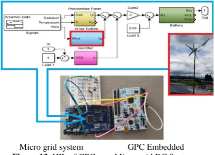
Figures 11 and 12 show the block diagram corresponding to the micro-grid DC system embedded on the Arduino Mega and the GPC embedded on the STM32, respectively. The system in Figure 13 shows how the connection between the two boards was done.
The system response was tested and monitored from Matlab through Simulink’s external simulation mode and the data were captured by RS232 serial communication. Based on the time elapsed per cycle, Table 2; several sample times were tried in pursuit of identify the best for this application. As result was found that the best sample time is up to 10 seconds and lower than 10 minutes; smaller time would increase the memory consumption on the board and would be useless because the behavior of the micro-grid DC system. The response time of charge and disturbance are not fast, they change in a slow and proportional way under normal conditions.
TABLE 2.Process time for the GPC.
Process Time (s)
Calculating GPC model. 2.091487
Dk Filter 0.265625
Nk Filter 0.156250
Pr Filter 0.07812500
Total time elapsed 1 cycle 2.591597
Figure 11. Micro-grid DC System Embedded on Arduino
Mega
Figure 12. GPC Embedded on STM32F446
Micro grid system GPC Embedded
Figure 13. HIL of GPC on a Micro-grid DC System
5. CONLUSIONS
This paper has shown that GPC implemented on a micro grid system is possible and enhance the performance of this kind of systems; taking advantage of the properties of these predictive controllers, it prevents non-desire inputs and outputs through defining constraints previously, drives some output variables to the optimal set points, while maintaining other outputs within specified ranges, between others.
As it is shown in this article, predictive control strategies would decrease the use of fossil fuels, because this technique would allow to determine when the battery power bank won’t have the enough amount of stored energy to maintain the power service. Therefore, diesel plant would start working in a low consumption mode (increasing the diesel plant efficiency) before power system runs out, providing in a long term the predicted amount of energy necessary to satisfy the demand of the load.
This controller has shown an optimal working under disturbances presence and accomplished its aim according the expectations. It was possible to embedded
this controller in the micro grid using
Simulink/MATLAB and simulate its performance in the micro grid model, it’s expecting to apply these methods of prediction improving the efficiency of this micro grids and minimizing the use of fossil fuels to generate energy. Further works are leading to implement this controller on multivariable systems, such as two micro-grid DC or more, looking for optimize the existing system creating a small smart grid.
6. ACKNOWLEDGEMENT
7. REFERENCES
1. Mauledoux, M., Mejía-Ruda, E. and Caldas, O.I., "Multiobjective evolutionary algorithms moea to solve task allocation problemsin multiagent systems for dc microgrid", Applied Mechanics & Materials, Vol. 700, No. 4, (2014), 24-27.
2. ME, R.S.R.B., ME, S.D. and ME, S.J., "A closed loop control of quadratic boost converter using pid controller", International Journal of Engineering-Transactions B: Applications, Vol. 27, No. 11, (2014), 1653-1662.
3. Devabhaktuni, V., Alam, M., Depuru, S.S.S.R., Green II, R.C., Nims, D. and Near, C., "Solar energy: Trends and enabling technologies", Renewable and Sustainable Energy Reviews, Vol. 19, No., (2013), 555-564.
4. Commission, F.E.R., "Assessment of demand response and advanced metering", (2008).
5. Mork, B. and Weaver, W., "Smart grids and micro-grids: What are they really", in Minnesota Power Systems Conference. (2009), 3-5.
6. Gholizade-Narm, H., "A novel control strategy for a single-phase grid-connected power injection system", International Journal of Engineering-Transactions C: Aspects, Vol. 27, No. 12, (2014), 1841-1849.
7. Ara, A.L., Tolabi, H.B. and Hosseini, R., "Dynamic modeling and controller design of distribution static compensator in a microgrid based on combination of fuzzy set and galaxy-based search algorithm", International Journal of Engineering-Transactions A: Basics, Vol. 29, No. 10, (2016), 1392-1400.
8. Clarke, D.W., Mohtadi, C. and Tuffs, P., "Generalized predictive control—part i. The basic algorithm", Automatica, Vol. 23, No. 2, (1987), 137-148.
9. Chidrawar, S. and Patre, B., "Generalized predictive control and neural generalized predictive control", Leonardo Journal of Sciences, Vol. 7, No. 13, (2008), 133-152.
10. Holkar, K. and Waghmare, L., "An overview of model predictive control", International Journal of Control and Automation, Vol. 3, No. 4, (2010), 47-63.
11. Tang, C.Y., Guo, Y. and Jiang, J.N., "Nonlinear dual-mode control of variable-speed wind turbines with doubly fed induction generators", IEEE Transactions on Control Systems Technology, Vol. 19, No. 4, (2011), 744-756.
12. Katiraei, F. and Abbey, C., "Diesel plant sizing and performance analysis of a remote wind-diesel microgrid", in Power Engineering Society General Meeting, 2007. IEEE. (2007), 1-8. 13. Ordys, A.W., "Predictive control for industrial applications",
Annual Reviews in Control, Vol. 25, (2001), 13-24.
14. Rodríguez, P. and Dumur, D., "Generalized predictive control robustification under frequency and time-domain constraints",
IEEE Transactions on Control Systems Technology, Vol. 13, No. 4, (2005), 577-587.
15. Guo, W., Wang, W. and Qiu, X., "An improved generalized predictive control algorithm based on pid", in Intelligent Computation Technology and Automation (ICICTA), 2008 International Conference on, IEEE. Vol. 1, (2008), 299-303.
16. Zhou, L. and Qu, D., "Study of generalized predictive control scheme and algorithm based on artificial neural network", in Information Acquisition, 2006 IEEE International Conference on, IEEE. (2006), 1208-1212.
17. Hou, G., Bai, X. and Huang, R., "Application of improved generalized predictive control to coordinated control system in supercritical unit", in Industrial Electronics and Applications (ICIEA), 2014 IEEE 9th Conference on, IEEE. (2014), 1591-1595.
18. Fioriti, D., Giglioli, R., Poli, D., Lutzemberger, G., Vanni, A. and Salza, P., "Optimal sizing of a hybrid mini-grid considering the fuel procurement and a rolling horizon system operation", in Environment and Electrical Engineering and 2017 IEEE Industrial and Commercial Power Systems Europe (EEEIC/I&CPS Europe), 2017 IEEE International Conference on, IEEE., (2017), 1-6.
Hardware in Loop of a Generalized Predictive Controller for a Micro Grid DC System
of Renewable Energy Sources
O. Rivera, M. Mauledoux, A. Valencia, R. Jimenez, O. Avilés
Mechatronics Engineering Department, Universidad Militar Nueva Granada, Bogota, Colombia
P A P E R I N F O
Paper history:
Received 16 February 2018 Received in revised 27 April 2018 Accepted 02 July 2018
Keywords:
Generalized Predictive Control Hardware in the Loop Micro-grid STM32
هديكچ
( هقلح یزاس هیبش رد رازفا تخس کی ،هلاقم نیا رد
HIL
یارجا زا لبق مدق نیلوا ناونع هب همانرب نیا .تسا هدش هئارا )
شیپ لرتنک کی یعقاو ( یمومع ینیب
GPC
رد یماظن هاگشناد سیدرپ رد عقاو هکبش ورکیم متسیس کی یور رب )
Cajica
،
.تسا ایبملک
GPC
( ژراش تلاح رد یرتاب ژراش هک دور یم راظتنا ،تسا هدش یحارط
SOC
زا شیب )
70 ٪
زا رتمک و
90 ٪
ک یم نیمضت نآ ینف تاصخشم هب هجوت اب یرتاب رد ار درکلمع نیرتهب هک ،دشاب متیروگلا .دن
GPC
رلرتنکورکیم کی یور رب
STM32
رلرتنکورکیم کی یور رب هکبش ورکیم لدم و تفرگ رارق
ARDUINO MEGA
.دش هیبعت