International Journal of Finance and Managerial Accounting, Vol.2, No.6, Summer 2017
1
With Cooperation of Islamic Azad University – UAE Branch
Simulation of Long-term Returns with
Stochastic Correlations
Giorgio Consigli
Department of Mathematics, Statistics and Computer Science, University of Bergamo, Via dei Caniana, 24127 Bergamo, Italy (Corresponding author)
Mohammad Mehdi Hosseinzadeh
Department of Mathematics, Statistics and Computer Science, University of Bergamo, Via dei Caniana, 24127 Bergamo, Italy
ABSTRACT
This paper focuses on a nonlinear stochastic model for financial simulation and forecasting based on assumptions of multivariate stochastic correlation, with an application to the European market. We present in particular the key elements of a structured hierarchical econometric model that can be used to forecast financial and commodity markets relying on statistical and simulation methods. The investment universe includes money-market, fixed-income, inflation-linked bonds as well as equity and commodity indices. For each such investment opportunity a dedicated statistical model has been developed to generate future return paths describing the uncertainty the investment manager is facing over time.
Keywords:
1. Introduction
A crucial issue for consistent financial management is an accurate econometric modeling of market conditions, sometimes over long-term horizons. The dynamic behavior of market values is dependent on random factors such as interest and inflation rates, the economic cycle and correlation among assets.
The recent sovereign crisis in Europe (2009-2011) has deeply affected previous financial markets conditions leading to a phase of unprecedented monetary easing and low interest rates, which unlike in the past, were not effective in recovering market stability and economic growth. In particular the European market suffered from increasing default risk of selected sovereign borrowers and increasing correlation and systemic risks in the Euro zone. In this situation, investments, which had long-term horizon plans, were faced with a downside potential of the financial markets in many countries. During such periods of market fluctuation, the adoption of a dynamic asset return model for securities exposed to market risk may play a crucial role. By focusing on market prices, we propose in this work a simulation approach to incorporate stochastic correlations in a two-layer multivariate statistical model.
We consider a simulation approach based on a hierarchical econometric model with EU GDP and inflation rate considered as the basic driving forces from which further economic factors, such as short and long-term interest rate and asset returns, are derived. The financial risk factors and asset returns are modeled with parameters and correlations fitted to quarterly data.
In this article, we develop and test a long-term asset returns simulation method in a two-level fashion with a dynamic stochastic correlation model and relying on a realistic asset universe, with interest-rate sensitive assets, such as government and inflation linked bonds, money market fund, equity, commodities. The stochastic model presented in section 1 extends [6], where a stochastic mean and constant correlation model was employed in an individual asset-liability management problem. Several statistical models are currently in use to simulate asset price and returns for the solution of decision problems under uncertainty. We refer to [21] which was among the first to introduce a cascade structure for asset price return simulation, later
adopted by [11] with CASM (Cascade Asset Simulation Model) and [1]. A practical approach to include an assumption of stochastic correlations in a two-layer asset simulation and test its effectiveness are the main objectives of this article.
Stochastic correlation was introduced as dynamic conditional correlation (DCC) model by [16] with analyzing the performance of the model for large covariance matrices. DCC method has been used in the econometric and financial problems. We cite some of the most relevant contributions [12, 3, 13, 22, 19, 23, 15, 9].
The article is structured in 4 sections. In section 2 we introduce stochastic correlation and long-term asset returns simulation in a two-layer structure. In section 3 we apply the model and show the returns simulation results and in Section 4 we conclude
2. Asset Returns Simulation
With simulation techniques, many possible future situations of a financial portfolio can be evaluated. In financial planning the unfolding uncertain future is represented by a large number of future paths from the simulation process which uses Monte Carlo simulation technique [17] to investigate the evolution of asset returns over planning horizon. This is an advantage of the simulation that we can use a relatively large number of scenarios for the future circumstances.
For any financial planning problem, we need to know about behavior of our assets over time horizon. Since market conditions are changing over time and exposed to stochastic factors, we introduce an asset returns model in discrete-time with a modeling framework based on Two-Layers Asset Simulation Model (TLASM) with stochastic correlation among assets. The multivariate statistical model can reflect market dynamics during instability periods.
2.1. Stochastic correlations
constraints requires a forecast of the covariance matrix of the returns. Similarly, the calculation of the standard deviation of today’s portfolio requires a covariance matrix of all the assets in the portfolio. Simple methods such as rolling historical correlations and exponential smoothing are widely used. More complex methods such as varieties of multivariate GARCH or Stochastic Volatility have been extensively investigated in the econometric literature [20, 16, 2, 13].
We consider a dynamic conditional correlation (DCC) model [12] and then present an approach for asset returns simulation consistent with such assumption. Let
, i t
r be the return of asset
i
I
at timetT. We indicate with
r
t the return vector withcomponents , i t
r . Given r0 and
( , , )
F P
as ageneric random source of risk, for
t=1,2,...,T
, we define the stochastic differential equations for return process as:( , ) ( , ) ( )
t t dt
r r
t dt t
dte
(1)
where
( , )
t
dt
is an instantaneous drift. We assume in section 1.2 dedicated models for different asset indexes. ( , )t
is a random covariance matrixthat admits decomposition
t D C Dt t t
and
(0,1)
e N .
t
Dis a diagonal matrix with elements
, i t
with i1, 2,...,I, includes the Ireturns’ conditional
standard deviations which can be defined by any type of a univariate GARCH process, while Ct: { cij t,}
includes the time-varying correlation coefficients
between asset
i
and assetj
at timet
.The DCC is a natural extension of the GARCH models. In the DCC model [12] the relationship between conditional correlations and conditional
variance was obtained expressing the returns,
r
i t, as, , ,
i t i t i t
r
where, ~ (0,1)
i t N
.
(2)
We assume a Threshold Autoregressive
Conditional Heteroskedasticity (TARCH) process of
the first order for
i t2, . [18] and [24] introducedindependently the TARCH models which allows for asymmetric shocks to volatility. According to [14], TARCH volatility process is a way of parametrizing the sign of the innovation that may influence the volatility in addition to its magnitude.
In DCC model [12], the conditional correlation matrix is modeled as:
0.5 0.5
t t t t
C Q Q Q
(3)
Where
Q
t
{
q
ij t,}
is the conditional covariancematrix and t
Q is the diagonal matrix of the i th
diagonal element of the
Q
t. Dynamics ofQ
t can beconsider with following the DCC model [12] assumption as:
1 1 1
(1 )
t t t t
Q
Q
Q(4)
where Qis the unconditional correlation matrix of
. α and β are constant parameters such that , 0and
1to ensure positive definiteness andstationarity, respectively. Accordingly, the variance-covariance process dynamics can be expressed as
0.5 0.5
( )
t D Qt t Q Qt t Dt
(5)
1.1.
2.2. Two-Layers Asset Simulation
Model
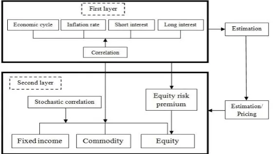
According to the figure 1, in this model we consider two layers structure, at the first layer we derive the relative risk factors then in the second layer compute the equity risk premium and returns of each asset class.
Structure of the risk model includes all market variables adopted to derive the benchmarks’ evolution: money market benchmark, bond indexes, equity and commodity benchmarks [21, 4, 8, 1, 11, 10, 6].
Table 1 includes Euro area market benchmark indexes and the associated risk factors of each investment opportunities in this study. We consider inflation rate, GDP output gap and 12-month Euribor together with 10 years Euro interest rate as short and long-term interest rate in our risk factor modeling. Inflation and interest rates are two critically important
risk-factors for any financial investment. In particular assets can suffer of inflation shocks because an inflation increase normally triggers an interest rate upshift thus negatively hitting the fixed income nominal assets. We refer here to the risk process as the random process of the financial factors embodying the risk sources of the problem [8, 5, 6].
We translate a set of continuous stochastic dynamics into a discrete event structure relies on a scenario tree labeling
Figure 1: Structure of two layers asset simulation model
scheme [7]. Nodes along the tree, for
t
T
, are denoted by nNt. For t = 0 the root node(associated with the partition
0 { , }
N ,
corresponding to the entire probability space) is labeled n = 1.
For t > 0 every
n
N
thas a unique ancestorn− and, for t < T, a non-empty set of children nodes n+.
We denote with
t
n the time associated with node n.The set of all predecessors of node
n
: n n, ,..., 0isdenoted by
n
P. From the statistical modeling
viewpoint, first layer risk factors
, j n
plus equity risk premium
n
and then second layer asset price return
,
i n
r
are computed with multivariate Gaussian returnmodel with autoregression and exogenous variables. Stochastic difference equation for risk factors j n, for j
= 1,2,3,4 and equity risk premium
n for allt
nN
are considered as follow:
, , ,
r
j n j n j j r n
r j
t c e
(6)
where vector
j n, gives the following stochastic driftof the risk factors at nod
n
:1 1 1
0 1 1, 2 1,
2 2 2 2 2
0 1 2, 2 1, 3 1, 4 1,
,
3 3 3
0 1 2, 2 1,
4 4 4 4
0 1 4, 2 1, 3 2,
1 2 3 4 n n n
n n n
j n
n n
n n n
j j j j (7)
0 1 4, 2 2,
n n n ten
Table 1: Market benchmarks and relative risk factors
Investment Class Benchmark Risk factors
Money market Euribor 12 month Inflation rate, economic cycle, 12-month short rate
European Gov. bond JPM Global Emu Euro stock, interest rate, economic cycle
- JPM Global ex-EMU Euro stock, inflation rate
Inf. Link. bond Barclays Infl. Linked Euro stock, interest rate, inflation rate
Equity MSCI Europe Index Stock risk premium, interest rate
Commodity Dow Jones Comm. Euro stock, economic cycle, euro bond market
The risk factors
j for j = 1,2,3,4 defined as:
1is the GDP output gap,
2 is the inflation rate,
3isthe short interest rate and
4 is the long interest rate.In the model,
t
defines the time increment between nodes n− and n. Risk factors correlation is introduceddirectly on the realizations
e
nr of four standard normalvariables through the Cholesky elements
c
j r, of thecorrelation matrix with normal distribution
N
(0,1)
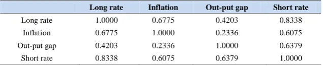
and illustrated in Table 3.
The set of estimated coefficients and risk factors provides an input to the generate the asset returns scenarios and will determine the returns’ evolution over the long-term decision horizon. The asset
returns simulation of each benchmark
r
i n, in eachnode
n
N
t for scenario generation can now bedetermined as following formulas for the different benchmark indexes:
Europe bonds:
, 0 , , , , ,
i r
i n i n i n i n i r n n
r
r
r
t
c
e
2,3, 4
i
(9)where vector
i n, defined stochastic drift at node n asfollows:
2 2 2 2
1 2 5, 3 1, 4 4,
3 3 3
, 1 2 5, 3 2,
4 4 4 4
1 2 2, 3 5, 4 4,
2 3
4
n n n
i n n n
n n n
r i
r i
r i
(10)
For the European bonds
r
i (i = 2,3,4), we considerr
2as JPM Global Government Bond EMU index,
r
3 forthe JPM Global Government Bond ExEMU index and
4
for the Barclays Euro Inflation Linked bond index.In the statistical models, coefficients show the dependence of the government bonds return with the stock risk premium.
Equity:
• MSCI Europe equity
5,n (1,n n) 5,n i r n, , n r
r r t
c e(11)
The equity return is modeled relying on the performance of the equity risk premium (see equation 8) and short-term interest rate in Euro zone. The risk premium is depended on the long-term interest rate, inflation rate and economic cycle.
Indirect real asset:
• Commodities
6 6 6 6
6,n 1 2 5,n 3 4,n 4 1,n
r r r
6
5 2, 6, 6, ,
r
n n r n n
r
t c e
The commodity return is evaluated by a stable relationship with the GDP output gap, inflation rate, equity market and Euro inflation linked bond yields.
2.3.
Statistical
Assumptions
and
Estimation
The economic and financial risk factors are modeled with parameters and correlations fitted to quarterly data in a two level TLASM fashion.
We use delegate total return indices for the asset classes. A total return index includes the reinvestment of dividends in the case of stock markets and the gains or losses of the price variation in the case of bond markets, respectively. All of the mentioned data sets have been collected at a quarterly frequency through the Data-Stream source. Furthermore, for all data sets, the time-specified of past observed market data starts from January 1999 and ends in December 2015. The statistical coefficients are estimated through the method of ordinary least squares (OLS) (see table 2 and 3). Risk factors correlation matrix estimated and reported in Table 4.
3. Simulation Results
The numerical results have been computed through a MATLAB R2014a for simulation and Excel as the input and output data collection. The simulation has
been generated with 2048 number of paths at the horizon.
We consider a discrete simulation model over the 10-year planning horizon from Q1 2009 include investment universe based on the table 1.
To show the complex nature of the output from TLASM with stochastic correlation, forward scenario tree generation of the corresponding asset class returns have been performed by back-tested analysis with quarterly data from Q1 2009 to Q4 2016.
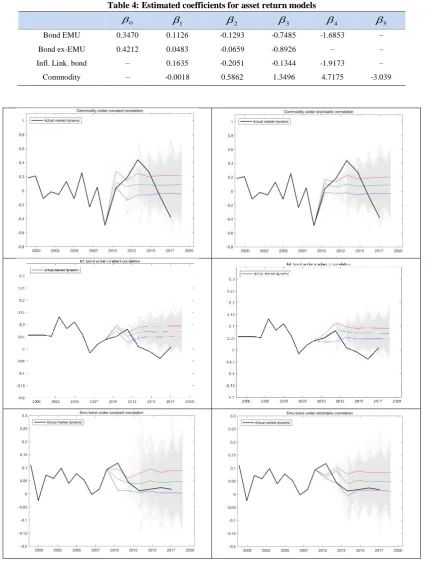
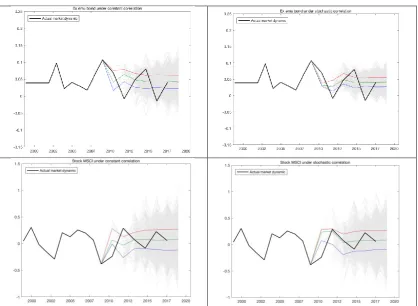
We show in figure 2 a set of output trees generated for representative asset index classes based on the introduced simulation model with stochastic -right side- versus constant correlation -left side- models. The simulation is generated across time with respect to observed market dynamic at each stage up to Q4 2015. The different techniques for simulation are ex-post analyzed on actual market dynamic with same estimated coefficients and assumption.
We consider the periods of 2009 until 2016 which crisis, post crisis and recent market situation took place. In almost all cases the asset returns simulation with stochastic correlation includes actual market value over the simulation period seen to that date which includes also recent market instability.
Table 2: Risk factors estimated coefficients and volatilities
0
1
2
3
4 Vol. (%)Out-put gap 0.0002 1.8095 -0.8950 – – 1.14
Inflation 0.0123 0.4317 -0.6236 1.4184 -0.8012 0.92
Short rate 0.0391 -0.2483 0.5889 – – 1.53
Long rate 0.0191 0.7749 0.0873 -0.4572 – 1.41
Risk premium 1.0564 -13.2855 -21.2597 – – 20.07
Table 3: Risk factors correlation matrix
Long rate Inflation Out-put gap Short rate
Long rate 1.0000 0.6775 0.4203 0.8338
Inflation 0.6775 1.0000 0.2336 0.6075
Out-put gap 0.4203 0.2336 1.0000 0.6379
Table 4: Estimated coefficients for asset return models
0
1
2
3
4
5Bond EMU 0.3470 0.1126 -0.1293 -0.7485 -1.6853 –
Bond ex-EMU 0.4212 0.0483 -0.0659 -0.8926 – –
Infl. Link. bond – 0.1635 -0.2051 -0.1344 -1.9173 –
Figure 2: Asset returns scenario simulation of investment universe under constant correlation -left side and stochastic correlation -right side- (green trajectory is the mean scenario, purple and red trajectories 25% and 75% quantile of the distribution, respectively) with components related to the modelling of time series
for commodities and financial markets.
4. Conclusion
We have presented a simulation approach for long-term returns that, building on concepts from existing methods, integrates a set of economic and statistical requirements in a computationally efficient scheme. The method has been developed based on the idea of two-layer simulation model using stochastic correlations for financial problems, which may lead to a sufficient representation of the randomness underlying the decision-making process. This technique has been tested on actual market dynamic and we report evidence of its effectiveness compare to the method with constant correlation. Since there is correlation clustering changing dynamically during and after the crisis therefore introducing stochastic correlation among assets into simulation method is needed in order to approximate return distribution. We
presented effectiveness result of returns distribution under stochastic correlation versus constant correlation. The numerical evidence supports this method to yield a good approximation of a distribution with a long-term planning horizon. The methodology can be adopted for the formulation of optimization problems in financial and commodities markets.
References
3) Cappiello, L., Engle, R. F., & Sheppard, K. (2006). Asymmetric dynamics in the correlations of global equity and bond returns. Journal of Financial econometrics, 4(4), 537-572.
4) Consigli, G., & Dempster, M. A. H. (1998). Dynamic stochastic programming for asset-liability management. Annals of Operations Research, 81, 131-162.
5) Consigli, G., di Tria, M., Gaffo, M., Iaquinta, G., Moriggia, V., & Uristani, A. (2011). Dynamic portfolio management for property and casualty insurance. In Stochastic Optimization Methods in Finance and Energy (pp. 99-124). Springer New York.
6) Consigli, G., Iaquinta, G., Moriggia, V., di Tria, M., & Musitelli, D. (2012). Retirement planning in individual asset-liability management. IMA Journal of Management Mathematics, 23(4), 365-396.
7) Consigli, G., Iaquinta, G., & Moriggia, V. (2012). Path-dependent scenario trees for multistage stochastic programmes in finance. Quantitative Finance, 12(8), 1265-1281.
8) Cox, J. C., Ingersoll Jr, J. E., & Ross, S. A. (1985). A theory of the term structure of interest rates. Econometrica: Journal of the Econometric Society, 385-407.
9) D’Ecclesia, R. L. (2017). Time Varying Correlation: a Key Indicator in Finance. In Consigli G., Stefani S. & Zambruno G., editors, Recent advances in Commodity and Financial Modeling: Quantitative methods in Banking, Finance, Insurance, Energy and Commodity markets. International Series in Operations Research and Management Science. Springer, forthcoming.
10) Dempster, M. A. H., Germano, M., Medova, E. A., Murphy, J. K., Ryan, D., & Sandrini, F. (2009). Risk profiling defined benefit pension schemes. To appear in: Journal of Portfolio Management. 11) Dempster, M. A., Germano, M., Medova, E. A., &
Villaverde, M. (2003). Global asset liability management. British Actuarial Journal, 9(01), 137-195.
12) Engle, R. (2002). Dynamic conditional correlation: A simple class of multivariate generalized autoregressive conditional heteroskedasticity models. Journal of Business & Economic Statistics, 20(3), 339-350.
13) Engle, R. (2009). Anticipating correlations: a new paradigm for risk management. Princeton University Press.
14) Engle, R. F., & Patton, A. J. (2001). What good is a volatility model. Quantitative finance, 1(2), 237-245.
15) Engle, R., & Figlewski, S. (2015). Modeling the dynamics of correlations among implied volatilities. Review of Finance, 19(3), 991-1018. 16) Engle, R. F., & Sheppard, K. (2001). Theoretical
and empirical properties of dynamic conditional correlation multivariate GARCH (No. w8554). National Bureau of Economic Research.
17) Glasserman, P. (2003). Monte Carlo methods in financial engineering (Vol. 53). Springer Science & Business Media.
18) Glosten, L. R., Jagannathan, R., & Runkle, D. E. (1993). On the relation between the expected value and the volatility of the nominal excess return on stocks. The journal of finance, 48(5), 1779-1801. 19) Hafner, C. M., & Franses, P. H. (2009). A
generalized dynamic conditional correlation model: simulation and application to many assets. Econometric Reviews, 28(6), 612-631.
20) Kim, S., Shephard, N., Chib, S. (1998). Stochastic volatility: likelihood inference and comparison with ARCH models. The review of economic studies, 65(3), 361-393.
21) Mulvey, J. M. (1996). Generating scenarios for the Towers Perrin investment system. Interfaces, 26(2), 115.
22) Pesaran, B., & Pesaran, M. H. (2007). Modelling volatilities and conditional correlations in futures markets with a multivariate t distribution.
23) Silvennoinen, A., & Thorp, S. (2013). Financialization, crisis and commodity correlation dynamics. Journal of International Financial Markets, Institutions and Money, 24, 42-65. 24) Zakoian, J. M. (1994). Threshold heteroskedastic