Summary
Maastricht University is offering a MBA program for people that have a bachelor degree and at least 5 years of working experience. Within the MBA program, students work in groups of 5 during a two year cycle. This thesis is about the formation of the student groups. The MBA program contains 60 students. Every year, two intake moments take place that usually allow 15 new students to enter. All 60 students follow the same course at the same time, implying that the order in which a student follows the courses depends only on the moment at which he/she starts the program. Every two periods, The university creates new student groups according to a set of hard and soft constraints, such that well-diversified groups are formed. Therefore, the student-with-student history, gender, nationality, and level of expertise of each student is taken into account. Hence a mapping from a set of students to groups is created that takes into account the corresponding constraints. The university chooses a group leader for each group.
Two general solution methods are applied to the MBA sectioning prob-lem. The first method uses the simplex algorithm to solve the probprob-lem. Therefore an integer linear program formulation of the problem was needed, and used as an input for an efficient ILP solver. The second approach starts with an initial feasible solution and improves upon this feasible solution us-ing different improvement algorithms. The quality of each feasible solution depends on the calculated objective function value that measures the level of satisfaction of the different constraints. Different initial solution and im-provement algorithms are discussed that help to obtain a feasible solution with an objective function value that is as low as possible. The imple-mented improvement algorithms are the Descent Improvement algorithm, Tabu Search, Simulated Annealing, and the Bipartite Weighted Matching Improvement algorithm. The first three algorithms make individual students swap between existing group formations. The Bipartite Weighted Matching Improvement algorithm iteratively selects a student from each group, and finds local optimal solutions for a bipartite matching problem in order to improve the overall objective value of the whole problem.
4.1. INTRODUCTION 101
4.1
Introduction
Many schools and universities in today’s society face the task of allocating students, children, or teachers to different groups. For example, starting with primary schools, groups are created for all kinds of activities. Each of these groups may be created according to different preferences. One prefer-ence could be not to have too many boys in one group. Moreover, teachers may be grouped together and have to be allocated to classes in order to make feasible and desired teacher-class combinations. For example in pri-mary schools, there exists the challenge of assigning parttime and full-time working teachers to different grades such that teachers are not continuously teaching the same children, and that furthermore working hour preferences are taken into account. Also in universities, allocation of students to groups, also known as sectioning of groups, takes place. A widely studied topic in the literature is the problem of ultimately sectioning university students with the same course into groups that will have the course at the same moment, to prevent and decrease overlap of student timetables. The following prob-lem, which is most closely related to the latter problem from above, will be discussed in depth and is the main focus in this thesis. In this bachelor thesis, the student sectioning problem of the MBA program at the School of Business and Economics faculty of Maastricht University (SBE) is analyzed and solved by different methods. These methods will be compared to find the most efficient and effective methods that lead to high quality solutions. Similar to the other problems above, here groups of students have to be formed. Aspects such as nationality, gender division, level of expertise, and team member histories of students are taken into account to create groups that are in accordance with the preferences.
4.2
Problem Description & Modeling
4.2.1
Problem Description
This thesis discusses the MBA student sectioning problem at the SBE. To obtain a Master of Business Administration (MBA), one has to follow a program of at least two years. To be classified as a candidate for the MBA program, you need at least five years of working experience. The problem of the SBE is to allocate the students of the MBA program to groups, such that the soft and hard constraints are satisfied. Stated differently, a mapping from a set of students to groups will be created that takes into account the corresponding hard and soft constraints. After a short introduction on the aspects of the MBA program, we continue with the general problem description and its constraints.
Each year, during each module of the program, a single course is given to all students at a time. For each of these modules, group divisions are established. Each module may consist of more than one course which are given sequentially, but the courses in one module have the same teams. On top of the normal modules, the MBA students also need to follow residen-tial weeks during the program. The MBA program consists of six modules and six residential weeks. The order in which a student follows the courses depends only on the moment at which he/she started the program. Addi-tionally, every student will do all modules. To make things clear, Figure 4.1 shows the complete MBA program with its corresponding modules, periods, intake moments and courses.
4.2. PROBLEM DESCRIPTION & MODELING 103
tried to keep these conflicts to a minimum. (ii) Students that are just
starting the MBA program are preferably allocated to groups that contain
students that have a higher level of expertise within the program. (iii)It
is desired to cluster students together in such a way that a good mixture
of nationalities/languages is created. (iv) Female students are preferably
equally divided among the groups, such that no groups of only women exist. Hence the definition of specific problem is as follows:
Definition 1. MBA student sectioning is the assignment of students to groups, such that:
1. Student-with-student histories are taken into account to create diver-sified groups.
2. A good mixture of nationalities is created.
3. There is a fair mixture of gender among the groups.
4. No group contains only students that are just starting the MBA pro-gram.
Figure 4.1: MBA cycle
residential weeks, students have to work in groups of six people. When the amount of students that are participating is not a multiple of six, some of the groups are allowed to be of size five. The sectioning of students for the residential weeks further faces the identical constraints that are applicable for the regular module student-sectioning problem. The sectioning of students for modules and residential weeks happens in an alternating matter, which is also confirmed by Figure 4.1 on the previous page. It is preferred to take the student history for both the residential weeks and the regular modules into account at the same time, but if scheduling problems occur, we separate the student histories for both the module and residential problem. For example, for a module group sectioning, in this case only the history of previous modules has to be taken into account, instead of taking both the residential and module history into account.
4.2.2
Penalty Function
The MBA student-sectioning problem of the SBE obtains a general objective function, to identify the level of satisfaction of a feasible solution. The size of the groups is the only real hard constraint, which makes it fairly easy to create a feasible solution. For this reason, the hard constraints are not dealt with through the penalty function, but are handled separately. The overall penalty value corresponds to the sum over all independent penalty values from each group. In a student group, each of the four soft constraints corre-sponds to a separate penalty value indicating the level of satisfaction of the particular constraint. The overall objective is to minimize the sum over all penalty values from each of the four soft constraints over every group. In this way, higher quality solutions will correspond to a lower overall penalty value. The penalty functions of the soft constraints contain adjustable weights, in order to be able to change the preferences for each of the constraints. Each of the four soft constraints needs a different approach to calculate the cor-responding penalty value. The four separate penalty functions per group are defined below. The penalty functions for the individual soft constraints regarding level of expertise, gender, nationalities, and student-with-student history are denoted byP1, P2, P3, P4 respectively.
Variables:
x(1) =
1 if no advanced student is contained in the group 0 otherwise
x(2) =
|AmountOf F emales−AV G| if |AmountOf F emales−AV G|>1
4.2. PROBLEM DESCRIPTION & MODELING 105
x(3)=AmountOf P eopleInGroup−AmountOf N ationalities x(4)i,j =
1 if student i has been in a group with student j 0, otherwise
Input:
W1=penalty weight regarding level of expertise
W2=penalty weight regarding gender mix
W3=penalty weight regarding nationalities
W4=penalty weight regarding student-with-student histories
Um= set of all possible student pairs in groupm M = set of all groups
Soft constraint penalty functions for a groupm∈M P1 =x(1)∗W1
P2 =x(2)∗W2
P2 =x(3)
∗W3
P4 =
(i,j)∈Um
(x(4)i,j ∗W4)
Overall penalty function:
P = m∈M
(P1 +P2 +P3 +P4)
In the first constraintP1, x(1) is equal to one when the corresponding
group does not contain an advanced student. As such, a penalty value is added when no advanced person is contained in a group. The weight,W1, is
kept equal to 275, but as stated earlier, it is adjustable to change the order of preferences. The second penalty equation, P2, takes into account the gender mix preference by multiplying the difference between the number of females of a group minus the average amount of females per group(AV G) by the female penalty weight W2, but only if this difference is larger than
functionP4is defined in such a way that putting students that have been together in a team before in the same group have low preference. x(4)i,j is defined for each possible student pair(i, j)in a group, and indicates whether a pair of students has been in the same team previously. For every group m∈M, Um is defined as the set of possible student-with-student pairs in this group. By adding up the binary values x(4)i,j in the corresponding set, we obtain the amount of student-with-student-combinations, that occurred in the past. Multiplying this value byW4, which is set to 350, results in the
group penalty value for the student-with-student history constraint. Finally, adding up the individual penalty functions of the four soft constraints for all groups leads to the overall penalty function, which we try to minimize.
4.2.3
ILP
It is useful to model the problem differently to test different methods of solving the MBA sectioning problem at the SBE. Formulating the problem as an integer linear program (ILP) is another way of modeling the MBA sectioning problem of the SBE. The ILP formulation of the MBA sectioning problem at the SBE with the corresponding method of solving may be used as a constructive algorithm. The constraints are formulated slightly differ-ently from the constraints from above to fit the needs of an ILP formulation. The ILP formulation is presented below. However, the explanation of the integer linear program is further discussed in Chapter 4.
Sets corresponding to the ILP:
N is the set of students M is the set of Groups D is the set of nationalities.
Model variables:
Xi,k, Binary variable that states whether studentiis in groupk. Yk, Amount of nationalities in groupk
Zk,l, Binary variable that states whether for group k, nationality l is con-tained.
Ui,j, Binary variable stating whether personiis scheduled with personj. Vi,j,k, Binary variable stating whether personi is scheduled with person j in groupk.
Input:
ai,j, Binary matrix that states whether student i has been together in a team with studentj before.
4.2. PROBLEM DESCRIPTION & MODELING 107
one year.
ci,l, Binary variable stating whether personihas nationalityl. di, Binary variable stating whether studentiis female.
Model:
Objective function: Minimize:
i∈N
j∈Nai,j∗Ui,j∗P enalty+
k∈M(5−Yk)∗P enalty (4.1)
Such that:
i∈NXi,k∗bi ≥1 ∀k∈M (4.2) Zk,l≥(
i∈NXi,k∗ci,l)/5 ∀k∈M,∀l∈D (4.3) Yk=
l∈DZk,l ∀k∈M (4.4)
i∈NXi,k ≤5 ∀k∈M (4.5)
k∈MXi,k = 1 ∀i∈N (4.6)
i∈NXi,k∗di ≥1 ∀k∈M (4.7) 2∗Vi,j,k≥Xi,k+Xj,k−1 ∀i, j∈N,∀k∈M (4.8)
Ui,j=
k∈MVi,j,k ∀i, j∈N (4.9)
4.2.4
Hardness of the problem
Some sectioning problems may not be optimally solvable in polynomial time. In our case, the allocation of students to groups has to be done according to different type of constraints. Depending on the constraints and the objective, a problem may become NP-hard, in which case it is uncertain whether a polynomial time algorithm exists to solve the problem optimally. In this case, on larger instances, approximation algorithms become useful that may result in close-to-optimal answers.
how to allocate students to group leaders most efficiently. For a group of five students, ten student links are active and have influence on the penalty value. Note that this constraint is very different from for example the nation-ality constraint, as in this case, the only factor that matters when a group change occurs, is the amount of nationalities in the group itself. Stated differently, switching a person to another group could have effect on the amount of nationalities in the group, but does not change the evaluation of the group regarding the connection between every pair of students in the group.
It is likely that the student sectioning problem of the SBE is NP-hard. Feo and Khellaf [8] prove in their article that a similar sectioning problem is NP-hard in two different ways. In this thesis, the definition and proofs for NP-hardness are of less importance, and for this reason, no further proofs are provided. Since NP-hardness seems plausible, less attention is given to those types of algorithms that try to find purely optimal solutions, which would still be useful on small instances. Nevertheless, some attention is given to the integer linear program formulation of the problem, and its usefulness. Instead, the main focus is on finding sophisticated initial solutions with corresponding improvement algorithms and other approximation algorithms that lead to high quality solutions.
4.3
Literature Review
Different literature is shortly described, that is either directly related to the student sectioning problem or indirectly related but still of use for the accomplishment and creation of student groups. The constraints regarding the MBA sectioning problem are either hard, or soft constraints. These different type of constraints need different approaches [13]. Hard constraints are the conditions on variables that must be satisfied to obtain feasibility, whereas soft constraints may be violated, but these violations should be minimized to take into account the preferences as much as possible.
4.3.1
General Literature
4.3. LITERATURE REVIEW 109
These soft constraints aim to reach a complete solution that violates the soft constraints the least. Marte [10] and Murray and Rudova [13] define the constraint satisfaction problem as it being the problem of finding a solution on an instance (X, δ, C), given a set of variablesX, a set of constraintsC over X, and a total functionδ onX that associates each variable with its domain.
Student sectioning could also be identified as a graph partitioning prob-lem, or more specifically, as a minimum cut into bounded sets problem. Khallaf and Feo [8] define the k-way graph partitioning problem as the prob-lem of partitioning the nodes of a weighted graph into k disjoint subsets of bounded size, such that the sum of the weights of the edges whose end ver-tices belong to the same subset is maximized. The k-way graph partitioning problem with restrictions on the cluster sizes, is also known as the minimum cut into bounded sets problem. A similar sectioning or matching problem is the k-partition multidimensional assignment problem discussed by Bandelt and Burkard [2, 3]. Instances of the class of graph partitioning problems or matching problems, have been proven to be efficiently solvable in many cases. For instance, Edmonds [14] found polynomial time algorithms for different matching problems. Among them standard matching problems, weighted matching problems, bipartite matching problems, and b-matching problems. It was tried to transform the MBA sectioning problem to one of the indicated matching problems from above. However, no solutions were found that use linear edge weights.
Suppose V(N, E) is an undirected graph with nodes N and edges E. Now suppose that N is the set of students, and that the eache∈E cor-responds to the penalty value between a pair of students and finally that k is equal to the number of desired groups. Note that the corresponding objective function will be different from the overall penalty function used for the upcoming Local Search methods, as this overall penalty value mea-sures the performance over each pair of individual students rather then each individual group. The edge weights stay equal at all times. Note that in Khallaf and Feo’s definition, the sum is maximized, while a minimization of the sum over all contained weights is actually attempted in case of the MBA sectioning problem. The constraints are configured in such a way that these are stated in terms of direct penalty values between individual students. The following penalty value structure corresponds to a possible way of representing the edge weights for the graph representation of our problem that could be solved as a minimum cut into bounded sets problem:
• Define a penalty value for edges representing pairs of females.
• Define a penalty value for those edges that link an advanced student with another advanced student that are both longer in the program than a year.
• Define a penalty for pairs of students that share the same nationality or language.
4.3.2
Literature on Student Sectioning
Student sectioning specifically is a problem that has been previously stud-ied by different authors. As every problem demands a different approach, existing methods are adjusted to find a solution to the student sectioning problem of the MBA program at the SBE. Student sectioning is in the lit-erature often seen as a sub-problem of timetabling [15]. Although a lot of literature exists on timetabling itself, relatively few effort is put into student sectioning. An example of a problem that additionally belongs to this class of problems is the operating room scheduling problem in hospitals, where there is a need to allocate patients to operating rooms, while satisfying the patient constraints and hospital rules optimally.
4.3. LITERATURE REVIEW 111
important thing in common: in all these problems, soft and hard constraints have to be dealt with to assign people to sub divisions of some sort in an efficient way. Therefore, a solution or an algorithm that is applicable on one of the sub-problems, is often able to solve the other sub-problems with some modifications.
when adapted correctly of use to efficiently solve the problem. The difficulty of the academic timetabling problem is addressed by several authors. Wille-men [16], for example showed in his dissertation that various sub-problems of timetable construction for schools are NP-hard. However, he additionally shows that some relaxations of the general timetabling construction may lead to problems that are solvable in polynomial time. As the problem that is faced in this thesis seems to be of a less extensive degree compared to some of the algorithms that are discussed in his thesis, different kind of problem literature may additionally be applicable that may even solve these related problem in polynomial time.
Until now, we have seen different approaches and methods applicable for solving the student sectioning problem, or other related similar problems. Burke et al. [4] phrased that whatever timetabling problem is considered, significant differences in algorithm requirements and constraints persist. For this reason, no general best solution that picks the most efficient algorithm for different automated timetabling problem has to exist. In the following chapter, we will narrow down on those algorithms that seem to solve the MBA sectioning problem effectively and efficient.
4.4
Initial sectioning algorithms
In this chapter, we develop several algorithms that find a feasible solution to the MBA sectioning problem at the SBE. Three initial solution algorithms are established, which are: a random solution algorithm, a greedy algorithm, and an iterative bipartite matching greedy algorithm.
4.4.1
Random Feasible Solution
4.4. INITIAL SECTIONING ALGORITHMS 113
4.4.2
Greedy Algorithm
A more sophisticated algorithm than a random feasible solution creator is a greedy algorithm. We refer to the term ”greedy” as we iteratively assign stu-dents to groups that lead to the most obvious benefit, while not taking into account the problem as a whole. The running time of these algorithms is often lower than very sophisticated initial solution algorithm. For the MBA sectioning problem, the Greedy algorithm could be interpreted as a method that produces a random list of students and that iteratively assigns students from the list to the group leading to the smallest increase of the overall penalty function, until all students from the list are assigned to a group. Note that in this process, the hard constraint stating that only five people can be contained in every group must be satisfied at all times. Rather then assigning random students to groups, assigning students that are longer in the program first makes sure that students with more ”freedom” are assigned later. The more restricted students that have larger student-with-student histories are put in front of the list. Additionally, assigning women first will likely cause less trouble in the allocation of students to groups in a later stage, as only women cause a penalty value regarding the gender mix. On the other hand, if nationalities are considered for the ordering of the list, one would start with the nationality that is most common, and end with the most spurious nationalities. However, this would harm the preferences of the student-with-student constraint completely. This led to the following ordering of the list. First, the SBE assigns a group leader to each group. Second, all pre-selected team members by the group leaders are assigned to the corresponding groups. Thereafter, the women are put in the list, by adding first the women that did the largest number of courses from the program, hence the women that have the highest level of expertise. After including all women in the list, all men are sorted by their level of exper-tise and finally added to the list. When the list is finished, the algorithm iteratively selects and assigns students from the list and assigns the student to the group leading to the smallest increase of the overall penalty value, while taking into account the hard constraint on the group size. The algo-rithm ends when all students are assigned to a group, or no more places are available in groups.
4.4.3
Constructive ILP
general ILP related problems. For example Branch and Bound or Branch and Cut are methods that are applicable for solving these kind of problems. We have chosen for the simplex method to solve our MBA sectioning problem. The objective function of the corresponding ILP from Chapter 2 consists of two parts. The first of these parts determines the penalty regarding the student-with-student history mixture. The second part of the objective function determines a penalty value for each group regarding the amount of nationalities. The first constraint makes sure that at least one student doing the MBA program for at least a year is in each group. Equation (3) indicates that whenever a nationality is contained in a group, the corresponding Z variable equals one. Equation (4) is counting the amount of nationalities per group, and sets the variableY to the correct number accordingly. Equation (5) makes sure that the amount of people per group is at most five. In the next equation, it is made sure that a person is assigned to exactly one group. Equation (7) makes sure that at least one female is contained in each group. Note that this is a generalization of the gender mix soft-constraint. One could make the constraint more sophisticated, but given that on average 25 percent of the total group is female, a lower bound of one is reasonable. The only drawback of this representation is that unfeasibility would occur if less than 12 females are contained in the total set of students, assuming that 12 groups are created in total. In the final two equations, hence in Equation (8) and (9), it is figured out whether two students are scheduled in the same group. if both students are in groupk,Vi,j,kequals 1 andUi,j will automatically also be one.
Tests after implementation did not lead to an answer. Two trials are done, while non of them resulted in an answer. Both trials were running for more than one and a half hour. Hence no feasible answer was found with the constructive ILP method and for this reason, no further results will be discussed.
4.4.4
Greedy Matching Method
4.4. INITIAL SECTIONING ALGORITHMS 115
further information, refer to Feo and Khallaf’s [8]. This difference causes problems when the same methods are applied to the MBA sectioning prob-lem. However, other matching algorithms are found very helpful.
Given a set ofNstudents andM groups, the Greedy Matching algorithm iteratively selects a new subset of the to-be-allocated student list. This list is equivalent to the list used for the standard greedy method and hence has the same order of the to-be-allocated students. The algorithm finds the best possible allocation of the selected students to the available groups by representing the independent sub-problem as a bipartite weighted matching problem. The bipartite weighted matching problem matches students with groups. It contains a set of vertices (students) on one side, and a set of vertices (groups) on the other side. The bipartite weighted matching problem is furthermore complete. Each studentn∈N has an edge between every groupm∈M. Each edge weight(n, m)corresponds to the increase in the overall penalty value when individual studentnis allocated to group m. The perfect matching that leads to the lowest overall sum of edge weights or ”penalty” indicates which student is allocated to which group. The algorithm continues until all students are assigned to a group. Note that when groups are full, these groups are not considered in the corresponding bipartite matching problem anymore. The ILP formulation regarding this problem is defined as:
ILP:
N is the set of students M is the set of Groups
Model variables:
Xi,j, Boolean variable that states whether studentiis in groupj.
Input:
Yi,j, Matrix with boolean values that states for the corresponding student-group combination the change in penalty value when this singular studenti is assigned to group j.
Model:
Minimize
i∈N
j∈MXi,j∗Yi,j (4.10)
s.t.
i∈NXi,j∗Yi,j≤1 ∀j∈M (4.11)
The bipartite perfect matching problem from this section minimizes the sum over all edge weights contained in the matching. This is equivalent to solving a bipartite maximum weighted matching with nonnegative edge weights on a complete graph. In this problem, forcing perfect matchings is not needed, as adding an edge to the matching can only improve the solu-tion. Different methods for solving the bipartite perfect matching problem exist. For example, one could use an ILP solver that solves the above ILP in order to solve the MBA sectioning problem. Another method is the Hun-garian method initially created by Kuhn [9]. Initially, the HunHun-garian method was unique in the sense that it could solve the problem in finite time. In its earliest form, the algorithm had a running time ofO(N4). The Hungarian
method was later improved and became an algorithm running inO(N3). For
additional information, refer to Kuhn [9]. The other method, the simplex method, is the implemented method that is tested at a later stage of the chapter. Although the simplex method is not running in polynomial time, empirical results later support the statement stating the simplex method is an efficient method for solving the bipartite weighted maximum matching problem.
Initial Greedy Matching Method
1. Determine a list stating which students will be assigned to groups first. 2. Select the next subset of students in the list, containing at most as many students as the amount of groups that are still available for allocation.
3. Determine for each student-group combination the corresponding change in the overall penalty value.
4. Solve the corresponding bipartite weighted maximum matching problem. 5. Make the allocation just found permanent, and repeat the process from
step 2 until all students from the list are in a group.
Algorithm 1: General steps initial Greedy Matching Method
4.5
Improvement Algorithms
algo-4.5. IMPROVEMENT ALGORITHMS 117
rithms. Local Search algorithms are methods that improve currently feasible solutions by applying local improvements in a predefined search space by evaluating the corresponding neighboring solutions. These algorithms may for example terminate when a user satisfactory level is reached, or when a certain time period is over. Also, the search space with its corresponding neighborhood may be different per Local Search algorithm. In the following section, different neighborhoods are defined for different Local Search algo-rithms. Four Local Search algorithms are considered, which are: Iterative Bipartite Matching Improvement, Descent Improvement, Tabu Search, and Simulated Annealing.
4.5.1
Neighborhoods
The improvement algorithms try to improve solutions by considering neigh-boring solutions. A neighneigh-boring solution is the set of solutions that can be established from a current solution. By defining a neighborhood, we search through a part of the solution space, rather then the complete set of solutions, which is a time consuming procedure. The five improvement algorithms are all based on one or more of the following neighborhoods. The three defined neighborhoods are “the General Swap Neighborhood”, “the Worst Performing Swap Neighborhood”, and finally the “ILP Match-ing Neighborhood”.
General Swap Neighborhood
The general swap neighborhood is defined as the set of solutions (group formations) that can be formed by swapping a single student in a particular group with a single student in another group. The neighborhood only covers those swap solutions for which both students are to be freely allocated. To be freely allocated students are those students that are not pre-specified by the university or chosen by a team leader.
Worst Performing Swap Neighborhood The Worst Performing Swap Neighborhood is similar to the General Swap Neighborhood, differing in the fact that only swaps occur between a to be freely allocated student from the ”worst performing” group and a to be freely allocated student from the remaining groups.
4.5.2
Descent Improvement
One of the more simple improvement algorithms is the the Descent Improve-ment algorithm. Descent ImproveImprove-ment refers to the improveImprove-ment heuristic that iteratively selects a neighboring solution from the search space, that is kept and used in the next iteration when this neighboring solution results in a better overall penalty value. The algorithm moves to the neighboring solution with the lowest penalty value. The neighborhood that is searched trough is a subset of the General Swap Neighborhood defined above. Con-sidering every possible swap between every pair of students for all groups takes time. Therefore, we select three random groups from the set of groups M. Suppose these groups are group A, B, and C. Given group A, B, and C, determine all possible swaps between Group A and both groups B and C by interchanging the to be freely allocated students. For all of the generated solutions, determine the overall penalty value. The swap that caused the lowest overall penalty value corresponds to the neighboring solution that is compared with the penalty value from before the swap. These two penalty values are used to determine the quality of the neighboring solution. When the neighboring solution from the swap has a lower penalty value than be-fore the swap, the swap is made permanent and the algorithm continues with the same procedure. The stop criteria is met after a pre-specified time period is over. It is assumed that at the start of the algorithm, the current solution is feasible, and that more than three groups exist.
Descent Improvement
1. Randomly select three groups.
2. Evaluate the solutions generated from all possible single student swaps between one of the groups and the other two groups.
3. Compare the best swap solution with the original solution at the begin-ning of the iteration, and if the penalty value is lower, make the swap permanent.
4. Repeat the previous steps until stop criteria is met.
4.5. IMPROVEMENT ALGORITHMS 119
4.5.3
Tabu Search
Tabu search is a Local Search method that is known for the ability of leaving local optima in the algorithm procedure. Aarts and Lenstra [1] describe the Tabu Search method as an iterative technique for improving feasible solutions with the following essential characteristics:
• The neighborhood should not be empty, hence a subsetV of potential solutions should not be the empty set, and additionally not all of the potential solutions could be Tabu.
• At each iteration, choose the solution from the neighborhood that leads to the largest improvement or the smallest decline.
Tabu Search is additionally contained in the class of dynamic neighborhood search techniques, as the set of neighboring solutions changes over time. Tabu Search is furthermore an improvement technique that includes more than one heuristic, which makes it a metaheuristic method. The Tabu Search algorithm searches in a subset of the neighboring solutions for the solution with the lowest penalty value, whereafter it performs the corre-sponding swap, even if the swap would increase the overall penalty value. The ability of leaving local optima is obtained from the mandatory swaps in combination with taking into account the Tabu list. The Tabu list is defined as the list of swaps that are Tabu. In the MBA sectioning problem at the SBE, a neighboring solution is Tabu when it contains a swap that has occurred in the previous eight executed swaps.
than with a short list. However, with a longer list it is less likely that one returns to the same value at a later stage of the algorithm. The algorithm uses the same stop criteria as the Descent Improvement algorithm, which is a fixed time period. Feasibility has again to be maintained at all times.
Two Tabu Search methods are implemented and tested. The Tabu list and most other characteristics are kept the same. However, the first Tabu Search algorithm (Tabu Search 1) searches through the General Swap Neigh-borhood, while the second Tabu Search algorithm (Tabu Search 2) searches through the Worst Performing Swap Neighborhood. Both algorithms try to find the neighboring solution with the lowest possible penalty value.
In the first step of the algorithm, determine the worsted-performing group by evaluating the penalty function individually for each group, or select a random group (depending on the used neighborhood). In the next step, randomly select two groups from the set of groups excluding the just chosen group. Make all possible swaps between the initial group and both randomly selected groups. Remember the solution that leads to the best penalty value among the swap solutions, and replace the original penalty value given at the beginning of the iteration with this value if the new solu-tion has a lower penalty value. Thereafter, add the new solusolu-tion to the Tabu list, or if the Tabu list is of maximum size, replace the oldest item from the list by the new swap pair. Repeat this process until the time constraint is invalid.
Tabu Search
1. Determine the worsted-performing group or select a random group (depending on the used neighborhood).
2. Randomly select two other groups.
3. Evaluate the possible solutions generated from single student swaps between the group from step 1 and the other two groups from step 2 (take however into account the Tabu list).
4. Replace the best swap solution with the original solution at the beginning of the iteration.
5. Update the Tabu list.
6. Repeat the previous steps until stop criteria is met.
4.5. IMPROVEMENT ALGORITHMS 121
4.5.4
Bipartite Weighted Matching Improvement
algo-rithm
In Chapter 4, a bipartite weighted maximum matching algorithm is used to define an initial solution algorithm. In this chapter, the algorithm is adapted to use it as an improvement algorithm. Given a feasible sectioning of students into M groups, the Bipartite Weighted Matching Improvement algorithm selects from each group an available student, and removes the M students from the groups. Thereafter, the overall penalty value without theseM students is evaluated. Then, for each of theM students, calculate the overall penalty value when only this individual person is assigned to each group, and determine the edge weights by calculating the difference in the penalty value, as is done similarly in the initial sectioning algorithm. The algorithm continues with finding the optimal solution for the created bipartite weighted matching problem, hence reallocates the selected students in the best possible way locally. This process is repeated until the stop criteria is met. The algorithm uses the ILP Matching Neighborhood defined in Section 1. The equivalent matching problem is as before solved with the simplex method. Given that there are M groups, and that from each group one person is selected, the amount of permutations that exist for a given bipartite matching problem isM!. Furthermore, given that ideally four students can be swapped per group, and given that there are at most twelve groups when the MBA program contains at most 60 people, this implies that at most 412 different of these bipartite matching problem instances
could be established. Multiplying the amount of permutations per bipartite matching instance by the number of different possible bipartite matching problems per iteration results in a value that indicates a neighborhood with a lot of possible different solutions. However, as only one random instance of a bipartite matching is used in each iteration, the local optimization only finds the optimum among12!solutions. As this method of improvement has to solve a more difficult problem at every iteration compared to the previously described improvement algorithms, it is expected that fewer iterations are performed in the same time period.
4.5.5
Simulated Annealing
Bipartite Weighted Matching Improvement
1. Select an available student from each group
2. Remove the selected students from the groups and determine the overall penalty value.
3. Determine for each student the penalty values when this student is assigned to each group.
4. From the calculated penalty values, determine the edge weights for the bipartite graph by taking the difference between the overall penalty value from step 2 and the penalty values from step 3.
5. Determine the optimal solution for the bipartite matching problem using the simplex method.
6. Update groups, and restart from step 1 until the stop criteria is met. Algorithm 4: General Bipartite Weighted Matching Improvement steps
of deterministic thresholds, which implies that neighboring solutions with a higher penalty value occur in a limited way. Eventually, the threshold decreases to zero, in which case only penalty improvements are accepted. Simulated annealing refers to the use of randomized thresholds that in prin-ciple cause acceptance of solutions with large penalty values with a small probability, whereas small increases of the penalty value occur with a higher probability [1]. In the MBA sectioning problem, the algorithm ensures se-lected swaps in the neighborhood when these improve the overall penalty value. However, swaps leading to a penalty value decrease are performed with a probability. The following acceptance criterion is used to determine the probability of accepting in the algorithm:
pc(accept j) =
exp(f(i)−f(j))/c if f(j)≥f(i) 1 if f(j)< f(i)
4.5. IMPROVEMENT ALGORITHMS 123
refer to section 5.2. Simulated Annealing could differently be described as a Descent Improvement algorithm with the probabilistic character for accept-ing non improvaccept-ing swaps. After the best possible swap has been found, this new solution is accepted according to the formula provided above. Meaning that an improvement of the overall penalty function implies a guaranteed acceptance of the new solution, whereas an increase in the penalty function leads to acceptance with a certain probability calculated from the above exponential function. As the control parameter c a value of 100 is taken, indicating that an increase in the penalty value of 400 leads to an accep-tance probability equal to e−100400 =e−4≈0,01, hence a percentage. After rejecting or accepting the generated solution, the algorithm continues until the stop condition is met. The steps are displayed in Algorithm Figure 5.
Simulated Annealing
1. Randomly select three groups from the set of available groups. 2. Find out the best performing swap solution.
3. Use the above specified acceptance criterion to determine whether to accept the swap solution.
4. Repeat the previous steps until the stop condition is met. Algorithm 5: General steps Simulated Annealing
4.5.6
Genetic Algorithm
Although no genetic algorithm is implemented, it is still useful to give some information regarding the usefulness of such an algorithm to solve the stu-dent sectioning problem at the SBE. Genetic algorithms are based on the principle that combining relatively high quality solutions from a set of so-lutions may result in even higher quality soso-lutions. Common actions such as inheritance, mutation, selection, and crossover are typical for genetic algorithms.
support this goal. Additionally, actions such as crossovers are not logical as combining different parts from groups will easily change the overall penalty value completely. Hence it is concluded that the genetic algorithm was not a very useful algorithm and for this reason, it is not further considered.
4.6
Simulation
As there is no real-life data available for the MBA sectioning problem at the SBE, simulations are created that result in random instances that fit an ac-tual real-life example. It is known that a real-life example should contain 60 students in total. Furthermore, assumptions exist on the gender ratio, and the nationality ratios. The further discussion on the simulation procedure focuses on the module student sectioning problem rather then the sectioning problem for the residential weeks. Next to the assumptions, it is decided to start the MBA student sectioning simulation process at the beginning of September before the course Human Resource Management starts. The simulation procedure consists of two main building blocks. The first main building block is the challenge of mimicking the changes to student-to-student histories and the size of the set of contained student-to-students, whereas the second building block focuses on simulating new individual students such that the student specifications are in line with the general assumptions such as the gender ratios and the nationality ratios.
4.6.1
Simulation through time
4.6. SIMULATION 125
hence 12 groups. However, at the beginning of the simulation process, fewer students are actually part of the simulation. Nevertheless, 12 groups will be established, as in this way we are able to mimic the circumstances of a group size of 60 at all times. The simulation process only adds, hence does not subtract students in the beginning of the simulation. Also, the simulation process stops as soon as the first set of students would be finished with the MBA program and hence would have to be deleted from the set. This student base is kept and used for later algorithm tests. In the simulation process, three steps repeat itself in the right order, which are: addition of students (a), rescheduling of students (b), and updating students for a new iteration (c). The first step, addition of students, is discussed in more depth in the next section but basically adds new students to the set of all students with individual student characteristics that are in line with a real-life instance. The second step, rescheduling of all students (this set may contain less than 60 people), takes into account all characteristics of every student and tries to form 12 preferably equally sized groups according to the preferences from the four soft constraints. In this step, the random initial solution is used due to its ease implementation. The Descent Improvement algorithm has been used as the only improvement algorithm. As a last step, the student characteristics are updated after a new schedule is created. This implies increasing the level of expertise, and updating the student-with-student histories of each student. Given that the simulation begins in September before the course Human Resource Management starts, the simulation steps occur in the following order:
(a)⇒(b)⇒(c)⇒(a)⇒(b)⇒(c)⇒
(b)⇒(c)⇒(a)⇒(b)⇒(c)⇒(a)⇒(b)⇒(c).
Note that this procedure is based on the module sectioning problem. Figure 1 in Chapter 2 shows that the order in which the steps take place does not change if the simulation is done for the residential week problem, assuming that the simulation starts at the same intake moment. However, to do a simulation for the residential weeks, fewer groups have to be created every iteration, as the maximum group size is equal to six. After the simulation finishes, different initial solution and improvement algorithms use the created instance.
4.6.2
Simulation of individual students
nationality ratio compared to a real-life instance. Note that these charac-teristics are fixed through time for a particular student. Each time the set of students is enlarged, the simulator generates 15 students. It is assumed that the number of women is generally 25 percent of the total amount of students. Hence when a new individual student is generated, it is a female with probability 0,25. It is furthermore assumed that usually around 23 na-tionalities exist in the total set of students and that at most seven students have identical nationalities. The nationality of a new student is determined by randomly selecting a nationality from an upfront-created set of many nationalities that mimics the real-life nationality base. After generating all 15 students, the simulation continues in the same way until the stop criteria is met.
4.7
Computational Results
In this chapter, we discuss empirical results of different initial solution and improvement algorithms on different common instances. One overall hy-pothesis is created and the results are interpreted. The algorithms are tested on different instances and compared to indicate whether certain algorithms perform better than others.
4.7.1
Hypothesis
It is expected that overall, we will be able to solve the student sectioning problem at the SBE adequately, but that significant differences in the per-formance of the methods are noticeable. Given the three initial solution algorithms: Random Solution, Standard Greedy, and Greedy Matching, we expect to obtain significantly better results for the greedy algorithms. It is furthermore expected that all initial sectioning algorithms lead to solutions that can be further improved. From the four implemented improvement algorithms, which are: Descent Improvement, Tabu Search, Simulated An-nealing, and Bipartite Matching Improvement, We expect Tabu Search to perform well among the algorithms. Additionally, high quality results are expected for the Bipartite Matching Improvement algorithm, although it might disappoint in comparison with the running time of other improve-ment algorithms.
4.7.2
A Solution
prob-4.7. COMPUTATIONAL RESULTS 127
General Instance Information:
Number of females 19
Number of nationalities 22
Average level of expertise 3 Average number of s-w-s linkages per student 8,8
Table 4.1: Simulation characteristics of one of the instances
General solution statistics
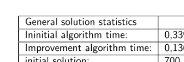
Ininitial algorithm time: 0,339394 Improvement algorithm time: 0,13691 initial solution: 700 improvement solution: 350
Table 4.2: General solution information of one instance
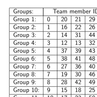
lem with team leaders and five chosen team members. In the example, the Greedy Matching algorithm and the Bipartite Weighted Matching Improve-ment algorithm apply. Table 4.1 and Table 4.2 show the obtained solution and results after completing the initial solution algorithm and running the improvement algorithm for 20 seconds respectively. Note that the algorithm does not find an improvement anymore after one second. The final observed answer has an overall penalty value that is equal to 350, meaning that one pair of students in the solution has been in the same team before. The penalty value after running the initial Greedy Matching algorithm is equal to 700. This is already relatively low, as we will see in a later stage of the chapter. Table 4.6 in the appendix shows the final group formations that led to the final penalty value of 350. The students with ID’s 0 up to 11 are team leaders and stay in group 1 up to 12 respectively, which explains why these are in this respective order in the table.
4.7.3
Empirical results on the initial solutions
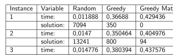
Instance Variable Random Greedy Greedy Matching 1 time: 0,011888 0,36688 0,429436
solution: 7094 350 0
2 time: 0,0147 0,350464 0,404976 solution: 13241 800 94 3 time: 0,014776 0,380394 0,437576
solution: 7588 397 47
Table 4.3: This table shows some data
algorithm to create a feasible solution is stable and quick over different in-stances. There is a small difference in running time between the two greedy algorithms, which implies that the individual bipartite matching problems find the answer very quickly. Overall, there is a preference for the third al-gorithm. However, as our implementation of this algorithm is dependent on external libraries that could cause implementation issues when implemented in current applications on other systems, the standard greedy algorithm is a good alternative that still establishes a feasible solution with a relatively low penalty value.
4.7.4
Empirical results on the improvement algorithms
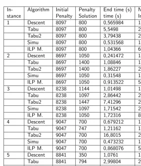
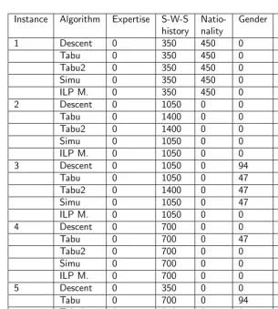
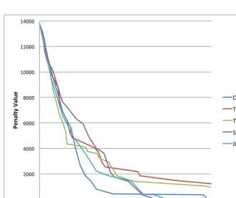
In order to test the improvement algorithms, the simulator generates differ-ent instances. Furthermore, we test instances with fewer or more predeter-mined team members/leaders. Table 4.4 presents the solutions generated by the different algorithms. Table 4.5 shows for each of the determined overall penalty values, how they are built up regarding the soft constraints. The instances on which the algorithms are applied contain both team lead-ers and five team memblead-ers. Additionally, Figure 4.2 shows the performance over time for the fifth instance of Table 4.4.
sec-4.7. COMPUTATIONAL RESULTS 129
0 1000 2000 3000 4000 5000 6000 7000 8000 9000
-‐0,1 0,1 0,3 0,5 0,7 0,9 1,1 1,3 1,5
Pen
al
ty
Va
lu
e
Time (seconds)
Descent Tabu1 Tabu2 Simu ILP M.
Figure 4.2: Module problem with group leaders and members Instance 5
onds, makes the ILP improvement algorithm the most preferred algorithm according to us. Next to the ILP matching algorithm, Simulated Annealing performs surprisingly well. Simulated Annealing together with Descent Im-provement finish often quicker than the ILP algorithm does. However, as the penalty values of the obtained solutions are sometimes higher on the same instance, these algorithms are not as effective as the Bipartite Weighted Matching algorithm. Descent Improvement and Simulated Annealing per-form relatively similar.
linkages persist that could cause conflicts that could not be solved. Both Tabu Searches only differing in their neighborhood are shown In Table 4.4 and Table 4.5, Tabu 1 corresponds to the Tabu Search algorithm using the ”Worst Performing Swap Neighborhood, whereas Tabu 2 uses the General Swap Neighborhood. From the implemented Tabu Search algorithms, Tabu 2 performs overall better, but still underperforms compared to the other im-provement algorithms. The first Tabu Search algorithm more likely causes sub-optimal answers than the second Tabu Search algorithm. For example, in later stages of the algorithm, when no direct improvements are found in the neighborhood, making swaps to the worsted performing groups may not lead to improvements, while other swaps between groups that are both not the worsted performing group could still improve the algorithm directly.
Table 4.5 showes that the constraint regarding the level of expertise is always optimally satisfied, given that the penalty value for all instances is equal to zero. Secondly, the constraint taking into account the student-with-student histories is the constraint that overall causes the largest increase in the penalty value. Very important to mention is that often these partly penalty values cannot be further decreased, as these penalties are often caused by pairs of students that have to be together in the same group.
4.7.5
Empirical results residential weeks
4.8. CONCLUSION 131
4.7.6
Overall evaluation of the program
Overall, it is observed that both the improvement algorithms and the ini-tial solution algorithms are helpful in solving the MBA sectioning problem at the SBE. Three of the four improvement algorithms seem to diminish the overall penalty value rapidly, while staying feasible. This includes both the regular module problem and the residential week problem. The perfor-mance of the algorithms on the module and residential week problem are very similar. In the previous sections, where we tested the improvement algorithms, initial solutions were generated by the random initial solution algorithm. However, the actual performance of combining the two type of algorithms is noticeable in Section 7.2, which showed the solutions from the algorithm combination including the Greedy Matching algorithm and the Bi-partite Matching Improvement algorithm. In this instance, the improvement algorithm only found one improvement.
Overall, given the different problem instances, and assuming that the simulation is correctly representing a real life example, the Bipartite Match-ing Improvement algorithm makes its last improvement always within three seconds and produces a solution that is at least as good as the other rithms. For this reason, it is determined to be the best improvement algo-rithm choice. Similarly, the Greedy Matching algoalgo-rithm is the best choice for creating an initial feasible solution for the MBA sectioning problem at SBE.
4.8
Conclusion
value is equal to the value from the best performing algorithm on any in-stance. The second applied method, Tabu Search, is a heuristic that forces a swap at every iteration. This swap in the specified neighborhood either leads to an improvement of the overall penalty value, or makes the swap that leads to the smallest worsening of the overall penalty value, taking into account the Tabu list. Although it was expected to obtain better results with Tabu Search, other algorithms resulted in better solutions. The next heuristic, Simulated Annealing, is as the previous two algorithms a Local Search algorithm. It makes guaranteed swaps when the best possible swap corresponds to an improvement of the overall penalty value, while it makes swaps with a probabilistic character if the swap does not lead to an improve-ment. This probability depends on how large the worsening of the specified swap is. The final discussed algorithm, the Bipartite Weighted Matching Improvement algorithm, iteratively selects students from groups, and finds local optimal solutions for a bipartite matching problem in order to improve the overall penalty value of the whole problem.
4.9. FURTHER RESEARCH 133
4.9
Further Research
In- Algorithm Initial Penalty End time (s) Nr. of stance Penalty Solution time (s) Impr.
1 Descent 8097 800 0,565984 15
Tabu 8097 800 5,5498 20
Tabu2 8097 800 3,79438 22
Simu 8097 800 0,531568 18
ILP M. 8097 800 1,04366 6
2 Descent 8697 1050 0,241472 14
Tabu 8697 1400 1,08846 19
Tabu2 8697 1400 1,86227 21
Simu 8697 1050 0,31548 13
ILP M. 8697 1050 0,913522 5
3 Descent 8238 1144 1,01498 15
Tabu 8238 1097 2,86442 21
Tabu2 8238 1447 7,41296 23
Simu 8238 1097 1,71542 20
ILP M. 8238 1050 1,72316 8
4 Descent 9047 700 0,679212 18
Tabu 9047 747 1,21162 17
Tabu2 9047 700 16,8015 27
Simu 9047 700 0,473232 16
ILP M. 9047 700 0,868076 5
5 Descent 8841 350 1,0761 17
Tabu 8841 794 2,99804 25
Tabu2 8841 350 2,62812 21
Simu 8841 350 1,29188 16
ILP M. 8841 350 0,995248 5
4.9. FURTHER RESEARCH 135
Instance Algorithm Expertise S-W-S Natio- Gender Total: history nality
1 Descent 0 350 450 0 800
Tabu 0 350 450 0 800
Tabu2 0 350 450 0 800
Simu 0 350 450 0 800
ILP M. 0 350 450 0 800
2 Descent 0 1050 0 0 1050
Tabu 0 1400 0 0 1400
Tabu2 0 1400 0 0 1400
Simu 0 1050 0 0 1050
ILP M. 0 1050 0 0 1050
3 Descent 0 1050 0 94 1144
Tabu 0 1050 0 47 1097
Tabu2 0 1400 0 47 1447
Simu 0 1050 0 47 1097
ILP M. 0 1050 0 0 1050
4 Descent 0 700 0 0 700
Tabu 0 700 0 47 747
Tabu2 0 700 0 0 700
Simu 0 700 0 0 700
ILP M. 0 700 0 0 700
5 Descent 0 350 0 0 350
Tabu 0 700 0 94 794
Tabu2 0 350 0 0 350
Simu 0 350 0 0 350
ILP M. 0 350 0 0 350
Bibliography
[1] E. H. E. H. L. Aarts and J. K. Lenstra. Local Search in Combinatorial Optimization. Princeton University Press, 2003.
[2] H. J. Bandelt, Y. Crama, and F.C.R. Spieksma. Approximation algo-rithms for multi-dimensional assignment problems with decomposable costs. Discrete Applied Mathematics, 49(1-3):25 – 50, 1994. Special Volume Viewpoints on Optimization.
[3] R. E. Burkard and E C¸ela. Linear assignment problems and extensions, 1998.
[4] E. K. Burke and S. Petrovic. Recent research directions in automated timetabling. European Journal of Operational Research, 140:266–280, 2002.
[5] M. W. Carter. A comprehensive course timetabling and student scheduling system at the university of waterloo. In Selected papers from the Third International Conference on Practice and Theory of Automated Timetabling III, PATAT ’00, pages 64–84, London, UK, UK, 2001. Springer-Verlag.
[6] M. W. Carter and G. Laporte. Recent developments in practical exami-nation timetabling. In Edmund Burke and Peter Ross, editors,Practice and Theory of Automated Timetabling, volume 1153 ofLecture Notes in Computer Science, pages 1–21. Springer Berlin Heidelberg, 1996. [7] M. W. Carter and G. Laporte. Recent developments in practical course
timetabling. In Edmund Burke and Michael Carter, editors, Practice and Theory of Automated Timetabling II, volume 1408 of Lecture Notes in Computer Science, pages 3–19. Springer Berlin Heidelberg, 1998.
[8] T. A. Feo and M. Khellaf. A class of bounded approximation algorithms for graph partitioning. Networks, 20(2):181–195, 1990.
[9] H. W. Kuhn. The hungarian method for the assignment problem.Naval Research Logistics Quarterly, 2(1-2):83–97, 1955.
[10] M. Marte.Models and Algorithms for School Timetabling. PhD thesis, Oktober 2002.
[11] T. Muller. Constraint-based Timetabling. PhD thesis, Charles Univer-sity Prague, Faculty of Mathematics and Physics, 2005.
[12] T. Muller and K. Murray. Comprehensive approach to student section-ing. Annals of Operations Research, 181(1):249–269, 2010.
[13] K. Murray, T. Muller, and H. Rudov´a. Modeling and solution of a complex university course timetabling problem. InPractice And Theory of Automated Timetabling, Selected Revised Papers, pages 189–209, 2007.
[14] W. R. Pulleyblank. Edmonds, matching and the birth of polyhedral combinatorics. Documenta Mathematica, Optimization Stories(Extra Volume):181–197, 2012.
[15] A Schaerf. A survey of automated timetabling. ARTIFICIAL INTEL-LIGENCE REVIEW, 13(2):87–127, 1999.
4.10. APPENDIX 139
4.10
Appendix
Groups: Team member ID’s Group 1: 0 20 21 29 47 Group 2: 1 16 22 26 58 Group 3: 2 14 31 44 53 Group 4: 3 12 13 32 56 Group 5: 4 37 39 43 45 Group 6: 5 38 41 48 59 Group 7: 6 27 36 40 54 Group 8: 7 19 30 46 55 Group 9: 8 28 42 49 52 Group 10: 9 15 18 25 34 Group 11: 10 17 23 50 51 Group 12: 11 24 33 35 57
0 2000 4000 6000 8000 10000 12000 14000
0 0,2 0,4 0,6 0,8 1 1,2 1,4
Pen
al
ty
Va
lu
e
Time (seconds)
Descent Tabu1 Tabu2 Simu ILP M.