C. Dobrzynski, T. Colin & R. Abgrall, Editors
IMPLEMENTATION OF OPTIMAL GALERKIN AND COLLOCATION
APPROXIMATIONS OF PDES WITH RANDOM COEFFICIENTS
∗,∗∗J. Beck
1, F. Nobile
2, L. Tamellini
2and R. Tempone
1Abstract. In this work we first focus on the Stochastic Galerkin approximation of the solutionuof an elliptic stochastic PDE. We rely on sharp estimates for the decay of the coefficients of the spectral expansion ofuon orthogonal polynomials to build a sequence of polynomial subspaces that features
better convergence properties compared to standard polynomial subspaces such as Total Degree or Tensor Product.
We consider then the Stochastic Collocation method, and use the previous estimates to introduce a new effective class of Sparse Grids, based on the idea of selecting a priori the most profitable hierarchical surpluses, that, again, features better convergence properties compared to standard Smolyak or tensor product grids.
Key words: Uncertainty Quantification, PDEs with random data, elliptic equations, multivariate polynomial approximation, BestM-Terms approximation, Stochastic Galerkin methods, Smolyak
ap-proximation, Sparse grids, Stochastic Collocation methods.
AMS Subject Classification: 41A10, 65C20, 65N12, 65N35
Introduction
Many works have been recently devoted to the analysis and the improvement of the Stochastic Galerkin and Collocation techniques for Uncertainty Quantification for PDEs with random input data. These methods are promising since they can exploit the possible regularity of the solution with respect to the stochastic parameters to achieve much faster convergence than sampling methods like Monte Carlo.
Stochastic Galerkin and Collocation methods can be classified asparametric techniques, since both expand u, the solution of the PDE of interest, as a summation over suitable deterministic basis functions in probability space, typically polynomials or piecewise polynomials. Stochastic Galerkin is a projection technique over a set of orthogonal polynomials with respect to the probability measure at hand (see e.g. [1, 12, 15, 20]), while Stochastic Collocation is a sum of Lagrangian interpolants over the probability space (see e.g. [2, 10, 22]).
∗ The authors would like to recognize the support of the PECOS center at ICES, University of Texas at Austin (Project Number 024550, Center for Predictive Computational Science). Support from the VR project ”Effektiva numeriska metoder f¨or stokastiska differentialekvationer med till¨ampningar” and King Abdullah University of Science and Technology (KAUST) is also acknowledged.
∗∗ The second and third authors have been supported by the Italian grant FIRB-IDEAS “Advanced numerical techniques for uncertainty quantification in engineering and life science problems”
1 Applied Mathematics and Computational Science, KAUST, Saudi Arabia, e-mail:[email protected],
2 MOX, Department of Mathematics “F. Brioschi”, Politecnico di Milano, Italy, e-mail:[email protected],
c
EDP Sciences, SMAI 2011
The comparison between performances of these deterministic methods is a matter of study (see e.g. [3]). However, both suffer the so-called “Curse of Dimensionality”: using naive projections/interpolations over tensor product polynomials spaces/tensor grids leads to computational costs that grow exponentially fast with the number of input random variables. In such a case, careful construction of approximation spaces/sparse grids is needed in order to retain accuracy while keeping computational work acceptably low.
In a Stochastic Galerkin setting this requirement can be translated to the implementation of algorithms able to compute what is known as “BestM-Terms approximation”. In other words, the method should be able to establish a-priori the set of theM most fruitful multivariate polynomials in the spectral approximation of the solutionu, and to compute only those terms.
Important contributions in the study of the BestM-Terms approximation have been given by Cohen, DeVore and Schwab: estimates on the decay of the coefficients of the spectral expansion of u have been proved e.g. in [6, 8, 9]. In this work we will reformulate and slightly generalize the result given in [9, Corollary 6.1], and show on few numerical examples that the sequence of polynomial subspaces built upon those estimates (“TD with Factorial Correction” sets, TD-FC in the following) performs better than classical choices such as Total Degree or Tensor Product in terms of error versus the dimension of the polynomial space.
In a Stochastic Collocation setting, the construction of an optimal grid can be recast into a classical knapsack problem relying on the notion of profit of each hierarchical surplus composing the sparse grid, as introduced e.g. in [7, 13] for approximation ofHr
mix functions. The “BestM-Terms” grid is then the one built with the set of theM most profitable hierarchical surpluses. In this work we provide a heuristic a-priori estimate of the profit of each hierarchical surplus, and use it to build a quasi optimal sparse grid. The estimates of the profit are in turn based on the estimates of the decay of the spectral expansion of u. Numerical investigations show that these new grids perform better than standard Smolyak grids as well as grids constructed with the dimension adaptive approach developed in [11, 14].
The paper is organized as follows. Section 1 defines the elliptic model problem of interest and gives general regularity results of the solution u. In Section 2 we first address the general procedure that leads to the Stochastic Galerkin approximation ofu; next we state the estimate for the decay of the spectral approximation ofuand explain how to build practically the TD-FC polynomial subspaces that stem from it. In Section 2.2 we consider some simple numerical tests where we can build explicitly the BestM-Terms approximation, and we compare it with the TD-FC and with some standard choices of polynomial subspaces. Finally, the construction of the approximated optimal sparse grids and their numerical testing are presented in Section 3.
1.
Problem setting
LetDbe a convex bounded polygonal domain inRdand (Ω,F, P) be a complete probability space. Here Ω is
the set of outcomes,F ⊂2Ωis theσ-algebra of events andP :F →[0,1] is a probability measure. Consider the
stochastic linear elliptic boundary value problem: find a random function,u:D×Ω→R, such thatP-almost
everywhere in Ω, or in other words almost surely (a.s.), the following equation holds:
(
−div(a(x, ω)∇u(x, ω)) =f(x) x∈D,
u(x, ω) = 0 x∈∂D. (1)
where the operators div and∇ imply differentiation with respect to the physical coordinatex only. We make the following assumptions on the random diffusion coefficient:
Assumption 1.1. a(x, ω) is strictly positive and bounded with probability 1, i.e. there exist amin > 0 and
amax<∞such thatP(amin≤a(x, ω)≤amax,∀x∈D) = 1.
Observe that Assumption 1.2 is not that restrictive. Indeed one could assume that ais parametrized by a non uniform random vector zand introduce a smooth non linear map y = Θ(z) that transforms the original variables into i.i.d. uniform variables.
We denote by Γn = (−1,1) the image set of the random variable yn, and Γ = Γ1×. . .×ΓN. After Assumption 1.2 the random vector y has a joint probability density function ρ : Γ → R+ that factorizes as
ρ(y) =QNn=1ρn(yn), ∀y ∈Γ, withρn = 12. Moreover, the solution uof (1) depends on the single realization
ω ∈Ω only through the value taken by the random vector y. We can therefore replace the probability space (Ω,F, P) with (Γ, B(Γ), ρ(y)dy), where B(Γ) denotes the Borelσ-algebra on Γ andρ(y)dyis the distribution measure of the vector y. We denote with L2
ρ(Γ) the space of square integrable functions on Γ with respect to the measure 1
2Ndy.
The assumption of independence of the random variables is very convenient for the development of the techniques proposed below, since they rely on tensor polynomial approximations. However, such assumption is not essential and could be removed whenever the density ρ does not factorize, by introducing an auxiliary density ˆρ = 1
2N as suggested in [2]. The price to pay in the convergence estimate is then a costant factor
proportional tokρ/ρˆkL∞(Ω).
In the rest of the paper we will use the following notation: given a multi-indexi∈NN and a vectorr∈RN,
we define |i| = PNn=1in, i! = QNn=1(in!) and ri = QNn=1rinn. We can now state a regularity assumption on
a(x,y):
Assumption 1.3. a(x,y)is infinitely many times differentiable with respect toyand∃r∈RN
+,r= [r1, ..., rN]
independent of yandis.t.
∂ia
a (y)
L∞
(D) ≤ri
∀y∈Γ,
whereiis a multi-index in NN,∂ia= ∂
i1+...+iNa
∂yi1
1 · · ·∂yiNN
.
Remark 1.4. A common situation of interest is whena(x, ω) is an infinitely dimensional random field, suitably expanded in series (e.g. by a Karh`unen-Lo`eve or Fourier expansion) either as alinear expansion of the form a=a0+P∞n=1bn(x)ynor anexponential expansion of the forma=a0+ exp (P∞n=1bn(x)yn), withbn∈L∞(D) in both cases. Then the infinite series is truncated up to N terms, with N large enough to take into account a sufficient amount of the total variability. Both expansions comply with the previous assumption with rn = kbnkL∞(D)/aminand rn =kbnkL∞(D), respectively.
Finally, we denote by V = H1
0(D), the space of square integrable functions in D with square integrable
distributional derivatives and with zero trace on the boundary, equipped with the gradient norm kvkV = k∇vkL2(D),∀v ∈ V. Its dual space will be denoted by V′. We are now in the position to write a weak formulation of problem (1):
Weak Formulation. Find u∈V⊗L2
ρ(Γ) such that∀v∈V⊗L2ρ(Γ) Z
Γ Z
D
a(x,y)∇u(x,y)· ∇v(x,y)ρ(y)dxdy=
Z
Γ Z
D
f(x)v(x,y)ρ(y)dxdy. (2) Under Assumption 1.1, a straightforward application of the Lax-Milgram lemma yields that there exists a unique solution to problem (2) for anyf ∈V′. Moreover, the following estimate holds:
kukV⊗L2
ρ(Γ)≤
kfkV′
amin .
Concerning the regularity of the solution with respect toy, under Assumptions 1.1 - 1.3 the following result is proved in [5].
which implies that uis analytic in every y∈Γ. HereC0= kfkV
′
amin and ˜r= 3
2r, with ras in Assumption 1.3. A
similar result is given in [9] for the special casea=a0+PNn=1bn(x)yn.
2.
Stochastic Galerkin method
We now seek an approximation of the solution uwith respect to y by global polynomials. As anticipated in the introduction, we remark that the choice of the polynomial space is critical when the number N of input random variables is large, since the number of stochastic degrees of freedom might grow very quickly withN, even exponentially when isotropic tensor product polynomial spaces are used (see Table 1). This effect is known as thecurse of dimensionality.
Several choices of polynomial spaces that mitigate this phenomenon have been proposed in the literature, see e.g. [3]. In this work we consider a general multivariate space: letw∈Nbe an integer index denoting the level
of approximation andp= (p1, . . . , pN) a multi-index. Let Λ(w) be a sequence of increasing index sets such that Λ(0) ={(0, . . . ,0)}and Λ(w)⊆Λ(w+ 1)⊂NN, forw≥0. We introduce the multivariateρ(y)dy-orthonormal
Legendre polynomialsLp(y) =QNn=1Lpn(yn), whereLpn(t) are the monodimensional Legendre polynomials of
degreepn, and consider the multivariate polynomial subspace ofL2ρ(Γ) built as
PΛ(w)(Γ) =span{Lp(y) withp∈Λ(w)}.
We then seek an approximationuw∈V⊗PΛ(w)(Γ). Table 1 shows common choices for Λ(w).
index set Λ(w) Dimension|Λ(w)| Tensor product space (TP) {p∈NN : maxn=1...,Npn≤w} (1 +w)N
Total degree space (TD) {p∈NN : PN
n=1pn≤w}
N+w N
Hyperbolic cross space (HC) {p∈NN : QNn=1(pn+ 1)≤w+ 1} ≤(w+ 1) (log (e(w+ 1) ) )N−1 Table 1. Common polynomial spaces. The result for HC is only an upper bound.
For further details on these spaces, see [3] and references therein. In [3] we have also considered anisotropic versions of these spaces as in Table 2, where α = (α1, . . . , αN) ∈ RN
+ is a vector of positive weights and
αmin= minnαn.
Tensor product space (TP) Λ(w) ={p∈NN : maxn=1...,Nαnpn ≤αminw}
Total degree space (TD) Λ(w) ={p∈NN : PN
n=1αnpn≤αminw} Hyperbolic cross space (HC) Λ(w) ={p∈NN : QN
n=1(pn+ 1)
αn
αmin ≤w+ 1}
Table 2. Anisotropic version of polynomial spaces
We can interpret these weights as a measure of the importance of each random variable yn on the solution: the smaller the weight, the higher degree we allow in the corresponding variable. The Stochastic Galerkin (SG) approximation then consists in restricting the weak formulation (2) to the subspace V⊗PΛ(w)(Γ) and reads:
Galerkin Formulation. Find uw∈V⊗PΛ(w)(Γ)such that ∀vw∈V⊗PΛ(w)(Γ) Z
Γ Z
D
a(x,y)∇uw(x,y)· ∇vw(x,y)ρ(y)dxdy= Z
Γ Z
D
f(x)vw(x,y)ρ(y)dxdy. (3)
Now let φ(x) be a basis function for the physical space V. Inserting vw = φ(x)Lq(y) with q ∈ Λ(w) as
test function in the weak formulation (3) will result in a set of equations in weak form for the coefficients up(x) that will be generally coupled due to the presence in the equation (3) of the terma(x,y)Lp(y)Lq(y). See
e.g. [3,17,18] for further details on space discretization and on the numerical solution of the system of equations.
2.1.
Optimal choice of polynomial spaces
The question that naturally arises in the context of Galerkin approximation concerns the best choice of the polynomial space to be used, to get maximum accuracy for a given dimension M of the space (Best M -Terms approximation). Let us assume the solution u(x,y) is known and consider its expansion on Legendre polynomials,
u(x,y) = X
p∈NN
up(x)Lp(y), up(x) = Z
Γ
u(x,y)Lp(y)ρ(y)dy.
We look for an index set S ⊂NN with cardinalityM that minimizes the error
ku−X
p∈S
upLpk2V⊗L2
ρ(Γ)= X
p∈S/ ||up||2V
where the equivalence is a consequence of Parseval’s equality. The obvious solution to this problem is the setS that contains theM coefficientsupwith largest norm. This solution of course is not constructive; what we need
are sharp estimates of the decay of the coefficientskupkV, based only on computable quantities, to be used in
the approximation of the setS.
Seminal works in this direction are [6, 8, 9], where estimates of the decay of the Legendre coefficients are provided. We consider here a slight generalization of the result in [9, Corollary 6.1] and show numerically that the polynomial sets, hereafter called TD-FC (“TD with Factorial Correction”), built on these modified estimates behave closely to the real BestM-Terms approximation.
Under Assumptions 1.1 - 1.3 it is possible to prove that the following estimate holds for the Legendre coefficients:
kupkV≤C0e−
P
ngnpn|p|!
p! (4)
withgn=−log rn/ √3 log 2andrn as in Assumption 1.3. For a proof of (4) see [5]. Again, a similar result is given in [9] for the special casea=a0+PNn=1bn(x)yn.
We define now the sequence of TD-FC sets, with increasing approximating accuracy, by selecting all multi-indicespfor which theestimated decay of the corresponding Legendre coefficient, given in (4), is above a fixed thresholdǫ. This, in turn, corresponds to selecting those indicespsuch that
e−PNn=1gnpn|p|!
p! ≥ǫ ⇐⇒ −
N X
n=1
gnpn+ log| p|!
p! ≥logǫ. The TD-FC sets are then defined as
Λ(w) =
(
p∈NN :
N X
n=1
gnpn−log|p|! p! ≤w
)
(5)
withw∈N+=⌈−logǫ⌉. The quantitiesgn=−log rn/ √3 log 2appearing in (5) can be estimateda-priori
unsatisfactory; on the other hand it is found that bound (4) works particularly well if the ratesgn are estimated numerically rather thana-priori, as the following numerical results will show. To estimate numericallygn, one increases the polynomial degree in one random variable at a time while keeping degree zero in all the others variables and estimate numerically the exponential rate of convergence. Observe that in such monovariate analyses the factorial term does not appear so the expected convergence rate is precisely ∼e−gnpp.
Remark 2.1. Observe that Λ(w) actually depends onN but one can extend this also to the case wherepis a sequence of natural numbers (“infinite dimensions multi-indices”) with only a finite number of non zero terms, providedgn →+∞asn→ ∞. This is an alternative way to work with random fields, without truncating them a priori to a certain level (see e.g. [8, 16]).
2.2.
Numerical Tests
In this section we show the performance of the TD-FC sets (5) compared to the isotropic and anisotropic versions of TD sets defined in Tables 1 and 2 as well as the Best M-Terms approximation. We consider the following elliptic problem in one physical dimension
(
−(a(x,y)u(x,y)′)′= 1 x∈D= (0,1), y∈Γ
u(0,y) =u(1,y) = 0, y∈Γ (6) with different choices of diffusion coefficienta(x,y), for which Assumptions 1.1 - 1.3 hold. We focus on a linear functionalψ: V→R, so thatψ(u) is a scalar random variable, function ofyonly. In our examples,ψis defined
as ψ(v) =v(1 2).
To obtain the BestM-Terms approximation we compute explicitly all the Legendre coefficients of ψ(u) in a sufficiently large index setU, evaluating the integrals ψp=R
Γψ(u)Lp(y)ρ(y)dy with a high-level sparse grid.
We order then the coefficients in decreasing order, according to their V norm and take the partial sums of the reordered sequence as the BestM-Terms approximation. The ratesgused to build the TD-FC space, as well as the anisotropic TD space (withαn =gn), are computed numerically as explained in the previous Section.
Test 1: diffusion coefficient depending on 2 random variables
The first case we consider has two random variables (y1, y2) and a diffusion coefficienta(x,y) = 1 + 0.1xy1+
0.5x2y
2; results are shown in Figure 1.
Figure 1(a) shows the Legendre coefficients ordered in lexicographic order, giving this peculiar sawtooth shape. The first tooth corresponds to multi-indices of the form [0, k], the second one to [1, k] and so on. We have also added to the plot the estimate (4) of the magnitude of the Legendre coefficients, which leads to the TD-FC sets (5), as well as the estimate |ψp| ≤ C0e−
P
ngnpn, where the factorial terms have been dropped,
which leads to the anisotropic TD spaces. The plot suggests that estimate (4) is quite sharp, whereas the estimate corresponding to the TD space underestimates considerably the Legendre coefficients. This highlights the importance of the factorial term in (4). We expect, therefore, that the TD-FC approximation performs better than the aniso-TD one. Moreover, we point out the non intuitive fact that the Legendre coefficientsψp are not strictly decreasing in absolute value in the lexicographic order. As an example,|ψ[5 0]|<|ψ[5 1]|, and the
same holds for all teeth but the first few.
Figure 1(b) shows convergence plots for the error in L2
0 20 40 60 80 100 10−20
10−18 10−16 10−14 10−12 10−10 10−8 10−6 10−4
10−2 Legendre coeffTD appr TD−FC appr
(a) Legendre coefficients in lexicographic order and their corre-sponding estimates based on either TD-FC or TD approxima-tions.
0 20 40 60 80
10−9 10−8 10−7 10−6 10−5 10−4 10−3 10−2 10−1
best M term TD
iso−TD TD−FC
(b) Convergence of different polynomial approximations, mea-sured askψ(u)−ψ(uw)kL2
ρ(Γ)versus dimension of polynomial space
Figure 1. Results for a(x,y) = 1 + 0.1xy1 + 0.5x2y2. Here we have g ≃ (2.96,1.57),
U =TP(12), Legendre coefficients computed with a standard Smolyak sparse grid of level 9,
with Gauss-Legendre abscissae.
0 20 40 60 80 100 120 10−10
10−9 10−8 10−7 10−6 10−5 10−4 10−3 10−2
best M term TD
iso−TD TD−FC
Figure 2. Results fora(x,y) = 4 +y1+ 0.2 sin(πx)y2+ 0.04 sin(2πx)y3+ 0.008 sin(3πx)y4.
Here we have g ≃ (2.035,4.11,5.73,7.05), U =TD(9). The convergence is measured by
kψ(u)−ψ(uw)kL2
ρ(Γ) versus the dimension of the polynomial space.
Test 2: diffusion coefficient depending on 4 random variables
We now considera(x,y) = 4+y1+0.2 sin(πx)y2+0.04 sin(2πx)y3+0.008 sin(3πx)y4, and look at the functional
3.
Stochastic Collocation
The Stochastic Collocation (SC) Finite Element method consists in collocating problem (1) in a set of points {yj∈Γ, j= 1, . . . , Mw}, i.e. computing the corresponding solutionsu(·,yj) and building a global polynomial approximation uw, not necessarily interpolatory, upon those evaluations: uw(x,y) = PMj=1wu(x,yj) ˜ψj(y) for suitable multivariate polynomials{ψ˜j}Mw
j=1.
Building the set of evaluation points{yj} as a cartesian product of monodimensional grids becomes quickly unfeasible since the computational cost grows exponentially fast with the number of stochastic dimensions needed. We consider instead the so-called sparse grid procedure, originally introduced by Smolyak in [19] for high dimensional quadrature purposes; see also [4, 7] for polynomial interpolation. In the following we briefly review and generalize this construction.
For each direction yn we introduce a sequence of one dimensional polynomial interpolant operators of in-creasing order: Unm(i) : C0(Γn)→ Pm(i)−1(Γn). Here i ≥1 denotes the level of approximation and m(i) the number of collocation points used to build the interpolation at level i. As a consequence,Unm(i)[q] =qifqis a polynomial of degree up tom(i)−1. We require the functionmto satisfy the following assumptions: m(0) = 0, m(1) = 1 andm(i)< m(i+ 1) fori≥1. In addition, letU0
n = 0,∀q∈C0(Γn).
Next we introduce the difference operators ∆mn(i)=Unm(i)−Unm(i−1), an integer valuew≥0 and a sequence of index setsI(w) such thatI(w)⊂ I(w+ 1) andI(0) ={(1,1, . . . ,1)}. We define the sparse grid approximation ofu(y) : Γ→V at levelwas
uw(y) =SIm(w)[u](y) = X
i∈NN
+:i∈I(w) N O
n=1
∆m(in)
n [u](y). (7)
The set of all evaluation points needed is calledsparse grid and denoted by Hm
I(w)⊂Γ. To fully characterize
the sparse approximation operatorSIm(w)one has to provide the sequence of setsI(w), the relation between the
level iand the number of points m(i) in the corresponding one dimensional polynomial interpolation formula Um(i), and the family of points to be used at each level, e.g. Clenshaw-Curtis or Gauss abscissae (see e.g. [21]). Remark 3.1. As pointed out in [11], the sparse approximation is well defined only if the sum (7) is actually a telescopic sum. This is not ensured by any arbitrary I, and we have to pose some additional constraints onI. Following [11] we say that a setI isadmissible if for all i∈ I
i−ej∈ I for 1≤j≤N, ij >1. (8) We refer to this property asadmissibility condition, orADM in short. Given a setI we will denote byIADM the smallest set such thatI ⊂ IADM and IADM is admissible.
In what follows we will consider Clenshaw-Curtis abscissae and the “doubling” rulem(i) =db(i) = 2i−1+ 1,
which leads to nested grids. The classical Smolyak sparse grid (SM) usesI(w) ={i∈N+N :|i−1| ≤w}, which
clearly satisfies the admissibility condition (8). A quasi optimal choice of I(w) will be discussed in the next Section.
3.1.
Quasi-optimal sparse grids
We now aim at constructing the quasi-optimal sparse grid for Stochastic collocation method, i.e. at choosing the best sequence of sets of indices. We will rely on the estimate (4) on the decay of the Legendre expansion of u.
To this end, let us define the error associated to a sparse grid asE(S) =u− Sm h,w[u]
V⊗L2
ρ(Γ)
, and the work
W(S) as the number of evaluations needed, i.e. W(S) =|Hm
of a multi-indexi. LetIbe any set of indices such thati∈ I/ and{I∪i}is admissible. Then the error contribution ofiis ∆E(i) =Sm
{I∪i}[u]− SIm[u]
V⊗L2
ρ(Γ)
and the work contribution is ∆W(i) =|W(Sm
{I∪i})−W(SIm)|.
Following [7, 11] we can define the profit of an indexias
P(i) = ∆E(i) ∆W(i)
and define the optimal sparse approximation operatorS∗ as the one using the set of most profitable indices, i.e.
I∗(ǫ) ={i∈NN
+ :P(i)≥ǫ}.
To build the setI we rely on estimates for both ∆E(i) and ∆W(i). Since using Clenshaw-Curtis abscissae and doubling rule db(·) we get nested grids, we can computeexactly ∆W(i) as
∆W(i) = N Y
n=1
(db(in)−db(in−1)). (9)
On the other hand an estimate of the error contribution ∆E(i) requires some additional effort. We conjecture that the decay of ∆E(i) is related to the decay of the Legendre coefficients, through the Lebesgue constant
L(m(i)) associated toNN
n=1U m(in)
n :
∆E(i)[u].um(i−1)
VL(m(i)), (10)
where a.b means that there exists a constant c independent of i such thata ≤cb, um(i−1) is the Legendre
coefficient associated to the multi-indexm(i−1), and for Clenshaw-Curtis abscissae with doubling relation the Lebesgue constant is
L(db(i))≤
N Y
n=1
2
πlog(db(in) + 1) + 1
.
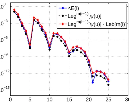
Figure 3 shows the decay of the error ∆E(i) and the corresponding m(i−1)-th Legendre coefficients for the quantity|ψ(u)|, whereu(x,y) solves problem (6) witha(x,y) = 1 + 0.1xy1+ 0.5x2y2, as in Section 2.2, Test 1.
These results, as well as the ones presented in the next Section, confirm that estimate (10) is accurate enough for our purposes.
Starting from (9) and (10), we can estimate the profit of each index, and estimate the sequence SI∗
(ǫ) of
quasi-optimal grids with
I∗(ǫ) =
i∈NN+ :
C0exp − N X
n=1
db(in−1)gn !
|db(i−1)|!
db(i−1)! L(db(i)) N
Y
n=1
(db(in)−db(in−1))
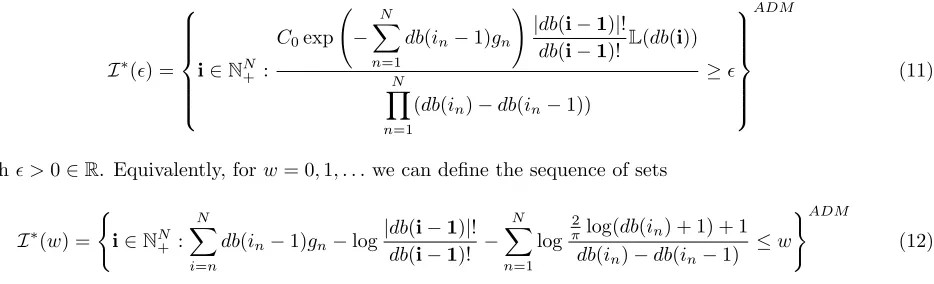
≥ǫ ADM (11)
withǫ >0∈R. Equivalently, forw= 0,1, . . . we can define the sequence of sets
I∗(w) =
(
i∈NN+ :
N X
i=n
db(in−1)gn−log|
db(i−1)|! db(i−1)! −
N X
n=1
log
2
πlog(db(in) + 1) + 1
db(in)−db(in−1) ≤w )ADM
(12)
0 5 10 15 20 25 30 10−15
10−12 10−9 10−6 10−3
100 ∆E(i)
Legm(i−1)[ψ(u)]
Legm(i−1)[ψ(u)] ⋅ Leb[m(i)]
Figure 3. Numerical comparison between ∆E(i),|ψ(u)m(i−1)|and estimate (10) forψ(u) as in
Section 2.2 Test 1. Both the ∆E(i) fori∈T P(4) and the corresponding Legendre coefficients |ψ(u)m(i−1)|have been computed with a standard sparse grid SM(10).
Remark 3.2. Observe that in definitions (11) and (12) the set has to be made admissible, as the condition on the multi-indices given inside the brackets might not satisfy ADM. This simply implies that if at level w an index j is added, all indicesi∈NN : i1≤j1, i2≤j2, . . . , iN ≤jN have to be added as well, if not already
present in the set.
3.2.
Numerical tests on sparse grids
In this Section we consider again problem (6) with the diffusion coefficientsa(x,y) as in Section 2.2 and use it to test the performance of the EW grids derived above, comparing them with the classical SM grid and the BestM-Terms approximation. The decay coefficientsgn in (12) are estimated numerically as in Section 2.2.
To approximate the BestM-Terms we again consider a sufficiently large setUof multi-indices and for each
of them we compute ∆W(i), ∆E(i) and their profit P(i). Next, we sort the multi-indices according to P(i), modify the sequence to fulfil the ADM condition (8) and compute the sparse grids according to this sequence. We remark that the procedure just described only leads to an approximation of the BestM-Terms solution. Indeed, on the one hand replacing the total errorE(S) with the sumPi∆E(i) provides only an upper bound that could be pessimistic because of possible cancellations, since the details ∆m(i)[u] are not mutually orthogonal,
in general. On the other hand the fact that the most profitable index may be not admissible suggests that the solution cannot be found using a greedy algorithm.
We also compare our results with the dimension adaptive algorithm proposed in [11], in the implementation of [14], available athttp://www.ians.uni-stuttgart.de/spinterp. This is an adaptive algorithm that given a sparse grid SI explores all neighbour multi-indices and adds to I the most profitable ones. The algorithm
implemented in [14] has a tunable parametereωthat allows one to move continuously from the classical Smolyak formula (ωe = 0) to the fully adaptive algorithm (ωe = 1). Following [14], in the present work we have set
e
ω = 0.9, that numerically has been proved to be a good performing choice. The cost of this algorithm is the
total number of evaluations needed, including also those necessary to explore all neighbours, to find the most profitable multi-index.
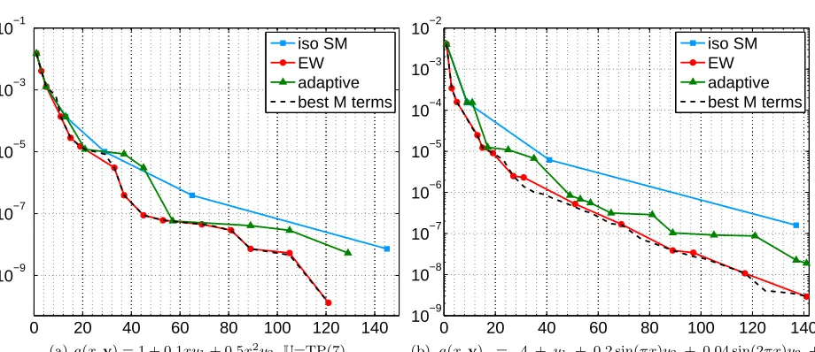
Figure 4 shows the convergence of the quantity kψ(u)−ψ(uw)kL2
ρ(Γ) versus the number of grid points, for
the different sparse grids considered. The L2
0 20 40 60 80 100 120 140 10−9
10−7 10−5 10−3 10−1
iso SM EW adaptive best M terms
(a)a(x,y) = 1 + 0.1xy1+ 0.5x2y2,U=TP(7)
0 20 40 60 80 100 120 140 10−9
10−8 10−7 10−6 10−5 10−4 10−3 10−2
iso SM EW adaptive best M terms
(b) a(x,y) = 4 +y1 + 0.2 sin(πx)y2 + 0.04 sin(2πx)y3 +
0.008 sin(3πx)y4,U=TD-FC (22)
Figure 4. Results for EW sparse grids compared with Best M-Terms , isotropic Smolyak and dimension adaptive algorithm. Convergence is measured in terms ofkψ(u)−ψ(uw)kL2(Γ) versus the number of evaluations (grid points).
4.
Conclusions
In this work we have proposed a new sequence of polynomial subspaces (TD-FC spaces in short) to be used in the solution of elliptic stochastic PDEs with Galerkin method, based on sharp estimates of the decay of the Legendre coefficients.
The performances of TD-FC spaces have been assessed through some simple test cases. Here we have compared TD-FC with some standard choices of polynomial spaces and with the BestM-Terms approximation of the solution, that can be explicitly built for the examples considered. Results show that the TD-FC spaces perform better than the anisotropic standard ones, and are close to the BestM-Terms approximation. However, the standard spaces may still have reasonable performances, if used in an appropriate anisotropic framework.
Using the estimate for the decay of the Legendre coefficients we have also defined a new class of sparse grids to be used in the context of Stochastic Collocation, relying on the concept of profit of each multi-index in the sparse grid. Again numerical tests suggest that these new sparse grids outperform the classical Smolyak construction, as well as the a-posteriori dimension adaptive algorithm as implemented in [14]. The reason for this apparent success is that our algorithm picks up the hierarchical surpluses based purely on a priori estimates and inexpensivey−one dimensional auxiliary problems. These estimates turn out to be quite sharp, and do not have any extra cost to explore neighbor points as the algorithm in [14] does.
References
[1] I. M. Babuˇska, R. Tempone, and G. E. Zouraris. Galerkin finite element approximations of stochastic elliptic partial differential equations.SIAM J. Numer. Anal., 42(2):800–825, 2004.
[2] I. Babuˇska, F. Nobile, and R. Tempone. A stochastic collocation method for elliptic partial differential equations with random input data.SIAM J. Numer. Anal., 45(3):1005–1034, 2007.
[3] J. B¨ack, F. Nobile, L. Tamellini, and R. Tempone. Stochastic spectral Galerkin and collocation methods for PDEs with random coefficients: a numerical comparison. In J.S. Hesthaven and E.M. Ronquist, editors,Spectral and High Order Methods for Partial Differential Equations, volume 76 ofLecture Notes in Computational Science and Engineering, pages 43–62. Springer, 2011. Selected papers from the ICOSAHOM ’09 conference, June 22-26, Trondheim, Norway.
[4] V. Barthelmann, E. Novak, and K. Ritter. High dimensional polynomial interpolation on sparse grids.Adv. Comput. Math., 12(4):273–288, 2000.
[5] J. Beck, F. Nobile, L. Tamellini, and R. Tempone. On the optimal polynomial approximation of stochastic PDEs by Galerkin and collocation methods. MOX-Report 2011-23, MOX - Department of Mathematics, Politecnico di Milano, 2011. To appear onMathematical Models and Methods in Applied Sciences.
[6] M. Bieri, R. Andreev, and C. Schwab. Sparse tensor discretization of elliptic sPDEs. SAM-Report 2009-07, Seminar f¨ur Angewandte Mathematik, ETH, Zurich, 2009.
[7] H.J Bungartz and M. Griebel. Sparse grids.Acta Numer., 13:147–269, 2004.
[8] A. Cohen, R. DeVore, and C. Schwab. Analytic regularity and polynomial approximation of parametric and stochastic elliptic PDEs. SAM-Report 2010-03, Seminar f¨ur Angewandte Mathematik, ETH, Zurich, 2010.
[9] A. Cohen, R. DeVore, and C. Schwab. Convergence rates of bestn-term Galerkin approximations for a class of elliptic sPDEs. Foundations of Computational Mathematics, 10:615–646, 2010. 10.1007/s10208-010-9072-2.
[10] B. Ganapathysubramanian and N. Zabaras. Sparse grid collocation schemes for stochastic natural convection problems.Journal of Computational Physics, 225(1):652–685, 2007.
[11] T. Gerstner and M. Griebel. Dimension-adaptive tensor-product quadrature.Computing, 71(1):65–87, 2003.
[12] R. G. Ghanem and P. D. Spanos.Stochastic Finite Elements: a Spectral Approach. Springer–Verlag, New York, 1991. [13] M. Griebel and S. Knapek. Optimized general sparse grid approximation spaces for operator equations. Math. Comp.,
78(268):2223–2257, 2009.
[14] A. Klimke.Uncertainty modeling using fuzzy arithmetic and sparse grids. PhD thesis, Universit¨at Stuttgart, Shaker Verlag, Aachen, 2006.
[15] H. G. Matthies and A. Keese. Galerkin methods for linear and nonlinear elliptic stochastic partial differential equations. Comput. Methods Appl. Mech. Engrg., 194(12-16):1295–1331, 2005.
[16] F. Nobile, R. Tempone, and C.G. Webster. An anisotropic sparse grid stochastic collocation method for partial differential equations with random input data.SIAM J. Numer. Anal., 46(5):2411–2442, 2008.
[17] M.F. Pellissetti and R.G. Ghanem. Iterative solution of systems of linear equations arising in the context of stochastic finite elements.Adv. Eng. Software, 31:607–616, 2000.
[18] C.E. Powell and H.C. Elman. Block-diagonal preconditioning for spectral stochastic finite-element systems.IMA J. Numer. Anal., 29(2):350–375, 2009.
[19] S.A. Smolyak. Quadrature and interpolation formulas for tensor products of certain classes of functions.Dokl. Akad. Nauk SSSR, 4:240–243, 1963.
[20] R. A. Todor and C. Schwab. Convergence rates for sparse chaos approximations of elliptic problems with stochastic coefficients. IMA J Numer Anal, 27(2):232–261, 2007.
[21] Lloyd N. Trefethen. Is Gauss quadrature better than Clenshaw-Curtis? SIAM Rev., 50(1):67–87, 2008.
[22] D. Xiu and J.S. Hesthaven. High-order collocation methods for differential equations with random inputs. SIAM J. Sci. Comput., 27(3):1118–1139, 2005.