Jean-Fr´ed´eric Gerbeau & St´ephane Labb´e, Editors
STOCHASTIC MATRICES AND
L
pNORMS : NEW ALGORITHMS FOR
SOLVING ILL-CONDITIONED LINEAR SYSTEMS OF EQUATIONS
Riadh Zorgati
1,2, Wim van Ackooij
2and Marc Lambert
1Abstract. We propose new iterative algorithms for solving a system of linear equations, possibly singular and inconsistent, presenting outstanding performances regarding ill-conditioning and error propagation. The basis of our approach is constructing with the l1 norm, a preconditioning matrix C (an approximation of a generalized inverse of the matrix) such that the preconditioned matrixCA is stochastic. This property allows us to retrieve, in an original way, the Schultz-Hotelling-Bodewig’s algorithm of iterative refinement of the approximate inverse of a matrix. The approach, valid for non-negative matrices, is then generalized to any complex, rectangular matrix. We are then able to compute a generalized inverse of any matrix and this inverse is fit for use in classical solving schemes such as : Richardson-Tanabe, Schultz-Hotelling-Bodewig, preconditioned conjugate gradients and also in the Kaczmarz scheme (that we have generalized usinglp norms). Regarding the obtained results on pathological well-known test-cases such as Hilbert and Nakasaka matrices, some of the proposed algorithms are empirically shown to be more efficient than the known classical techniques.
1.
Introduction
Consider any system of linear equations:
Ax=b, (1.1)
whereA is am×ncomplex matrix and xandb are complex vectors of dimensionsnandmrespectively.
When (1.1) is solvable, many methods of resolution can be implemented according to the characteristics of the matrix A. Considering for example, classical methods when A is square, the direct method of gaussian elimination or classical iterative methods as Jacobi or Gauss-Seidel are well-suited for providing precise solutions as long asAhas no pathological numerical features. IfAis hermitian, positive-definite, the conjugate gradients method of [7] is preferable. For rectangular, possibly singular systems, we can use projective methods of Kaczmarz [11] and Cimmino [5], who converge for any system with nonzero rows to the unique solution of a generalized solution if such solutions exist [1, 18].
1 Supelec, Plateau de Moulon, 3 rue Joliot-Curie, F-91192 Gif-sur-Yvette Cedex FRANCE. Tel: +33 (0)1 47 65 49 79; e-mail:[email protected] & [email protected]
2 EDF R&D. 1, avenue du G´en´eral de Gaulle, F-92141 Clamart Cedex FRANCE. Tel: +33 (0)1 47 65 58 31;
e-mail:[email protected] & [email protected]
c
Theoretically, solving (1.1) poses no difficulty. In practice, however it often meets with the snags of error propagation and ill-conditioning of the matrix A. The Gauss method, is particularly sensitive to these two challenges (for illustration of the error propagation snag, see for example [14] and [19]).
As (1.1) may have no classical solution, following [19], we consider solving the system
Ax=AA−b, (1.2)
instead of (1.1), which always has a solution x= A−b, whereA− is a generalized inverse of A. Considering (1.2) instead of (1.1) is justified by the fact that when (1.1) is solvable, the sets of solutions of (1.1) and (1.2) coincide due to the equalityAA−b=b which holds for any generalized inverseA− ofA.
Let us consider the system :
RAx=Rb, (1.3)
The matrixRis said to be a gain matrix ifRb∈Im(RA),ρ(I−RA|Im(I−RA))<1 whereρis the spectral radius of the iteration matrixQ=I−RA|Im(I−RA)and if furthermore Ker(RA) = Ker(A). LetS(H, y) be the set of all solutions of equationHx=y. IfR is a gain matrix, then equation (1.3) is solvable and the set of solutions of (1.2) coincides with the set of solutions of (1.3), i.e.,
S(A, AA−b) =S(RA, Rb).
Considering (1.2) instead of (1.1) and then considering (1.3) instead of (1.2) actually results in considering (1.1) preconditioned by a matrixR. The preconditioning matrixRis then chosen in a way to guarantee existence of a solution. Furthermore the choice is such that the computation of the solution from a numerical point of view is tractable.
For a given gain matrixR, three iterative schemes of resolution can be used for solving (1.3). Without considering stopping criteria for simplifying the presentation, these schemes are :
• the Richardson-Tanabe scheme :
x0∈Cn α∈i0, 2
ρ(RA)
i
F or k= 1,2, ...
xk+1 =xk+αR b−Axk
End f or
Such linear stationary iterative processes have been characterized by [19].
• the Schultz-Hotelling-Bodewig’s scheme of iterative refinement of the inverse of a matrix:
ρ I−RA|Im(I−RA)
<1 R0 =R
F or k= 1,2, ...
Rk+1=Rk 2I−ARk
End f or
• the Hestenes-Stiefel’s conjugate gradients scheme, for any matrixAhermitian, positive-definite :
x0 p0=r0=Rb−RAx0
F or k= 0,1, ... αk = krkk
2
hRApk,pki
xk+1=xk+α
kpk
rk+1 =rk−α
kRApk
βk+1=krk+1k
2
krkk2
pk+1=rk+1+βk+1pk
End f or
Many gain matrices may be chosen. Some of them are quite famous : the Jacobi matrix, defined if allaij are nonzero and convergent for any diagonally dominant matrixA:
R=
1
a11 0
1 aij
0 1
ann
= diag(A)−1=J
and the matrix R=αA∗, built using the adjoint matrixA∗, and convergent for any scalarαsatisfying:
0< α < 2 ρ(A∗A)
This matrix allows us to obtain the Moore-Penrose generalized inverse, calledP, and characterized byAP A=A,
P AP =P, (P A)∗ =P A, (AP)∗=AP. This means that the Moore-Penrose generalized inverse is a reflexive, a least-squares and a minimum norm generalized inverse.
In addition, we focus on two gain matricesR who are particularly interesting because they always satisfy the convergence conditionρ(I−RA|Im(I−RA))<1 for any nonzero row matrixA, as the matrix we will propose in this paper :
• the Kaczmarz-Tanabe matrix, calledK= [K1...Kn], with
Ki= 1
kaik22
i−1
Y
j=1
(I− 1 kajk22
a∗jaj)a∗i,
where the product is considered to beI wheneveri <2 andai is theith row-vector ofA.
• the Cimmino matrix, calledC, expressed as :
C= 2
nA
∗D D=
1 ka1k22
0
.
0 1
kank2 2
The Cimmino matrix also allows us to generate, for any initial matrixA, a preconditioned matrixCAhermitian, positive-definite in a way such that the conjugate gradients method can be applied for solving the resulting system.
In this way, any matrixRsatisfying the convergence conditionρ(I−RA|Im(I−RA))<1 can be considered as an approximation of the inverse of the matrixA. Defining a gain matrix always convergent and having both good theoretical and numerical features is of prime importance for efficiently solving linear systems of equations.
Following this approach, we propose, in this paper, new iterative algorithms for solving any system of linear equa-tions, possibly singular and inconsistent, presenting outstanding performances with respect to ill-conditioning and error propagation. The basis of our approach is constructing with thel1norm, a preconditioning matrixC, an approximation of a generalized inverse of the matrix such that the preconditioned matrixCAis a stochastic matrix, i.e. the matrix of states transitions probabilities associated to a stationary Markov chain withnstates. This property allows us to retrieve, in a original way, the Schultz-Hotelling-Bodewig’s algorithm of iterative refinement of the approximate inverse of a matrix.
This approach, valid for non-negative matrices (i.e. matrices with elements aij ≥ 0) is first extended to hermitian, semi-definite-positive matrices and finally generalized to any complex rectangular matrices. We are then able to build a matrixR,n×m, representing a generalized inverse of any matrixA,m×n, always satisfying the convergence condition ρ(I−RA|Im(I−RA))<1. Thanks to lp norms, we show how the Cimmino’s matrix can be considered, in our approach, as a particular case : choice of Euclidian norm and asymmetrical structure.
In part 3, we briefly show that the Gauss-Seidel scheme is equivalent to a specific preconditioning of the systems (1.1) or (1.3) using the Jacobi matrix. This original Gauss-Seidel scheme can then be generalized when using any preconditioning matrix, especially with the matrix we suggest.
In part 4, we show how the matrix we propose, thanks to its remarkable properties, can be efficiently used in different solving schemes : Richardson-Tanabe, Schultz-Hotelling-Bodewig, preconditioned conjugate gradients, Kaczmarz generalized bylp norms. Results on both characterization of the type of generalized inverse obtained and convergence are given.
Hence, we obtain new algorithms with interesting performances, when faced with ill-conditioned matrices and the error propagation. These performances are illustrated in part 5 on some well-known pathologic test-cases including Hilbert matrix for ill-conditioning and Nakasaka tridiagonal matrices for error propagation [14, 18]. We empirically show that some of proposed algorithms are more efficient than the classical techniques we have tested : Gauss, Moore-Penrose inverse, standard and minimum residue, conjugate gradients, Kaczmarz and Cimmino.
We conclude on the main improvements provided by our algorithms and open on a very early prospective application of our approach based on stochastic matrices for computing some parameters of the solution xof (1.1) (as the mean of the components of x, the variance, ...) prior to its resolution. Such an approach, if it were to be efficient, would be an interesting source of information on the solution of a huge, pathological, and, in practice, untractable, system of linear equations.
2.
Semi-positive Matrices
In this section, we will present our approach for semi-positive matrices. We will extend this approach in section 3. We will call a matrix semi-positive if all of its elements are larger than or equal to zero and no row or column is identical to zero. We will define a matrix to be positive in a similar way. Throughout this paper, letudenote the all-one vector of appropriate dimension.
Definition 2.1. We denote withRm×m
≥0 the space of all semi-positive matrices of dimensionm. Letf :R
m×m
≥0 →
Rm×m
≥0 be the mapping defined by
We can easily see thatf(A)Ais a stochastic matrix (i.e.,f(A)Au=u), asA is a semi-positive matrix.
Lemma 2.2. Let S be any matrix such thatSA is a stochastic matrix and let xbe the solution of the system (1.1). Then xcan be decomposed as follows :
x=Sb+ (I−SA)ν,
whereν =x−µu, a perturbation-vector aroundx’s arithmetic mean µ.
Proof. When we substitute x=µu+ν in equation (1.1) and precondition withS, we obtain :
µSAu+SAν=µu+SAν=Sb,
using the fact that SA is a stochastic matrix. The results follows easily when we add ν to both sides of the
inequality.
Lemma 2.3. Let Abe a semi-positive matrix and suppose thatx=βusolves the system (1.1) for someβ ∈R.
The following scheme :
xk+1=xk+αf(A)(b−Axk), (2.5)
initialized with x0=γu for someγ∈R will converge in only one iteration, regardless of the properties ofA.
Proof. Writing the first iteration step, using the fact thatf(A)Ais a stochastic matrix and the fact thatx0=γu
easily yields the desired result.
Using Lemma2.2, we propose to solve equation (1.1) in the following manner. First we will estimate the mean of x, and at each successive step we will try to improve our estimate of the fluctuation vectorν in order to improve our estimate of x. Doing this gives :
x0 = Sb
ν0 = S(b−µAu)
x1 = Sb+ (I−SA)ν0=S(2I−AS)b ν1 = S(2I−AS)(b−µAu)
x2 = S(2I−AS)b+ (I−S(2I−AS)A)ν1 = S(2I−AS)[2I−AS(2I−AS)]b,
It is easily seen that the following recursion emerges
h0(A) = S
hk(A) = hk−1(A)(2I−Ahk−1(A)) = (2I−hk−1(A)A)hk−1(A),
which is none else than the Schultz-Hotelling-Bodewig scheme [3, 9, 10, 17], withS as initial approximation for the inverse of A(see section4.2 for more on this scheme).
There is also a link in between our choice for the matrix S = f(A) and Jacobi’s matrix. Let us define
3.
General case
In this paragraph we will extend our method to all matrices, even non-square ones. First of all we will consider hermitian positive definite matrices.
3.1.
Positive definite Hermitian matrix
Definition 3.1. We denote withCm×m
+ the space of all complex Hermitian positive definite matrices of dimen-sionm. Let ˆf :Cm+×m→Rm×m
≥0 be the mapping defined by
ˆ
f(A) = diag(w(A))−1, (3.6)
where w is a mapping that assigns to each matrixA the vector that contains the l1 norms of each row of A, i.e.,w(A)i=kaik1.
We note that the above mapping is well defined asAis positive definite and thereforew(A)i 6= 0 for alli.
Lemma 3.2. If A∈Cm×m
+ , then the eigenvalues offˆ(A)A are contained in the interval(0,1].
Proof. We remark that ˆf(A)A can be written as P DPT since it is the product of positive definite matrix ˆ
f(A) and an Hermitian matrix A (see [8]). Therefore ˆf(A)A has the same number of positive, negative and zero eigenvalues as A, which is a positive definite matrix and has only strictly positive eigenvalues. Using the Gershg¨orin-Hadamard theorem we obtain :
λmax( ˆf(A)A) = ρ( ˆf(A)A)≤max(
fˆ(A)A
u)
= max( ˆf(A)|A|u), (3.7)
here the absolute value of a matrix has to be interpreted elements-wise. We remark that ˆf(A)|A|is a stochastic matrix and therefore the right-hand side of (3.7) is equal to one.
Lemma 3.3. If A∈Cm+×m, then the spectral radius of the matrix Q=I−αfˆ(A)Ais strictly inferior to 1 for
any α∈(0,2).
Proof. We note that,ρ(I−fˆ(A)A) = max(1−λ( ˆf(A)A))<1, as the above Lemma shows thatλ( ˆf(A)A))>0. We know furthermore that [12] if ρ(I−B)<1, then ρ(I−αB)<1 for all 0< α <2/ρ(B), hence the result
follows.
When we combine the above two lemma’s we see that the following holds :
Theorem 3.4. If A∈Cm×m
+ andX is a positive definite matrix such that |XA|is a stochastic matrix, then the iteration matrix Q=I−αXA is convergent∗for any α∈(0,2).
Ker(Afˆ(A)) and Im( ˆf(A)A) determine the nature of the generalized inverse ofAwhen using matrix ˆf(A).
Lemma 3.5. For a regular hermitian, positive definite matrix A, the generalized inverse, calledG˜ generated by matrixR= ˆf(A), is reflexive, ofA∗-minimal-norm andfˆ(A)-least squares.
Proof. By application of Theorem 16 [Tanabe, 1974].
3.2.
Any matrix
We will extend the previous definition to any matrix, even those which are not square.
Definition 3.6. We denote withCm×n
6=0 the space of all complex matrices of sizem×n, with no zero row or column. Letfmn:Cm6=0×n →R
m×m
≥0 be the mapping defined by
fmn(A) = diag(w(A))−1, (3.8)
wherewis defined similarly as in Definition 3.1.
The above mapping is well defined asw(A)i 6= 0 for all i, due to the fact that Ahas no zero row or column. We note that we can apply the mapping fnm to the adjoint of A, as A∗ ∈ Cn6=0×m. It is easily seen that
fnm(A∗) =fnm(At).
Definition 3.7. Letg:Cm×n
6=0 →C
m×n
6=0 be the mapping defined by
g(A) =fnm(A∗)A∗fmn(A), (3.9)
for allA∈Cm×n
6=0 .
Lemma 3.8. IfA∈Cm×n
6=0 , thenλ(g(A)A)∈[0,1]. If furthermore A is of rankm, then λ(g(A)A|Im(g(A)A))∈ (0,1]. Moreover Ker(A) = Ker(g(A)A).
Proof. We claim thatA∗f
mn(A)Ais positive semi-definite. This follows easily, sincefmn(A) is a positive definite diagonal matrix, and z∗A∗f
mn(A)Az =
fmn(A)1/2Az
≥0 for any z ∈Cn. Now g(A)A is the product of a
positive definite matrixfnm(A∗) and a semi-positive definite matrixA∗fmn(A)A, therefore its eigenvalues are positive. Much like in the proof of lemma 3.2, we use Gershg¨orin-Hadamard and H¨older’s inequality to show that :
λmax(g(A)A) ≤ max|g(A)A|u
≤ kAfnm(A∗)k1kfmn(A)Ak∞ = maxfnm(A∗)|A∗|fmn(A)|A|u.
We remark thatfnm(A∗)|A∗|fmn(A)|A| is a stochastic matrix and therefore the righthand-side of the above inequality is smaller than 1.
We claim that Cn = Im(g(A)A)⊕Ker(g(A)A). If this is the case, Ker(g(A)A|Im(g(A)A)) ={0}, as we restrict g(A)Ato the complement of its kernel. Since we have already shown thatλ(g(A)A)≥0, andg(A)A|Im(g(A)A) has no zero eigenvalue, the result follows. It remains to show the claim. Since Ais of rankm, the orthogonal complement of its range is a space of dimension n−m, therefore the nullspace of A∗ also has dimension
n−m, it follows that the rank of A∗ is m. We now remark that Im(f
mn(A)A) =Cm, therefore due to the construction of g(A)A, it has equally to be of rank m. It is easily seen that Im(g(A)A) = Im(A∗), therefore Im(g(A)A)⊥ = Ker(A). Since Ker(A)⊆Ker(g(A)A) and both spaces are closed and of dimensionn−m, they
must be equal and the claim follows.
The following theorem can be proven in a similar way as we did for Lemma3.3.
Theorem 3.9. LetA∈Cm×n
Ker(AR) and Im(RA) determine the nature of the inverse, the proof is identical to that of Lemma3.5.
Lemma 3.10. For any matrixA, the generalized inverse, called Ggenerated by matrixR=g(A), is reflexive,
fnm(A∗)−1-minimal-norm andfmn(A)-least squares.
3.3.
Cimmino
We can further generalize our construction by choosing thelpnorm in definition3.6instead of thel1norm and replace equation (3.9) by:
g(A) =fnm(A∗)kA∗fmn(A)l, wherek, l∈R+ andk+l= 2.
The classical gain matrix of Cimmino can now be obtained by choosingα= n2 in Theorem3.9,k= 0, l= 2 and thel2 norm. Our matrix choice corresponds tok=l= 1, α= 1 and thel1norm.
3.4.
Preconditioning a system
The Gauss-Seidel scheme can be seen as (1.1) preconditioned by matrix (I−RL)−1R, with R chosen to be equal to the Jacobi matrixJ:
(I−RL)−1RAx= (I−RL)−1Rb,
whereLis defined as follows : Lij =−aij ifi > j and 0 otherwise. We can use this scheme with a more general choice of the matrix R, such as g(A). We know that this scheme converges when, ρ(I−RA|Im(I−RA)) <1, which is the case for our matrixg(A) (see Theorem3.9).
4.
Some solution schemes
In this paragraph we will use our preconditioning matrix in several classical algorithms and show their con-vergence. Throughout this paragraph, R will be equal to ˆf(A), whenever A ∈ Cm+×m and g(A), whenever A∈Cm×n
6=0 . We will consider the following system :
RAx=Rb. (4.10)
The next proposition is a direct consequence of Lemma 3.8, Theorem3.9and Lemma 3.3.
Proposition 4.1. LetA∈Cm×n
6=0 be of rankmorA∈C
m×m
+ and letRbe the corresponding gain matrix. Then Ker(RA) = Ker(A)andρ(I−RA|Im(I−RA))<1.
4.1.
Richardson-Tanabe
The Richardson-Tanabe scheme for (4.10) is given by
x0∈Cn xk+1=xk+αR(b−Axk),
where α ∈ (0, 2
4.2.
Schultz-Hotelling-Bodewig
In this algorithm we calculate successive approximations of the inverse (or generalized inverse) ofA.
f0(A) = R
fk(A) = fk−1(A)[2I−Afk−1(A)] = [2I−fk−1(A)A]fk−1(A).
LetC2jk= 2k!
j!(2k−j)!. By simple induction we see that we can write
fk(A) = 2k
X
j=1
(−1)j−1C2jk(RA)
j−1R
fk(A) = R 2k
X
j=1
(−1)j−1C2jk(AR)
j−1. (4.11)
Theorem 4.2. Let A∈Cm×n
6=0 orA∈C
m×m
+ be of rank m and letR be the corresponding gain matrix. Then limk→∞fk(A) =A−.
Proof. We remark first of all thatRA=RA(RA)−RA, so we can write
fk(A)A = 2k
X
j=1
(−1)j−1Cj 2k(RA)
j−1RA
= 2k
X
j=1
(−1)j−1Cj 2k(RA)
j−1RA(RA)−RA.
It is easily seen that
2k
X
j=1
(−1)jC2jk(RA)
j= (I−RA)2k
−I.
We remark that for any matrix X, we have Xk
≤ kXk
k
=µmax(X)k ≤ρ(X)k. Due to Proposition 4.1and the above we see that (I−RA)2k
tends to zero. Therefore
lim
k→∞fk(A)A = klim→∞[I−(I−RA)
2k
](RA)−R
= (RA)−RA.
We remark that since A is of rank m its range is Cm, therefore limk→∞fk(A) = (RA)−R. It remains to
be shown that (RA)−R = A−. We know that RA(RA)−RA = RA and Ker(A) = Ker(RA), it follows that
A(RA)−RA=A. Due to the definition of (RA)− we trivially have (RA)−RA(RA)−R = (RA)−R. We have
shown that (RA)−R=A−.
4.3.
Conjugated Gradient
In this section we will describe the conjugated gradient algorithm applied to our preconditioned system. In order to do so we will consider preconditioning the following system
A∗fmn(A)Ax=A∗fmn(A)b,
withfnm(A∗).
Theorem 4.3. LetA∈Cm×n
6=0 . ThenA∗fmn(A)Ais self-adjoint and positive-semi definite. MoreoverA∗fmn(A)A is positive definite if and only if Ais of rank n.
Proof. It is easily seen thatA∗f
mn(A)Ais self-adjoint. Furthermore we remark that
z∗A∗fmn(A)Az=
fmn(A)
1 2Az
≥0
and that z∗A∗f
mn(A)Az >0 if and only if Az = 0. We note finally that Ker(6 A) ={0} if and only if Ais of
rankn. The theorem follows.
We remark that depending on the dimension ofA, rank(A) =n, might be impossible. We obtain the following algorithm, that converges if rank(A) =n[7] :
x0 ∈ Cn
p0 = fnm(A∗)−1r0
r0 = A∗fmn(A)b−A∗fmn(A)Ax0
z0 = p0
αk = hA∗fmnhr(kA,z)kApk,pki i
xk+1 = xk+αkpk
rk+1 = rk−αkA∗fmn(A)Apk
zk+1 = fnm−1rk+1
βk+1 = hrkh+1rk,zk,zk+1i i
pk+1 = zk+1+βk+1pk
4.4.
Kaczmarz
The usual form of this algorithm [2] is the following
xkj+1=xkj+αk
aik,j
kaikk 2 2
(bik−aik, xk), (4.12)
whereαk∈(0,2), ik =k mod (m) + 1 andaik is theikth row-vector ofA.
We propose to generalize the above algorithm by using the lp norm instead of the l2 norm. The modified algorithm then becomes :
xkj+1=xkj+αk aik,j
kaikk2p (bik−
aik, x
k
). (4.13)
Proof. We know that the Kaczmarz algorithm converges forαk ∈(0,2). Furthermore any two norms on the finite dimensional spaceCn are equivalent. Therefore we can find some scalarλp>0 such that
αk
kxk2p ≤
αk
λ2
pkxk
2 2
.
Choosingαk such that αkλ2
p ∈(0,2), therefore assures convergence.
5.
Numerical resolution
In this paragraph we will test the solution schemes defined in Section4 in practice. We will test the following 16 methods (see table (1)) on our tests cases. The first 10 are well-known methods, and the methods 11 to 16 are those proposed in this paper.
We will use the notationRT for Richardson-Tanabe, SHB for Schultz-Hotelling-Bodewig and CG for conjugated gradients.
1 Gauss GAUSS 10 Cimmino, CG scheme CIMGC
2 Pseudo-Inverse PINV 11 NAM, generalized Kaczmarz
scheme with matrixN A∗M
NAMKAC
3 CG GC 12 N, generalized Kaczmarz scheme
with matrixN
MKAC
4 CG of minimal residue RESMIN 13 NAM, RT scheme, with relaxation factorα
αNAMRT
5 Kaczmarz KACZ 14 NAM, SHB scheme NAMSHB
6 Kaczmarz, RT scheme with matrix
K
KACZRT 15 M, SHB scheme MSHB
7 Kaczmarz, SHB scheme KACSHB 16 N, pre-conditioned CG scheme NGC 8 Cimmino, RRT scheme with
ma-trixC
CIMRT 17 NAM, pre-conditioned CG scheme NAMGC
9 Cimmino, SHB scheme CIMSHB
Table 1. List of the different schemes tested.
For each family of algorithms we will only show that algorithm that gives the best results, i.e., those that not only obtain a small residue but also an accurate estimate of the solution. We sometimes comment on some algorithms even though they do not appear on the figures.
Finally we briefly mention an application of the proposed algorithms for the solution of a large scale system in Quantum mechanics.
5.1.
Nagasaka-Tanabe Matrix
A=
6 1 0
8 6 1
. . .
8 6 1
0 8 6
(5.14)
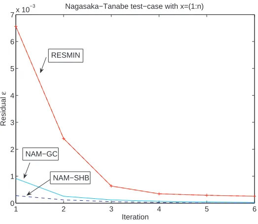
As we know that our algorithm will converge in a single iteration when x=u, we will not show the results of this test. Instead we will consider the case, where xi =i. The vector b in equation (1.1) can (of course) be obtained easily. Figure (1) shows the convergence speed of the most performing algorithms on this test case.
1 2 3 4 5 6
0 1 2 3 4 5 6 7x 10
−3 Nagasaka−Tanabe test−case with x=(1:n)
Iteration
Residual
ε
RESMIN
NAM−GC
NAM−SHB
Figure 1. Convergence Speed of some tested Algorithms in the Nagasaka case
As is well known Gauss’ algorithm is numerically unstable for such matrices. The RESMIN algorithm is however unable to reasonably approximate the solutionxbetter than 10−5. We have observed that the family of Kaczmarz algorithms (KACZ,KACZRT,KACSHB) has difficulties to properly estimate the last component ofx, despite of the small errorε. TheNA*M family of algorithms has a small errorεand reasonably estimates the last components ofx. For the NA*MRT algorithms, a good choice of the relaxation factorαallows us to reduce the number of iterations by a factor 2.
5.2.
Hilbert Matrix
1 2 3 4 5 6 0
0.05 0.1 0.15 0.2 0.25
Hilbert Test−case with x=(1:n)
Iteration
Residual
ε
GC
NAM−SHB
M−SHB M−GC
NAM−GC
Figure 2. Convergence Speed of some tested Algorithms in the Hilbert case
On figure (2) we observe the excellent behaviour of the conjugated gradient schemes, specifically adapted to this type of matrix. The NAMGC and MSHB however give solutions of comparable quality in only half of the number of iterations. We have finally observed a very slow convergence (speed) of the Richardson-Tanabe schemes (KACZRT, αNAMRT). Finally, MSHB converges faster than NAMSHB, but give a solution of comparable quality in the end.
5.3.
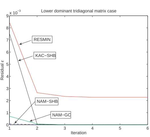
Lower diagonal dominant tri-diagonal Matrix
Our last test-case involves a tri-diagonal matrix of dimension 84, where the lower diagonal is dominant. Our matrixAis therefore the following matrix :
A=
1 1000 0
10000 1 . . . .
. 1 1000
0 10000 1
(5.15)
1 2 3 4 5 6 0
1 2 3 4 5 6 7 8 9x 10
−3 Lower dominant tridiagonal matrix case
Iteration
Residual
ε
RESMIN
KAC−SHB
NAM−GC NAM−SHB
Figure 3. Convergence Speed of some tested Algorithms in the tri-diagonal case
Except for theNA*M schemes, onlyRESMIN allows us to reasonably estimatexn, with only an approximation error of 8.6% (All other algorithms have a 90% error). However this algorithm offers only little precision ε. Except for MKAC, the NA*M algorithms give a solution with less than 2% approximation error for the last component ofx. It is clear that if we had used an upper-dominant matrix, the “edge”-effect would have been on the first component ofx, with similar results.
5.4.
Large Scale Systems
We prospect to test the proposed algorithms on several large scale systems. This section briefly mentions what three applications are thought about.
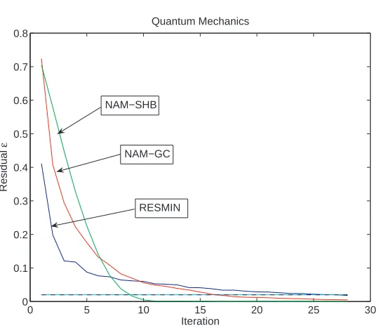
5.4.1. Three dimensional Schr¨odinger Equation
In [15, 16], the authors tackle the optical properties of self-assembled III-V and IV-IV nanostructures, in par-ticular for quantum information and telecommunication devices. The aim is to solve the strain-dependent Schr¨odinger equation in 8 band k.p theory.
0 5 10 15 20 25 30 0
0.1 0.2 0.3 0.4 0.5 0.6 0.7 0.8
Quantum Mechanics
Iteration
Residual
ε
RESMIN NAM−GC NAM−SHB
Figure 4. First results on a small Quantum mechanics test case
The horizontal line corresponds to the minimal requested accuracy. As we can observe, theNAMSHBalgorithms allows us to obtain required accuracy, in less iterations thanRESMIN. The former using matrix products, the latter only matrix-vector products. Work is in progress in order to formulate proposed numerical schemes using only products of matrices and vectors.
5.4.2. Unit Commitment
The Unit Commitment Problem (UCP) consists of defining the minimal-cost power generation schedule for a given set of power plants, thermal and hydraulic. We will focus on hydraulic valley management. The interconnected reservoirs and productions units, once modeled give way to a large linear system (from 5000 to 15000 variables).
We use Lagrangian relaxation, price decomposition and other optimization techniques to solve the UCP [6, 13], exploiting its highly decomposable structure. In this context, the sub-problem related to an hydraulic valley can be stated as a linear program.
The interior point method is currently used for solving this linear program (which is itself solved at each iteration of the price decomposition algorithm, typically 400 times). As is known, the linear system solved at each iteration of the interior point algorithm becomes more and more badly conditioned. The proposed algorithms might therefore improve the solution quality.
5.4.3. Electromagnetics
using eddy-current or geophysical exploration) the convergence of the classical iterative algorithms is far to be optimal (large number of iterations, slow convergence). The algorithms developed in this paper could be tested in such configurations and might be a way to greatly improve the speed/quality of some electromagnetic codes.
6.
Conclusions
Estimating efficiently the solution of an ill-conditioned linear system of equations is tricky.
The new approach we have developed, based on properties of stochastic matrices and lp norms, allows us to define in two steps algorithms for efficiently solving any ill-conditioned, and possibly singular, linear system of equations. First, we construct an approximation of a generalized inverse of the matrix of the system (which can be complex, rectangular and without specific structure). The second step consists in using this matrix in classical schemes as Richardson-Tanabe, Schultz-Hotelling-Bodewig or conjugate gradients. We also propose a generalization of the Kaczmarzs scheme, initially defined forl2 norm, as other possible scheme of resolution.
Even considering algorithms obtained with l1 norm, we reported outstanding performances (performance is understood as the capacity to retrieve as best as possible the exact solution). In this way, for any matrix A
or more specifically for positive semi-definite hermitian matrix, at least one of the proposed algorithms is more efficient than the algorithms we’ve tested. Hence :
• when A is regular, hermitian, positive-definite, we suggest to use the matrix R = ˆf(A) , in the pre-conditioned conjugate gradients scheme since, regarding the ill-conditioning snag, this scheme is more efficient and more robust than the classical conjugate gradients;
• for any matrixA, using the matrixR=αfnm(A∗)A∗fmn(A) in the Schultz-Hotelling-Bodewig’s scheme or in the conjugate gradients scheme gives very robust results regarding the ill-conditioning and error propagation.
For some ill-conditioned matrices with specific structure (tridiagonale, upper or lower dominance, . . . ), the proposed algorithms are able to correctly estimate some components of the solution-vector, whereas none of the known algorithms tested is able to do so.
When an existing algorithm is more efficient than those proposed (it is the case for the conjugate gradients with the Hilbert matrix test-case), one of proposed algorithms gives a solution with equivalent quality in approximatively two times less iterations.
Finally, regarding the first tests we have reported, it seems that the proposed algorithms are at least as efficient as the classical techniques tested. On our test-cases, they even seem to be more efficient. In addition, these algorithms are universal since they don’t need any restrictive hypothesis or conditions for application.
One can ask, when facing solving a pathological (huge, very ill-conditioned, specific structure, ...) linear system of equations, it would be possible to define low-cost procedures for extracting useful information of the solution without solving the system. For example the extreme values of the solution, the mean, the variance, etc. The promising approach of stochastic matrices developed here seems to be an interesting tool for exploring this way.
The authors would like to thank Sebastien Sauvage for providing us with data related to the Schr¨odinger equation application
References
[2] A. Bj¨orck and T. Elfving. Accelerated projection methods for computing pseudo-inverse solutions of a system of linear equations.
BIT, 19:145–163, 1979.
[3] E. Bodewig.Matrix Calculus. Interscience Ed., New York, 2 edition, 1959.
[4] Y. Censor. Row-action methods for huge and sparse systems and their applications.SIAM review, 23(4), 1981.
[5] G. Cimmino. Calcolo approssimato per le soluzioni dei sistemi dei equazioni lineari.Ricerca Sci. Progr. Tecn. Econom. Naz., 9:326–333, 1938.
[6] G. Cohen and D.L. Zhu. Decomposition-coordination methods in large-scale optimization problems. the non-differentiable case and the use of augmented langrangiens. 1, 1983.
[7] M.R. Hestenes and E. Stiefel. Methods of conjugate gradients for solving linear systems.Journal of Research of the National Bureau of Standards, 49(6):409–436, 1952.
[8] R.A. Horn and C.R. Johnson.Matrix analysis. Cambridge University Press, 1999.
[9] H. Hotelling. Further points on matrix calculations and simultaneous equations.Ann. Math. Statist., 14:440–441, 1943. [10] H. Hotelling. Some new methods in matrix calculation.Ann. Math. Statist., 14:1–34, 1943.
[11] S. Kaczmarz. Aufl¨osung von systemen linearer gleichlungen.Bulletin de l’Acad´emie Polonaise des Sciences et Lettres, A:355– 357, 1937.
[12] P. Lascaux and R. Theodor.Analyse num´erique matricielle appliqu´ee `a l’art de l’ing´enieur. Masson Editeur, Paris, 1987. [13] C. Lemar´echal and C. Sagasti´zabal. An approach to variable metric bundle methods.Lecture notes in Control and Information
Science, (197):144–162, 1994.
[14] H. Nagasaka. Error propagation in the solution of tridiagonal linear equations.Information Processing in Japan, 5:38–44, 1965. [15] S. Sauvage, P. Boucaud, F. Bras, G. Fishman, R.P.S.M. Lobo, F. Glotin, J.-M. Ort´ega, and J.-M. G´erard. Long polaron
lifetime in inas/gaas self-assembled quantum dots.Phys. Rev. Lett, (88):177–402, 2002.
[16] S. Sauvage, P. Boucaud, F. Bras, G. Fishman, R.P.S.M. Lobo, F. Glotin, R. Prazeres, J.-M. Ort´ega, and J.-M. G´erard. Polaron relaxation in inas/gaas self-assembled quantum dots.phys. stat. sol. (b), 238(2):254–257, 2003.
[17] G. Schultz. Iterative berechnung der reziproken matrix.Z. angew. Math. Mech., 13:57–59, 1933.
[18] K. Tanabe. Projection method for solving a singular system of linear equations and its applications.Numerische Mathematik, 17:203–214, 1971.